Glueball spectrum and the Pomeron in the Wilson loop approach

Abstract

Using a nonperturbative method based on asymptotic behaviour of Wilson loops we calculate masses of glueballs and corresponding Regge–trajectories. The only input is string tension fixed by meson Regge slope, while perturbative contributions to spin splittings are defined by standard $\alpha_{s}$ values. The masses of lowest glueball states are in a perfect agreement with lattice results. The leading glueball trajectory which is associated with Pomeron is discussed in details and its mixing with $f$ and $f^{\prime}$ trajectories is taken into account.

1 Introduction

The problem of existence of glueballs is one of the most interesting in QCD. Lattice calculations give definite predictions for a spectrum of such states [1-4], but experimental evidences are not conclusive [5,6]. Mixing between gluons and $q\bar{q}$-pairs makes a separation of glueballs a difficult problem. A theoretical study of glueballs in QCD started in [7-10] and is closely related to the problem of Pomeron – leading Regge pole, which determines the asymptotic behaviour of scattering amplitudes at very high energies. It is usually assumed that Pomeron in QCD is mostly gluonic object [11] and glueball resonances with vacuum quantum numbers and largest spins belong to this trajectory. Another interesting hypothetical Regge singularity is the ”odderon”, which has negative signature and $C$-parity and can be built out of at least 3 gluons. Most studies of the Pomeron and odderon singularities in QCD are based on applications of the perturbation theory [12].

In this paper we will address both the problem of spectra of glueballs and of the Pomeron (odderon) singularity using the method of Wilson-loop path integrals developed in papers [13-15]. The method is based on the assumption of the area law for Wilson loops at large distances in QCD, which is equivalent to the condition of confinement of quarks and gluons. It has been first applied to calculation of spectra of $q\bar{q}$–states in [16], baryons in [17] and glueballs in [18]. In this latter calculation rotation of the string between quarks or gluons was not taken into account, which lead to some distortion of mass spectra, notably the Regge slope was $1/8\sigma$ instead of string slope $1/2\pi\sigma$. In this paper we will use for glueballs more accurate calculational method developed in [14,15] for $q\bar{q}$–state, which yields the correct Regge slope (see [9] for numerical data and discussion). We also make a detailed study of possible corrections to large distance string dynamics due to small distance perturbative gluon exchanges (PGE) and will demonstrate that their influence on the mass spectrum of glueball states is rather small and can be computed as a correction. This is in contrast to the glueball spectrum in [8] where PGE in the form of the adjoint Coulomb potential was assumed as in many other papers on the subject. Instead we argue below in the paper, that PGE sums up to another series, the BFKL ladder [12], where loop corrections strongly suppress the final result , so that PGE can be disregarded in the first approximation. Our predictions for masses of lowest spin-averaged glueball states in units of $\sqrt{\sigma}$ are in a perfect agreement with results of recent lattice calculations [1-3]. In addition spin-orbit and spin-spin interactions are also calculated and found in a good agreement with lattice data.

The leading glueball Regge-trajectory is calculated in the positive $t$ region and is extrapolated to the scattering region of $t\leq 0$. The importance of mixing among this trajectory and $q\bar{q}$-trajectories ($f,f^{\prime}$) is emphasized; calculation of these mixing effects yields the leading Pomeron trajectory with $\alpha_{P}(0)>1$ $(\alpha_{P}(0)=1.1\div 1.2)$ in accord with experimental observations [20]. An interesting pattern of 3 colliding vacuum trajectories in the region $t>0$ is observed, which can be important for decay properties of resonances situated at these trajectories.

The paper is organized as follows. The field operators creating glueball states in general case and in the background field method are introduced in Section 2 and presented in Appendix 1. The general formalism of the Wilson loop path integrals and the resulting relativistic Hamiltonian is discussed in Section 2 and Appendix 2. The spectrum of spin-averaged glueball states following from this Hamiltonian is obtained in Section 2 and compared with corresponding lattice results. Spin splittings of glueball masses from both nonperturbative and perturbative parts are considered in Section 3 and Appendix 3 and 4. Resulting glueball spectrum is compared in the Section with lattice calculations. The influence of PGE on glueball masses and Regge - trajectories is discussed in Section 4. It is pointed out that effects of small-distances on glueball spectrum are small. Three–gluon glueballs are considered in Section 5. It is shown that the lowest 3g states have rather large mass $M_{3g}\approx 3.4GeV$. Relation between glueball Regge trajectories and the vacuum Pomeron trajectory is discussed in Section 6. In this Section and Appendix 5 effects of mixing between gluonic and $q\bar{q}$-Regge-trajectories are investigated.

Possible implications and improvements of the results of the paper are discussed in Conclusions.

2 General Formalism

Following [13,21], we separate gluonic fields $A_{\mu}$ into nonperturbative background $B_{\mu}$ and perturbative gluons $a_{\mu}$, $A_{\mu}=B_{\mu}+a_{\mu}$ , and consider two-gluon glueballs, described by the Green’s functions

$$G_{\mu\nu,\mu^{\prime}\nu^{\prime}}(x,y|x^{\prime},y^{\prime})=\langle\Psi^{(in)}(x,y)\Psi^{(out)}(x^{\prime},y^{\prime})\rangle_{a,B}=$$

$$\langle\Gamma^{(in)}G_{\mu\mu^{\prime}}(x,x^{\prime})G_{\nu\nu^{\prime}}(y,y^{\prime})\Gamma^{(out)}\rangle_{B}+{\rm perm}$$ (1)

where $\Psi^{(in)}(\Psi^{(out)})$ are glueball operators in the initial (final) state made of gluon field $a_{\mu}$ and $B_{\mu}$ (see Appendix 1 for explicit form of $\Psi^{(in),(out)}$ in lowest states); $G_{\mu\mu^{\prime}}$ is the gluon Green’s function of field $a_{\mu}$ in the background field $B_{\mu}$, namely

$$G_{\mu\nu}(x,y)=\langle x|(-\hat{D}^{2}\delta_{\mu\nu}-2ig\hat{F}_{\mu\nu})^{-1}|y\rangle_{B}$$ (2)

where $\hat{D}_{\mu}=\partial_{\mu}-ig\hat{B}_{\mu},~{}\hat{F}_{\mu\nu}$ is the field strength of the field $\hat{B}_{\mu}$ in the adjoint representation, and averaging over background $B_{\mu}$ is implied by angular brackets (where subscript $B$ will be omitted).

Referring the reader for details of derivation to refs. [13,18,21] and Appendix 2, one can write for (1) the path integral

$$G_{\mu\nu,\mu^{\prime}\nu^{\prime}}(x,y|x^{\prime},y^{\prime})=const\int^{\infty}_{0}ds\int^{\infty}_{0}ds^{\prime}DzDz^{\prime}e^{-K-K^{\prime}}\langle\Gamma^{(in)}W_{F}\Gamma^{(out)}\rangle$$ (3)

where $K=\frac{1}{4}\int^{s}_{0}(\frac{dz}{d\tau})^{2}d\tau,~{}~{}K^{\prime}$ is the same with primed $z,\tau,s$, and

$$\langle W_{F}\rangle=trP_{B}P_{F}\langle\exp\{ig\int_{C}B_{\mu}du_{\mu}+2ig\int^{s}_{0}\hat{F}d\tau+2ig\int^{s^{\prime}}_{0}\hat{F}d\tau^{\prime}\}\rangle$$ (4)

Here $P_{B},P_{F}$ are ordering operators of the color matrices $B_{\mu}$ and $\hat{F}$ respectively. As we shall see in section 3, the terms with $\hat{F}$ generate spin–dependent contribution of nonperturbative background, which is calculable and small, and we shall treat those terms perturbatively.

Neglecting $\hat{F}^{\prime}s$ as a first approximation and omitting for simplicity projection operators $\Gamma^{(in)},\Gamma^{(out)}$ which do not influence the form of resulting Hamiltonian, one arrives at the Wilson loop in the adjoint representation, for which one can use the minimal area law, confirmed by numerous lattice data [22] at least up to the distance of the order of $1fm$,

$$\langle W_{adj}\rangle=Z~{}exp(-\sigma_{adj}S_{min})$$ (5)

where we have included in $Z$ self-energy and nonasymptotic corrections, since (5) is valid for large loops with size $R,T\gg T_{g}$, where $T_{g}$ is the gluon correlation length.

Note, that we could treat (4) by the field correlator method [13,23], keeping only lowest (Gaussian) correlator $\langle F(x)F(y)\rangle$. In this case the leading term will again have the form (5); we shall use this method to evaluate contribution of the gluon spin terms $\hat{F}$ in (4); the result (5) is more general, since $\sigma_{adj}$ in (5) contains contribution of all correlators and is not connected to the Gaussian approximation.

Applying now the general method of [14] to the Green’s function (3), one introduces auxiliary (einbein) function $\mu(t)$ of the real time $t$ instead of the proper time $s,\tau$, via relation $d\tau=\frac{dt}{2\mu(t)}$, and einbein auxiliarly function $\nu(\beta,t)$ to get rid of the square root Nambu-Goto form for $S_{min}$ in (5). As a result one defines the hamiltonian $H$, through the equality $G\sim exp(-TH)$, where $T$ is the evolution parameter, taken here to be the center-of-mass time $T,0\leq t\leq T$.

The resulting relativistic Hamiltonian for two spinless gluons looks like [14]

$$H_{0}=\frac{p_{r}^{2}}{\mu(t)}+\mu(t)+\frac{L(L+1)}{r^{2}[\mu+2\int^{1}_{0}(\beta-\frac{1}{2})^{2}\nu d\beta]}+$$

$$+\int^{1}_{0}\frac{\sigma^{2}_{adj}d\beta}{2\nu(\beta,t)}r^{2}+\frac{1}{2}\int^{1}_{0}\nu(\beta,t)d\beta$$ (6)

Here $\mu(t)$ and $\nu(\beta,t)$ are positive auxiliary functions which are to be found from the extremum condition [14]. Their extremal values are equal to the effective gluon energy $\langle\mu\rangle$ and energy density of the adjoint string $\langle\nu\rangle$.

For the case $L=0$ the extremization over $\mu$ and $\nu$ yields a simple answer [14], coinciding with the Hamiltonian of the relativistic potential model

$$H_{0}=2\sqrt{p^{2}_{r}}+\sigma_{adj}r$$ (7)

An approximation made in [16-18] corresponds to the replacement of the operators $\mu(\tau),\nu(\tau,\beta)$ (which by extremization are expressed through operators $p,r$) by $c$ –numbers, to be found from extremization of eigenvalues of $H_{0}$. This yields another form, used in [18],

$$H^{\prime}_{0}=\frac{\mbox{\boldmath${\rm p}$}^{2}}{\mu_{0}}+\mu_{0}+\sigma_{adj}r$$ (8)

as can be seen from Table 3 of ref. [19], eigenvalues of (8) are about 5% higher than those of $H_{0}$. The value of $\sigma_{adj}$ in (8) can be found from the string tension of $q\bar{q}$ system, since the Casimir scaling found on the lattice [22] predicts that

$$\sigma_{adj}=\frac{C_{2}(adj)}{C_{2}(fund)}\sigma_{fund}=\frac{9}{4}\sigma_{fund}$$ (9)

For light quarks the value of $\sigma_{fund}$ is found from the slope of meson Regge trajectories and is equal to

$$\sigma_{fund}=\frac{1}{2\pi\alpha^{\prime}}\approx 0.18GeV^{2}$$ (10)

¿From that we find

$$\sigma_{adj}\approx 0.40GeV^{2}$$ (11)

In what follows the parameter $\mu$ and its optimal value $\mu_{0}$, which enters in (8) play very important role. The way they enter spin corrections in Section 3 and magnetic moments shows that $\mu_{0}$ plays the role of effective (constituent) gluon mass (or constituent quark mass in the equation for the $q\bar{q}$ system).

In contrast to the potential models, where the constituent mass of gluons and quarks is introduced as the fixed input parameter in addition to the parameters of the potential, in our approach $\mu_{0}$ is calculated from the extremum of the eigenvalue of equation (8), which yields

$$\mu_{0}(n)=\sqrt{\sigma}(\frac{a(n)}{3})^{3/4},M_{0}(n)=4\mu_{0}(n)$$

where $\sigma=\sigma_{adj}$ for gluons and $\sigma=\sigma_{f}$ for massless quarks, and a(n) is the eigenvalue of the reduced equation $\frac{d^{2}\psi}{d\rho^{2}}+(a(n)-\rho-L(L+1)/\rho^{2})\psi=0$. The first several values of $a(n)$ and $\mu_{0}(n)$ are given in the Table 1, and will be used in Section 3.

Note that our lowest ”constituent gluon mass” $\mu_{0}(n=L=0)=0.528GeV$ (for $\sigma_{f}=0.18GeV)$ is not far from the values introduced in the potential models, the drastic difference is that $\mu_{0}$ depends on $n,L$ and grows for higher states, and is calculable in our case.

The eigenvalues of $H_{0}$, Eq. (7), for $L=0$ and different $n=0,1,2,...$ are given in Table 2 for $\sigma_{adj}=\frac{9}{4}\sigma_{fund}=\frac{9}{4}0.18GeV^{2}$. The mass spectrum for $L>0$ is given by eigenvalues of $H_{0}$, Eq.(6), and was studied in [14]. With the 5% accuracy of WKB approximation one can exploit much simpler expressions found in [19], which predict for $L>0$ the eigenvalues shown in Table 3. An independent numerical estimation of the rotating string spectrum was done in [24] and yields similar eigenvalues.

¿From Tables 1,2,3 and [24] one can see that mass spectra of the Hamiltonian (6) are described with a good accuracy by a very simple formula

$$\frac{M^{2}}{2\pi\sigma}=L+2n_{r}+c_{1}$$ (12)

where $L$ is the orbital momentum, $n_{r}$ –radial quantum number and $c_{1}$ is a constant $\approx 1.55$. It describes an infinite set of linear Regge-trajectories shifted by $2n_{r}$ from the leading one ($n_{r}=0)$. The only difference between light quarks and gluons at this stage is the value of $\sigma$, which determines the mass scale.

Thus the lowest glueball state with $L=0,n_{r}=0$ according to Table 2 and eq. (12) has $M^{2}=4.04GeV^{2}.$

It corresponds to a degenerate $0^{++}$ and $2^{++}$ state.

$$M=2.01GeV$$ (13)

In order to compare our results with the corresponding lattice calculations [1-4 ] it is convenient to consider the quantity $\bar{M}/\sqrt{\sigma_{f}}$, which is not sensitive to the choice of string tension $\sigma$  .

¿From these data we have for $L=0,n_{r}=0$ states the spin averaged mass

$$\frac{\bar{M}}{\sqrt{\sigma_{f}}}=\frac{M(0^{++})+2M(2^{++})}{3}\frac{1}{\sqrt{\sigma_{f}}}$$ (14)

the value $4.61\pm 0.1$, which should be compared to our prediction $\bar{M}^{theor}(L=0,n_{r}=0)/\sqrt{\sigma_{f}}=4.68.$

For radially excited state our theory predicts

$$\frac{\bar{M}^{theor}}{\sqrt{\sigma_{f}}}(L=0,n_{r}=1)=7.0$$ (15)

Lattice data [1] give for this quantity

$$\frac{\bar{M}^{lat}}{\sqrt{\sigma_{f}}}(L=0,n_{r}=1)=6.56\pm 0.55$$ (16)

For $L=1,S=1$ states one can define spin-averaged mass in a similar way

$$\frac{\bar{M}}{\sqrt{\sigma_{f}}}=\frac{M(0^{-+})+2M(2^{-+})}{3}\frac{1}{\sqrt{\sigma_{f}}}$$ (17)

lattice data [1-4] yield

$$\frac{\bar{M}^{lat}}{\sqrt{\sigma_{f}}}(L=1,n_{r}=0)=6.11\pm 0.38$$ (18)

which is in a reasonable agreement with our prediction

$$\frac{\bar{M}^{theor}}{\sqrt{\sigma_{f}}}(L=1,n_{r}=0)=6.0.$$ (19)

For $L=2,n_{r}=0$ and $L=1,n_{r}=1$ we have the spin averaged state we have

$$\frac{\bar{M}^{theor}(l=2,n_{r}=0)}{\sqrt{\sigma_{f}}}=7.0;\frac{\bar{M}^{theor}}{\sqrt{\sigma_{f}}}(L=1,n_{r}=1)=8.0$$ (20)

Lattice data [1] yield respectively $7.7\pm 0.4$ and $7.94\pm 0.48$. Note that in the first multiplet lattice data exist only for $3^{++}$. The overall comparison of spin-averaged masses computed by us and on the lattice is shown in Table 4.

Thus we come to the conclusion that the spin–averaged masses obtained from purely confining force with relativistic kinematics for valence gluons are in a good correspondence with lattice data, which implies that PGE shifts of glueball masses in lattice calculations is small.

3 Spin splittings of glueball masses

Here we shall treat spin effects in a perturbative way; a glance at our predictions in Table 5 and at the lattice results given in Table 6 tells that spin splittings in glueball states apart from $2^{++}-0^{++}$ amount to less than 10-15% of the total mass, and hence perturbative treatment is justified to this accuracy level.

Before starting actual calculations of spin splittings one should choose between two possible strategies (and corresponding physical mechanisms) of treating gluon polarizations. In the first approach one insists on the transversality condition and on the resulting two gluon polarizations as for the free gluon [7], (this is the procedure accepted e.g. in [28]).

In the second approach it is assumed that gluon has acquired nonzero mass due to the adjacent string, similarly to the case of $W^{\pm},Z^{0}$, where mass is created by the Higgs condensate. In this case one has 3 massive gluon polarizations and the spin coupling scheme of two gluons can be taken as the $LS$ scheme with the characteristic $J^{PC}$ pattern of lowest levels, which is observed in lattice calculations [1-4].

Therefore we choose the second approach and consider gluon spin operator $\mbox{\boldmath${\rm S}$}^{(i)},i=1,2$, total spin operator $\mbox{\boldmath${\rm S}$}=\mbox{\boldmath${\rm S}$}^{(1)}+\mbox{\boldmath${\rm S}$}^{(2)}$ and orbital angular momentum ${\rm L}$, the total angular momentum ${\bf J}={\bf L}+{\bf S}$, and assign to each level (mass) not only conserved values of $J^{PC}$, but also values of $L,S$ (which in some cases may have admixture of $L^{\prime}=L\pm 2$, $S^{\prime}=S\pm 2$, but this admixture in general case is small).

The detailed discussion of the gluon mass generation in the context of gauge invariance and symmetry breaking (as also in the electroweak case) is relegated to a separate publication.

The two–gluon mass operator can be written as

$$M=M_{0}(n,L)+\mbox{\boldmath${\rm S}$}\mbox{\boldmath${\rm L}$}M_{SL}+\mbox{\boldmath${\rm S}$}^{(1)}\mbox{\boldmath${\rm S}$}^{(2)}M_{SS}+M_{T},$$ (21)

where $M_{0}$ is the eigenvalue of the Hamiltonian $H\equiv H_{0}+\Delta H_{pert}$, and $H_{0}$ is given in (7) (or its approximation in (8)), while $\Delta H_{pert}$ is due to perturbative gluon exchanges and discussed in the next section.

To obtain three other terms in (21) one should consider averaging of the operators $\hat{F}$ in the exponent of (4) and take into account that

$$-2i\hat{F}_{\mu\nu}=2(\mbox{\boldmath${\rm S}$}^{(1)}\mbox{\boldmath${\rm B}$}^{(1)}+\tilde{\mbox{\boldmath${\rm S}$}}^{(1)}\mbox{\boldmath${\rm E}$}^{(1)})_{\mu\nu}$$ (22)

and similarly for the term in the integral $\int\hat{F}d\tau^{\prime}$, with the replacement of indices $1\to 2$. Here gluon spin operators are introduced, e.g.

$$(S^{(1)}_{m})_{ik}=-ie_{mik},~{}~{}i,k=1,2,3,(\tilde{S}^{(1)}_{m})_{i4}=-i\delta_{im}$$ (23)

Two remarks are in order here: i) the gluon spin enters via the integral $\int 2{\bf SB}d\tau^{\prime}=\int\frac{{\bf SB}}{\mu(t)}dt$, where $\mu(t)$ with its extremum value $\mu_{0}$ is the same as in (6), (8) (for details see Appendix 2). ii) the main part of the Hamiltonian, $H_{0}$ is diagonal in spin indices $i,k$; while the spin–dependent part (22) is treated as a perturbation, hence the admixture of the 4-th polarization due to $\tilde{S}$ in (23) does not appear to the lowest order.

The detailed derivation of spin–dependent terms is done in the Appendix 3, here we only quote the results. Since the structure of the term $\hat{F}$ in (4) due to (22) is the same as in case of heavy quark with the replacement of the heavy quark mass by the effective gluon parameter $\mu_{0}$ (see (8)), one can use the spin analysis of a heavy quarkonia done in [25], to represent the spin–dependent part of the Hamiltonian in the form similar to that of Eichten and Feinberg [26]

$$\Delta H_{s}=\frac{\mbox{\boldmath${\rm S}$}\mbox{\boldmath${\rm L}$}}{\mu^{2}_{0}}(\frac{1}{r}\frac{dV_{1}}{dr}+\frac{1}{r}\frac{dV_{2}}{dr})+\frac{\mbox{\boldmath${\rm S}$}^{(1)}\mbox{\boldmath${\rm S}$}^{(2)}}{3\mu^{2}_{0}}V_{4}(r)+$$

$$+\frac{1}{3\mu_{0}^{2}}(3(\mbox{\boldmath${\rm S}$}^{(1)}\mbox{\boldmath${\rm n}$})(\mbox{\boldmath${\rm S}$}^{(2)}\mbox{\boldmath${\rm n}$})-\mbox{\boldmath${\rm S}$}^{(1)}\mbox{\boldmath${\rm S}$}^{(2)})V_{3}(r)+\Delta V$$ (24)

where $\Delta V$ contains higher cumulant contributions which can be estimated to be of the order of 10% of the main term in (24) and will be neglected in what follows. Note that spin of gluon is twice that of quark, therefore spin–orbit and spin–spin terms for glueballs are effectively twice and four times larger respectively than for the quarkonia case.

The functions $V_{i}(r)$ are the same as for heavy quarkonia [25] except that Casimir operators make them $9/4$ times larger; the corresponding expressions of $V_{i}(r)$ in terms of correlators $D(x),D_{1}(x)$ [23], are given in the Appendix 3. Both $D$ and $D_{1}$ are measured on the lattice [27] and $D_{1}$ is found to be much smaller than $D$. Therefore one can neglect the nonperturbative part of $V_{3}(r)$, while that of $V_{4}$ turns out to be also small numerically, $M_{SS}(nonpert.)<30MeV$, and we shall also neglect it.

The only sizable spin–dependent nonperturbative contribution comes from the term $\frac{dV_{1}}{dr}$ (Thomas precession) and can be written at large distances as

$$\Delta H(Thomas)=-\frac{\sigma_{adj}}{r}\frac{\mbox{\boldmath${\rm L}$}\mbox{\boldmath${\rm S}$}}{2\mu^{2}_{0}}$$ (25)

Now we come to the point of perturbative contributions to spin splittings. The simplest way to calculate those to the order $O(\alpha_{s})$ (and this procedure holds true for quarkonia) is to represent perturbative gluon exchanges by the same Eichten–Feinberg formulas (24) where one should keep in $V_{i}(r)$ only perturbative contributions to correlators $D$ and $D_{1}$ in (A3.8)-(A3.11); then to the order $O(\alpha_{s})$ one obtains

$$\frac{1}{r}\frac{dV_{1}^{(pert)}}{dr}=0,~{}~{}\frac{dV_{2}^{(pert)}}{dr}=\frac{C_{2}(adj)\alpha_{s}}{r^{2}},$$ (26)

$$V_{3}^{(pert)}=\frac{3C_{2}(adj)\alpha_{s}}{r^{3}},$$ (27)

$$V_{4}^{(pert)}=8\pi C_{2}(adj)\alpha_{s}\delta^{(3)}(r)$$ (28)

However this procedure should be corrected for glueballs since $i)$ valence and exchanged gluons are identical and $ii)$ there is a 4–gluon vertex in addition. The corresponding calculations have been done in [28], which show that corrections amount to the multiplication in (26) with the factor $3/4$ and in (28) with the factor $5/8$.

With the account of these corrections the corresponding matrix elements in (21) look like

$$M_{SL}^{(pert)}=\frac{3C_{2}(adj)}{4\mu_{0}^{2}}\langle\frac{\alpha_{s}}{r^{3}}\rangle$$ (29)

$$M_{SS}^{(pert)}=\frac{5\pi C_{2}(adj)}{3\mu_{0}^{2}}\langle\alpha_{s}\delta^{(3)}(r)\rangle$$ (30)

$$M_{T}^{(pert)}=\frac{C_{2}(adj)}{\mu_{0}^{2}}\langle\frac{\alpha_{s}}{r^{3}}(3\mbox{\boldmath${\rm S}$}^{(1)}\mbox{\boldmath${\rm n}$}\mbox{\boldmath${\rm S}$}^{(2)}\mbox{\boldmath${\rm n}$}-\mbox{\boldmath${\rm S}$}^{(1)}\mbox{\boldmath${\rm S}$}^{(2)})\rangle$$ (31)

¿From (30) one can see that $M_{SS}$ can be written as

$$M_{SS}=\frac{5\alpha_{s}}{4\mu^{2}_{0}}|R(0)|^{2}$$ (32)

To make simple estimates, we shall neglect first the interaction due to PGE between valent gluons. Indeed we show in the next section that this interaction cannot be written as Coulomb potential between adjoint charges, and comparison to perturbative BFKL Pomeron theory [12] shows that it is much weaker than Coulomb potential. Neglecting this interaction altogether, one gets the lower bound of spin-dependent effects, since all matrix clements, like $\langle\delta^{(3)}(r)\rangle,\langle\frac{1}{r}\rangle,\langle\frac{1}{r^{3}}\rangle$ are enhanced by attractive Coulomb interaction.

For purely linear potential one has simple relation, not depending on radial quantum number $n$ [29]

$$|\Psi(0)|^{2}=\frac{|R(0)|^{2}}{4\pi}=\frac{\mu_{0}\langle V^{\prime}(r)\rangle}{4\pi}=\frac{\mu_{0}\sigma_{adj}}{4\pi}$$ (33)

Using (33) and $M_{0}=4\mu_{0}$, and taking $M_{0}$ from Table 1, one obtains

$$M_{SS}=\frac{5\alpha_{s}\sigma_{adj}}{M_{0}},$$ (34)

and for $n_{r}=0,1$ and $\alpha_{s}=0.3$ the spin-spin splitting is

$$M_{SS}(n_{r}=0)=0.3GeV,M_{ss}(n_{r}=1)=0.20GeV$$ (35)

For $M(0^{++})$ and $M(2^{++})$ one has the values given in Table 5 for $\sigma_{f}=0.18GeV^{2}$ and for the sake of comparison with lattice calculations in Table 6 for $\sigma_{f}=0.228GeV^{2}$ and $\alpha_{s}=0.3$.

For $L>0$ one needs to compute spin corrections $M_{SL}$ and $M_{T}$. First of all one can simplify matter using the equation (it is derived in the same way, as (33) was derived in [29], for details see Appendix 4))

$$L(L+1)\langle\frac{1}{r^{3}}\rangle=\frac{\mu_{0}}{2}\langle V^{\prime}(r)\rangle$$ (36)

For $V(r)=\sigma_{adj}r$ both $M_{SL}^{(pert)}$ and $M_{T}^{(pert)}$ are easily calculated and listed in Table 7.

The nonperturbative part of spin splittings is due to the Thomas term, ($\frac{dV_{1}}{dr}+\frac{dV_{2}}{dr}$), and is calculated numerically using the exponential form of $D,D_{1}$ found on the lattice [27], for details see [25].

The resulting figures for $\triangle M_{Thomas}$ are given in Table 7. Combining all corrections and values of $M_{0}$ from Table 2,3 one obtains glueball masses shown in Table 5 for $\sigma_{f}=0.18GeV^{2}$ and compared with lattice data in Table 6 for $\sigma_{f}=0.228GeV^{2}$.

One can see in Table 6 that calculated spin splittings of lowest levels are in good agreement with lattice data. This is another phenomenological manifestation of the PGE suppression in the glueball system; indeed had we taken PGE in the adjoint Coulomb form with $\alpha_{s}=0.3$, we would obtain 3 times larger spin splittings [18].

The general feature of spin–dependent contribution $\Delta H_{s}$ is that it dies out very fast with the growing orbital or radial number, which can be seen in the appearance of the $\mu^{2}_{0}$ factor in the denominator of (29-31).

Indeed, from (8) one can derive that $M_{0}\approx 4\mu_{0}$ and therefore $\Delta H_{s}\sim\frac{1}{M^{2}(n,L)}\langle O(\frac{1}{r})\rangle$, where $O$ stands for terms like $const.\frac{1}{r}$ or $const^{\prime}.\frac{1}{r^{3}}$ (from perturbation theory). Hence spin splittings of the radial recurrence of states $0^{++},2^{++}$ or $0^{-+},2^{-+}$ should be smaller than the corresponding ground states. This feature is also well supported by the lattice data in Table 5.

4 Perturbative gluon ladders and glueballs

In many analytic calculations of glueball masses it is postulated that there is a Coulomb-type interaction between valence gluons, which differs from the $q\bar{q}$ case by the Casimir factor, $C_{2}(adj)=3$ instead of $C_{2}(fund)=\frac{4}{3}$. Before going into the details of the question how the perturbative gluon exchanges give rise to the Coulomb kernel, we here first assume that this is indeed the case, and correspondingly calculate the eigenvalues of the hamiltonian

$$H=H^{\prime}_{0}-\frac{C_{2}(adj)\alpha_{s}}{r}$$ (37)

where $H^{\prime}_{0}$ is given in (8). The resulting masses are listed in Table 8 (the first three lines) for $\alpha_{s}=0,0.2,0.3,0.39$.

One can see a drastic decrease of the mass due to the Coulomb attraction, especially for L=0. For a conservative value $\alpha_{s}=0.3$ this mass drops down by 0.5 GeV.

This is much larger than in the $q\bar{q}$ case [13,19], evidently due to the large Casimir factor.

Another characteristics of the Coulomb shift, which is useful for the comparison with perturbative Pomeron approach [12], is the Regge slope $\alpha^{\prime}_{G}(0)$ and Regge intercept $\alpha_{G}(0)$ of the glueball trajectory drawn as a straight line through the glueballs with $L=0(2^{++})$ and $L=0(4^{++})$ . These values are given in the last two lines of Table 8, and show a drastic increase of the intercept due to Coulomb interaction by $\Delta\alpha_{G}(0)\approx 0.64$ for $\alpha_{s}=0.3$.

This will be compared later in this chapter with a similar large shift of the perturbative Pomeron trajectory $\Delta\alpha_{P}(0)$ in the lowest $O(\alpha_{s})$ approximation [12] and with much smaller value of $\Delta\alpha_{P}(0)$ in the next (one–loop) approximation [30].

This comparison casts one more doubt on the validity of the assumption about the presence of the adjoint Coulomb interaction in the form (37).

A similar conclusion can be deduced from spin-averaged eigenvalues. Indeed for the Hamiltonian

$$H=H^{\prime}_{0}-\frac{C_{2}(adj)\alpha_{s}}{r}$$ (38)

the eigenvalues are given in Table 8.

One can see that for $L=0$ both $\alpha_{s}=0.3$ and $0.39$ strongly contradict data, which shows that perturbative gluon ladder strongly differs from the adjoint Coulomb interaction, moreover the overall agreement of our results for $M_{0}$ (where no Coulomb interaction is present) with spin averaged lattice masses tells that PGE is strongly reduced on the lattice.

To study this point in detail one should consider the set of perturbative gluon exchanges and compare them to the BFKL diagrams describing the perturbative Pomeron [12].

First of all one should look into the mechanism which produces color Coulomb interaction, and it is instructive to compare quark-antiquark and gluon - gluon system from this point of view. For both systems there are diagrams of gluon exchanges in the order $O(g^{2})$, and in addition for gluon - gluon system there is in the same order the diagram of contact interaction, which affects the hyperfine splitting [28].

The main point is whether and how these diagrams are summed up to produce the color Coulomb kernel in the exponent, entering the Green’s function of the system. For the $q\bar{q}$ system (neglecting spin degrees of freedom for simplicity of comparison) one has the exact Feynman-Schwinger representation

$$G_{q\bar{q}}=\int dsd\bar{s}DzD{\bar{z}}e^{-K-\bar{K}}\langle W(C_{z\bar{z}})\rangle$$ (39)

where the Wilson loop is along the paths $z,\bar{z}$ integrated in (39). One can use the cluster expansion for purely perturbative gluons in $W(C)$ as was done e.g. in [13,21]

$$\langle W(C)\rangle=exp[-C_{2}\frac{g^{2}}{2}\int\limits_{c}\int\limits_{c}\frac{dz_{\mu}d\bar{z}_{\mu}}{(z-\bar{z})^{2}}+0(g^{4})]$$ (40)

For straight-line trajectories $z(\tau),\bar{z}(\tau^{\prime})$ (e.g. for static quarks) the integral in the exponent of (41) readily yields the color Coulomb potential, $\langle W\rangle\sim exp(\frac{C_{2}\alpha_{s}}{r}t)$.

For light quarks one can consider the integral in the exponent of (40) as the full-fledged relativistic Coulomb kernel. It is legitimate to keep this kernel which is $O(g^{2})$ in the exponent,neglecting $O(g^{4})$ additional terms provided the Coulomb kernel yields some amplification.

This is indeed true in the nonrelativistic region (where Coulomb correction are of the order $\frac{\alpha_{s}}{u},u\ll 1$) or at small distances (high energies) where this kernel yields double logarithmic terms [31]. Let us turn now to the $gg$ system (the same is true a fortiori for the three-gluon system).

In (3) we have derived the $gg$ Green’s function for valent perturbative gluons in the nonperturbative background. The similarity of forms (3) and (39) is only superficial, since the Wilson loop in (39) contains both perturbative and nonperturbative contributions and one may argue, that perturbative exchanges dominate at small distances, and hence exponentiate as in (40) and consequently give forth the color Coulomb kernel.

In contrast to that , in (3) $\langle W_{F}\rangle$ contains only nonperturbative fields $B_{\mu}$, yielding confining string between gluons, but no perturbative exchanges at all. In the framework of the background perturbation theory the perturbative vertices $0(a^{3})$ and $0(a^{4})$ enter the interaction Lagrangian, and there is a priori no guarantee that gluon exchanges produced by these vertices exponentiate to give a color Coulomb kernel. (Note that there is a difference between gluon exchanges, and spin - dependent vertices considered in the previous chapter, since the latter are taken as a perturbation in the lowest order, and there is no need for them to exponentiate to the Coulomb ladder).

Having all this in mind, we turn our attention to the subset of graphs which is summed up in the BFKL approach [12], and which is distinguished by the principle of leading diagrams in the high–energy scattering, or in another setting, by the summation of ladders for the leading Regge trajectory in the $t$–channel. Since these ladders are dominant perturbative series (see [12]) for the Pomeron trajectory, we can consider the same contribution in our circumstances - for calculation of glueball masses, extending in this way BFKL – type analysis from Pomeron–generating glueballs ($4^{++},2^{++}etc$) to all others, and having in mind, that this may give only an estimate of the order of magnitude.

Thus our purpose is now to estimate the contribution of the BFKL diagrams to the glueball masses (perturbative mass shift) and compare it to the usual color Coulomb contribution.

In order to estimate effects of small distance contributions we shall use the analysis of these effects on gluonic Regge–trajectories not from the glueballs mass spectra at positive $t$, but for $t=0$. Extensive calculations of the gluonic Pomeron trajectory intercept have been carried out in the leading log approximation (LLA) [12] and $\alpha_{s}$ corrections were calculated recently [30]. It has been shown that the leading Regge singularity corresponds to a sum of ladder type diagrams, where exchanged gluons are reggeized. In the leading approximation an intercept of this singularity is equal to [12]

$$\alpha_{P}(0)=1+\alpha_{s}\frac{4N_{c}}{\pi}ln2$$ (41)

The shift from the noninteracting gluons point $\alpha_{P}(0)=1$ is equal to $\Delta=\alpha_{P}(0)-1\approx 0.5$ for $\alpha_{s}\approx 0.2$. This rather large shift is strongly reduced by $\alpha_{s}$ corrections [30]

$$\Delta=\alpha_{s}\frac{12}{\pi}ln2(1-C\alpha_{s})$$ (42)

The coefficient $C$ is rather large $(\approx 6.5)$ and the $\alpha_{s}$ correction strongly reduces $\Delta$. Its value depends on the renormalization scheme and scale for $\alpha_{s}$. In the ”physical” (BLM) scheme values of $\Delta$ are in the region $0.15\div 0.17$ [30]. In this approximation the leading gluonic singularity is Regge-pole. and we can estimate mass-shift of the lowest glueball state using this result and assuming that the slope $\alpha^{\prime}_{P}=\frac{1}{2\pi\sigma_{adj}}\approx 0.4GeV^{-2}(11)$ will not be strongly modified by perturbative effects. Thus one can expect that characteristic shift due to perturbative effects in $\bar{M}^{2}(L=0,n_{r}=0),\delta\bar{M}^{2}\approx\Delta/\alpha^{\prime}_{adj}\approx(0.38\div 0.48)GeV^{2}$. This corresponds to the shift in $\bar{M}(L=0,n_{r}=0),\delta\bar{M}\approx\delta\bar{M}^{2}/2\bar{M}\approx 0.1GeV$. This shift should be compared with much larger mass shift from pure Coulomb interaction given in Table 8. Thus the $O(\alpha_{s})$ correction to the BFKL ladder gives a strong suppression of PGE series and may be a possible explanation why Coulomb –like attraction is not seen neither in spin–averaged masses $\bar{M}(L,n_{r})$, nor in spin splittings. It should be noted that this is only a rough estimate of the perturbative effects because higher orders of the perturbation theory can modify this result.

5 Three–gluon glueballs

The three–gluon system can be considered in the same way, as it was done for the two-gluon glueballs. The $3g$ Green’s function $G^{(3g)}$ is obtained as the background–averaged product of 3 one–gluon Green’s function, in full analogy with (1). Assuming large $N_{c}$ limit for simplicity and neglecting spin splittings and projection operators one arrives at the path integral (cf equation (3))

$$G^{(3g)}=const\prod^{3}_{i=1}\int^{\infty}_{0}ds_{i}Dz^{(i)}e^{-K_{i}-\sigma S_{i}}$$ (43)

where $\sigma\equiv\sigma_{fund}$, since every gluon is connected by a fundamental string with each of his neighbors.

Using as before the method of [13,14] and three–body treatment of [17] one obtains omitting spin–dependent terms the following Hamiltonian (we assume symmetric solution with equal $\mu_{i}(\tau)\equiv\mu(\tau),i=1,2,3$ (no orbital excitations was assumed as in (8))

$$H^{(3g)}=\frac{\mbox{\boldmath${\rm p}$}^{2}_{\eta}+\mbox{\boldmath${\rm p}$}^{2}_{\xi}}{2\mu}+\frac{3\mu}{2}+\sigma\sum^{3}_{i<j=1}r_{ij}$$ (44)

Here $r_{ij}=|\mbox{\boldmath${\rm r}$}_{i}-\mbox{\boldmath${\rm r}$}_{j}|$, and $\mbox{\boldmath${\rm r}$}_{i}$ is the space coordinate of the i-th gluon, while $\mbox{\boldmath${\rm\xi}$},\mbox{\boldmath${\rm p}$}_{x}i$ and $\mbox{\boldmath${\rm\eta}$},\mbox{\boldmath${\rm p}$}_{\eta}$ are defined as

$$\mbox{\boldmath${\rm\eta}$}=\frac{\mbox{\boldmath${\rm r}$}_{1}-\mbox{\boldmath${\rm r}$}_{2}}{\sqrt{2}},~{}~{}\mbox{\boldmath${\rm\xi}$}=\sqrt{\frac{3}{2}}(\frac{\mbox{\boldmath${\rm r}$}_{1}+\mbox{\boldmath${\rm r}$}_{2}}{2}-\mbox{\boldmath${\rm r}$}_{3}),~{}~{}\mbox{\boldmath${\rm p}$}_{\xi}=\frac{1}{i}\frac{\partial}{\partial_{\mbox{\boldmath${\rm\xi}$}}},~{}~{}\mbox{\boldmath${\rm p}$}_{\eta}=\frac{1}{i}\frac{\partial}{\partial_{\mbox{\boldmath${\rm\eta}$}}}$$ (45)

To simplify treatment further, we shall consider $\mu$ as a constant to be found from the extremum of eigenvalues, as in (8), which in that case provided some 5% increase in eigenvalues (see Table 3 of [19]), and what we expect also in this case.

To find eigenvalues of $H^{(3g)}$ one can use the hyperspherical method introduced in [32] and applied to the $3q$ system in [17]. Defining hyperradius $\rho$, $\rho^{2}=\mbox{\boldmath${\rm\eta}$}^{2}+\mbox{\boldmath${\rm\xi}$}^{2}$, one obtains one–dimensional equation for the eigenfunction $\chi^{K}_{n}(\rho)\equiv\chi(\rho)$,($K$ is the grand angular momentum $K=0,1,2...$, and $n$ –radial quantum number).

$$-\frac{1}{2\mu}\chi^{\prime\prime}+U_{eff}(\rho)\chi(\rho)=M\chi(\rho)$$ (46)

where

$$U_{eff}(\rho)=\frac{1}{2\mu\rho^{2}}(K^{2}+4K+\frac{15}{4})+\frac{32\sqrt{2}}{5\pi}\rho\sigma$$ (47)

Solution of (46) is expressed through generalized Airy functions.

A reliable (within few percent of accuracy) estimate of $M$ is obtained when one replaces $U_{eff}(\rho)$ by the oscillator well, with the center at the minimum of $U_{eff}(\rho),~{}~{}\rho=\rho_{0}$, and frequency $\omega_{0}$ expressed through $U^{\prime\prime}_{eff}(\rho_{0})$. For $K=0$ one has

$$\rho_{0}=(\frac{75\pi}{128\sqrt{2}\mu\sigma})^{1/3},~{}~{}\omega_{0}=(\frac{45}{4\mu^{2}\rho^{4}_{0}})^{1/2}$$ (48)

In this way one obtains

$$M(\mu)=\frac{3\mu}{2}+36(\frac{\sigma^{2}}{45\mu\pi^{2}})^{1/3}+\frac{\omega_{0}}{2}$$ (49)

and minimization of $M(\mu)$ in $\mu$ yields

$$\mu_{0}\cong(1.6)^{1/4}(\frac{8\sigma}{3\pi})^{1/2};~{}~{}M(\mu_{0})=6\mu_{0}+\frac{\omega_{0}}{2}=6\mu_{0}+(\frac{8}{5})^{3/4}(\frac{3\sigma}{\pi})^{1/2}$$ (50)

For $\sigma=0.18GeV^{2}$ one obtains $\omega_{0}=1.18GeV$ and $\mu_{0}=0.44GeV$, hence the minimal eigenvalue is

$$M_{0}=3.23GeV$$ (51)

This spin–averaged value is listed in Table 4. Radial excitations are given by an approximate equation

$$M_{n}=6\mu_{0}+\frac{\omega_{0}}{2}+n\omega_{0},~{}~{}n=0,1,2...$$ (52)

Orbital excitations yield increase in mass of the order

$$\Delta M^{K}\sim\frac{K^{2}+4K}{2\mu\rho^{2}_{0}},$$ (53)

which for lowest excitation gives

$$\Delta M^{K=1}\sim 1GeV$$ (54)

almost the same amount, as for the radial excitation.

Coulomb shift (if Coulomb interaction existed between gluons), would be enormous: $\Delta M(Coulomb)=-1.3GeV$. However here one can use the same arguments as for two–gluon glueballs and drop the color Coulomb interaction between gluons altogether.

Finally we turn to the question of quantum numbers and spin splittings of the $3g$ states.

According to (27), perturbative hyperfine interaction is given by matrix elements

$$\Delta M_{SS}=\sum_{i>j}\langle\mbox{\boldmath${\rm S}$}^{(i)}\mbox{\boldmath${\rm S}$}^{(j)}\frac{5\pi C_{2}(fund)}{3\mu_{0}^{2}}\alpha_{s}\delta^{(3)}(\mbox{\boldmath${\rm r}$}_{ij})\rangle$$ (55)

Note that in the large $N_{c}$ limit gluon lines are replaced by double fundamental lines and planar gluon exchanges occur with fundamental charge, hence the fundamental Casimir operator in (55).

For the $K=0$ state the wave function depends only on hyperradius $\rho$ and one has

$$\langle\delta^{(3)}(\mbox{\boldmath${\rm r}$}_{ij})\rangle=\langle\frac{\sqrt{2}}{\pi^{2}\rho^{3}}\rangle$$ (56)

Now for $K=0$ state all internal angular momenta are zero and one can express $\langle\mbox{\boldmath${\rm S}$}_{i}\mbox{\boldmath${\rm S}$}_{j}\rangle$ through total angular momentum $J$

$$\langle\mbox{\boldmath${\rm S}$}_{i}\mbox{\boldmath${\rm S}$}_{j}\rangle=\frac{J(J+1)-6}{6}$$ (57)

As a result one obtains $\Delta M_{SS}$ for $\alpha_{s}=0.3$ and $\sigma=0.18GeV^{2}$

$$\Delta M_{SS}\cong\frac{5\sqrt{2}C_{2}(fund)\alpha_{s}}{\pi\mu^{2}_{0}\rho^{3}_{0}}\langle\mbox{\boldmath${\rm S}$}_{i}\mbox{\boldmath${\rm S}$}_{j}\rangle\approx 0.644\mu_{0}\frac{J(J+1)-6}{6}GeV$$ (58)

Hence the candidate for the odderon state $J^{PC}=3^{--}$ is shifted by $0.28GeV$ upwards and $1^{--}$ by $0.189GeV$ downwards with respect to (51). Resulting values of glueball masses are listed in Tables 5 and 6.

6 Glueball Regge trajectories and Pomeron.

The leading Regge trajectory (with the largest intercept $\alpha_{P}(0)$) is usually called the Pomeron trajectory. It plays a special role in the reggeon approach to high-energy hadronic interactions. The parameters of the Pomeron trajectory and especially its intercept play a fundamental role for asymptotic behaviour of diffractive processes. We already touched the problem of the Pomeron intercept in Section 4, where the perturbative, small distance contribution has been discussed. Now we will consider this problem in more details, taking into account both nonperturbative and perturbative contributions to the Pomeron dynamics.

The large distance, nonperturbative contribution gives according to Eq.(12) for the leading glueball trajectory ($n_{r}=0$)

$$\alpha_{P}(t)=-c_{1}+\alpha^{\prime}_{P}t$$ (59)

with $\alpha^{\prime}_{P}=\frac{1}{2\pi\sigma_{adj}}$

Taking into account spins of ”constituent” gluons but neglecting small nonperturbative spin effects we obtain for the intercept of the leading trajectory

$$\alpha_{P}(0)=-c_{1}+2$$ (60)

which leads to $\alpha_{P}(0)\approx 0.5$, and this value is substantially below the value found from analysis of high-energy interactions $\alpha_{P}(0)=1.1\div 1.2$ [20].

The perturbative (BFKL) contribution leads to a shift (increase) of the Pomeron intercept by 0.2, as it was explained in Section 4. The resulting $\alpha^{(0)}_{P}(0)\approx 0.7$ is still far from experiment.

There are other nonperturbative sources, which can lead to an increase of the Pomeron intercept. One of the most important is in our opinion the quark-gluon mixing or account of quark-loops in the gluon ”medium”. In the $1/N$ -expansion the effect is proportional to $N_{f}/N_{c}$, where $N_{f}$ is the number of light flavours and this mixing is known to be important (at least in the small-$t$ region).

In the leading approximation of the $1/N_{c}$-expansion there are 3 Regge-trajectories, – $q\bar{q}$-planar trajectories ($f^{(0)}$ made of $u\bar{u}$ and $d\bar{d}$ quarks and $f^{\prime(0)}$ made of $s\bar{s}$-quarks) and pure gluonic trajectory - $G$. The transitions between quarks and gluons $\sim\frac{1}{N_{c}}$ will lead to mixing of all these trajectories. Lacking calculation of these effects in QCD we will consider them in a semi–phenomenological manner. From the mixing of two trajectories 1 and 2 with the transition constant $g_{12}$ it is easy to obtain the following values of new trajectories (see for example [33])

$$\alpha^{(t)}_{\pm}=\frac{\alpha_{1}(t)+\alpha_{2}(t)\pm\sqrt{(\alpha_{1}(t)-\alpha_{2}(t))^{2}+4g^{2}_{12}(t)}}{2}$$ (61)

Note that for a realistic case of $G,f$ and $f^{\prime}$–trajectories (Fig.1) all 3–trajectories before mixing are close to each other in the small $t$ region. Trajectory of gluonium crosses planar $f$ and $f^{\prime}$–trajectories in the positive $t$ region $(t<1GeV^{2})$. In this region mixing between trajectories is essential even for small coupling matrix $g_{ik}(t).$

The dual unitarization scheme [34-36] leads to the conclusion that the quantity $g^{2}_{12}$ fastly decreases as t increases in the positive $t$ region. This means that at large positive $t$, $\alpha_{\pm}(t)$ coincide with trajectories $\alpha_{1}$ and $\alpha_{2}$, as it happens in (61) for $g^{2}_{12}\ll|\alpha_{1}-\alpha_{2}|$

$$\alpha_{+}\approx\alpha_{1}+\frac{g^{2}_{12}}{\alpha_{1}-\alpha_{2}};\alpha_{-}\approx\alpha_{2}+\frac{g^{2}_{12}}{\alpha_{2}-\alpha_{1}}$$ (62)

This phenomenon is called the asymptotic planarity [36]. Let us note that mixing effects will be small in the large $t$ region even if the couplings have weak $t$-dependence because the differences between planar and gluonic trajectories increase $\sim t$ at large $t$.

For weak mixing between trajectories $(g^{2}_{ik}\ll|\alpha_{i}^{(0)}-\alpha_{k}^{(0)}|)$ (62) can be generalized

$$\alpha_{i}\approx\alpha_{i}^{(0)}+\sum\limits_{k}\frac{g^{2}_{ik}}{\alpha_{i}^{(0)}-\alpha_{k}^{(0)}}$$ (63)

For $g^{2}_{i}\sim 0.1$ typical resulting trajectories are shown in Fig.1 by solid lines. For details see appendix 5. The Pomeron trajectory is shifted to the values $\alpha_{P}(0)\geq 1$. For $t>1GeV^{2}$ Pomeron trajectory is very close to the planar $f$ trajectory.

Position of the second vacuum trajectory at $t\leq 0$ is close to $\alpha_{f}$, while for $t>1GeV^{2}$ it is close to $\alpha_{f^{\prime}}$. The third vacuum trajectory is below $\alpha_{f^{\prime}}$ at $t\leq 0$ and at $t>1GeV$ it is close to the $\alpha_{G}$. Due to asymptotic planarity effects of mixing are not very essential for properties of physical particles on these trajectories as all resonances are in the region $t>1.5GeV^{2}$. On the other hand they are important for understanding of the SU(3)-breaking effects for the Pomeron exchange amplitudes at $t\leq 0$.

At the end of this section let us consider the ”odderon”– the leading Regge trajectory with negative signature and $C$-parity. Mass of the lowest $3g$ glueball with spin $3^{--}$ corresponding to this trajectory has been estimated in the previous section and found to be large $\approx 3.51GeV$ ( for $\sigma_{f}=0.18GeV^{2}$) in accord with lattice data. The slope $\alpha^{\prime}_{3g}$ for this trajectory should be equal to the one of $gg$–trajectory and thus the intercept of the nonperturbative glueball ”odderon” is very low $\alpha_{3g}(0)\approx-1.5$. Mixing with $q\bar{q}$–trajectories $(\omega,\varphi)$ is much smaller than in the Pomeron case since there is no crossing of the odderon and $(\omega,\varphi)$ trajectories in the small $t$-region and thus gluonic ”odderon” is not important for high – energy phenomenology (at least in the small-$t$ region).

7 Discussion and conclusions.

The main results of the paper can be separated in two groups. In the first part we calculate the $2g$ and $3g$ glueball spectrum analytically and compare resulting masses with lattice data, finding a very good agreement. In the second part the glueball Regge trajectories are obtained and their correspondence with the Pomeron and odderon is discussed.

Concerning the glueball spectrum the spin-averaged results of section 3 calculated for all states of $2g$ and $3g$ glueballs yield a very good agreement between our results and spin-averaged lattice masses. We stress that our spectrum in contrast to most existing theoretical models contains no fitting parameters, and all masses are expressed in terms of string tension $\sigma$, as it is done also on the lattice.

This coincidence and evident smallness of PGE interaction, which would be very strong if it had been adjoint Coulomb interaction due to the Casimir factor 3, has called us for more detailed investigation, whether Coulomb is indeed appropriate in the systems of valence gluons. The analysis done in Section 4 has brought us to the conclusion that the situation in the system of valence gluons is completely different from that of valence quarks, and the perturbative gluon exchanges do not exponentiate into Coulomb kernel for $2g$ and $3g$ systems in contrast to the $q\bar{q},3q$ systems.

This observation explains qualitatively the absence of strong Coulomb downward shifts of glueball masses and moderate spin splittings in lattice calculations. To make a quantitative estimate, we have considered the BFKL perturbative series for Pomeron [12] including one loop correction [30]. This series is not a Coulomb ladder and with an account of NLO corrections it leads to a mass shift of approximately 3–4 times smaller than for Coulomb interaction.

In contrast to Coulomb interaction the spin splittings of glueball masses are obtained from the first perturbative correction calculated with nonperturbative wave functions. There is a good agreement on spin splittings (within few tens of MeV) between our calculations and lattice data, as it is shown in Table.6.

The agreement signifies that the main ingredient of the glueball dynamics is the adjoint string (or two fundamental strings) occurring between gluons in the two-gluon glueballs and the triangle construction of fundamental strings in the $3g$ glueballs. The string dynamics implies that glueball masses lie on the corresponding straight-line Regge trajectories, which have the Regge slope equal to $\frac{4}{9}$ of that for meson trajectories. In other respects glueball trajectories are similar to the $q\bar{q}$ trajectories for zero-mass quarks [13-16, 19,24]: they are straight with good accuracy, have daughter recurrences due to radial excitations, which are also approximately straight lines.

In the last part of the paper we used our knowledge of glueball Regge trajectories for investigation of the Pomeron singularity. The Pomeron, which yields asymptotically dominant contribution at large energies, is certainly a complicated object, which has some features connecting it with the dominant glueball trajectory. First of all, Pomeron exchange has a cylinder topology (which is supported by the multiplicity analysis [37]), similar to that of glueball amplitude which becomes evident when one replaces the adjoint string by the double fundamental string.

The idea of Pomeron as a two-gluon exchange amplitude has a long history [11] and was exploited both in perturbative [12], nonperturbative [18] and hybrid [38] approaches. The purely perturbative approach has some difficulties of internal consistency both because of slow convergence of perturbative series [30] and because of sensitivity to large-distance contributions [39]. The latter signifies that the nonperturbative effects may play very important role in the Pomeron dynamics, and our paper is a demonstration of this. The character of nonperturbative trajectories is linear due to the string dynamics and absence of mass dimension parameter other than string tension. Perturbative singularities in the $j$-plane are not always poles, and are certainly not linear trajectories.

Our discussion in previous sections has come to the conclusion that perturbative effects only slightly shift nonperturbative trajectories (increasing Regge intercept by$\sim 0.2$).

With all that we have come to the Regge intercept of leading Regge trajectory equal to 0.7, strongly different from the experimental Pomeron intercept of $1.07\div 1.2$. And here comes an interesting observation, made earlier in a bit different context [33], that due to different slopes of meson and glueball trajectories they must intersect each other in the region of small $t<1GeV^{2}$. We have taken this fact into account in the three-pole model, where coupling constants between channels $f,f^{\prime}$ and $G$ are introduced phenomenologically.

The results, shown in Fig.1 demonstrate a dramatic change in the course of trajectories: the largest intercept increases by 0.5 reaching the physically reasonable values of 1.2 .

Let us note that both nonperturbative (string dynamics, quark loops) and perturbative effects are important to obtain $\alpha_{P}(0)>1$. It is impossible to separate out ”soft” and ”hard” Pomerons, as sometimes is done in phenomenological studies of high-energy interactions of hadrons and small–x physics of deep inelastic scattering.

In a supercritical Pomeron theory with $\Delta\equiv\alpha_{P}(0)-1>0$ the corresponding multipomeron exchanges are important at very high energies. They allow to obtain scattering amplitudes, which satisfy $s$-channel unitarity and the Froissart bound for total interaction cross sections as $s\to\infty$. From the point of view of $1/N_{c}$ – expansion multipomeron exchanges are $\sim(1/N_{c}^{2})^{2n}$ , where n is the number of exchanged Pomerons, but they have faster increase with energy $(\sim(\frac{s}{s_{0}})^{n\Delta})$ than the pole term and should be resummed. This can be done using Gribov’s reggeon–diagram technique [40]. In practical applications of Reggeon theory to a description of high-energy hadronic interactions multipomeron exchanges are essential for simultaneous description of total interaction cross sections and multiparticle production (for review see [41]).

Looking back to a structure of vacuum trajectories we found that each of 3 new trajectories $\alpha_{i}(t)$ is now a mixture of $G,f,f^{\prime}$ and only asymptotically at large $t$ they tend to the original trajectories. As it is seen in Fig.1 the leading trajectory (with largest intercept), which should be associated with Pomeron, asymptotically tends to $f$, the second trajectory as positive $t$ is close to $f^{\prime}$, while the third asymptotically (at large $t$) coincides with $G$ while at $t=0$ it is below the first two trajectories. Thus a rearrangement takes place: $G$ trajectory is shifted downwards, while the $f$ trajectory is lifted up and becomes the Pomeron.

One of immediate consequences of this rearrangement is the special pattern of Pomeron couplings, which can be measured experimentally. While $G$ trajectory was flavour blind, now due to mixing one can calculate the couplings of the Pomeron to light quarks (via $f$), to strange quarks (via $f^{\prime}$) and symmetrically to all flavours (via $G$).

Mixing between gluons and $q\bar{q}$ pairs has another important aspect, – it leads not only to shifts of $Re\alpha_{i}(t)$ but also to appearance of $Jm\alpha_{G}(t)$ and as a consequence to nonzero widths of resonances on glueball trajectories. They should be of the same size as mass shift due to the mixing and thus are expected to be not too large, $\Gamma_{G}\sim 100MeV$.

Present study can be improved in several points. Firstly, perturbative contributions to the glueball trajectory including spin-dependent terms should be studied more systematically.

Secondly, analytic calculations of $g_{ik}(t)$ are necessary to make our theory complete. Finally a detailed analysis of experimental consequences of our results is needed, which is planned for separate publication.

The work of A.B.Kaidalov was partly supported by the grants RFBR 98-02-17463 and NATO grant OUTR.LG 971390.

Appendix 1

Creation operators of glueball states.

We consider in this Appendix and Tables 9,10 the operators $\Psi^{(in)}_{k}$ and $\Psi^{(out)}_{k}$ in (1) and (A2.16)-(A2.17) which specify glueball states and their quantum numbers, $J^{PC}$. One may consider local $\Psi(x,x)$ or nonlocal operators $\Psi(x,y)$ for two–gluon glueballs and corresponding operators for many–gluon glueballs $\Psi(x^{(1)},...x^{(n)})$. For simplicity listed below are only local versions, since nonlocal ones can be constructed with the help of parallel transporters $\Phi(x,y)$, as it is done in (A2.16), (A2.17).

First one can construct $\Psi_{k}$ in a general form, not assuming separation of $A_{\mu}$ into background and valence parts, similarly to what is done on the lattice. Then one has at his disposal vectors ${\bf E}_{a},{\bf D}_{a}$ pseudovector ${\bf B}_{a}$ and color tensors $\delta_{ab},f_{abc},d_{abc}$. One should also take into account that under charge conjugation $C$ the following transformations hold

$$CA_{\mu}C^{-1}\equiv A_{\mu}^{(C)}=-A^{T}_{\mu},$$

$$CF_{\mu\nu}C^{-1}=-F_{\mu\nu}^{T},~{}~{}CD_{\mu}C^{-1}=-D_{\mu}^{T}$$ (A1.1)

Hence one obtains the following list of states for the two–gluon glueballs (containing two field operators) and due to Bose statistics symmetric with respect to exchange of all coordinates of two gluons. We also list in the first column of Tables 9,10 the dimension of the corresponding operator.

In the background perturbation theory (BPT) $\Psi^{(in)}$ and $\Psi^{(out)}$ can be constructed from the spacial components of the gluonic field $a_{i},i=1,2,3$ since the fourth component $a_{4}$ can be expressed via the background gauge condition $D_{\mu}a_{\mu}=0$. Note that $a_{i}$ transforms homogeneously (see equation (A2.4) of Appendix 2) and therefore one obtains gauge–invariant combinations for $\Psi^{(in)},\Psi^{(out)}$ replacing $E_{i}$ in the third column of the Table 9,10 by $a_{i}$ whereas $J^{PC}$ does not change. In the same way $B_{k}$ is replaced by $({\bf D}\times{\bf a})_{k}$, and one obtains the fourth column of the Table 9,10. Dimension of BPT operators is given in column 5 and the orbital angular momentum in the last column.

For three–gluon glueballs the corresponding entries are given in Table 10. One should notice that $C$ parity of all listed states is here negative. Again, dimension of BPT operators is listed in the last column.

As can be seen from the results of our calculations in Tables 4-6, the glueball spectrum is in good agreement with the hierarchy associated with increasing angular momentum $L$ or BPT dimension (they differ by two units for two–gluon glueballs) The same ordering persists in lattice data. Three–gluon glueball masses are typically shifted by $1.5\div 2GeV$ (an exception of $1^{+-},3^{+-}$ states in lattice data waits for explanation). Note the absence of $J=1^{++}$ states in the lattice spectrum. From Table 9 one can see the only candidate, $1^{-+}$, but the corresponding local operator is proportional to the energy–momentum tensor and by the arguments of [42] the residue of the state should vanish.

In both Tables 9,10 we have used following notations

$$symm_{(ik)}T_{ik}=T_{ik}+T_{ki}-\frac{2}{3}\delta_{ik}T_{ll}$$

Symmetrization of higher operators $T_{ikl},T_{iklm}$ is done in the usual way to construct irreducible $O(3)$ tensors.

Appendix 2

Glueball Green’s function and Hamiltoman in the background formalism.

In what follows the Euclidean space-time is used.

The total gluonic field $A_{\mu}$ is split into NP background $B_{\mu}$ and valence (perturbative) gluon field $a_{\mu}$,

$$A_{\mu}=B_{\mu}+a_{\mu}.$$ (A2.1)

The QCD partition function $Z(J)$,

$$Z(J)=\frac{1}{N}\int e^{-S_{E}(A)+\int J_{\mu}(x)A_{\mu}(x)d^{4}x}DAD\psi D\bar{\psi}$$ (A2.2)

where $S_{E}$ is can be rewritten using ’tHooft identity as

$$Z(J)=\frac{1}{N^{\prime}}\int DB\eta(B)e^{\int{JBd^{4}x}}\int DaD\psi D\bar{\psi}e^{-S_{E}(B+a)+\int Jad^{4}x}$$ (A2.3)

Here $\eta(B)$ is (an arbitrary) weight of integration over background fields $B_{\mu}$, the exact form of which is not of interest to us, since the overall effect of background fields will enter in our results via string tension $\sigma$ and (in some corrections) as a NP field correlator $\langle F(x)F(y)\rangle$. Both quantities are considered as an input.

In what follows we shall expand (A2.4) in powers of $ga_{\mu}$ as it is usually done in background perturbation theory [21,43]. In the lowest order of $1/N_{c}$ expansion quarks are decoupled from gluons and we shall neglect coupling to quarks till the last two sections of the paper.

It is convenient to prescribe the following gauge transformations,

$$a_{\mu}\to U^{+}a_{\mu}U,$$ (A2.4)

$$B_{\mu}\to U(B_{\mu}+\frac{i}{g}\partial_{\mu})U,$$ (A2.5)

and to impose on $a_{\mu}$ background gauge condition

$$D_{\mu}a_{\mu}=\partial_{\mu}a^{a}_{\mu}+gf^{abc}B^{b}_{\mu}a^{c}_{\mu}=0$$ (A2.6)

In this case the ghost fields have to be introduced and one can write the resulting partition function as

$$Z(J)=\frac{1}{N^{\prime}}\int DB\eta(B)exp(\int{J_{\mu}B_{\mu}d^{4}x})Z(J,B)$$ (A2.7)

where

$$Z(J,B)=\int Dadet(\frac{\delta G^{a}}{\delta\omega^{b}})exp\int d^{4}x[L(a)-\frac{1}{2}(G^{a})^{2}+J^{a}_{\mu}a^{a}_{\mu}]$$ (A2.8)

where

$$L(a)=L_{0}+L_{1}(a)+L_{2}(a)+L_{int}(a)$$

$$L_{2}(a)=+\frac{1}{2}a_{\nu}(\hat{D}^{2}_{\lambda}\delta_{\mu\nu}-\hat{D}_{\mu}\hat{D}_{\nu}+ig\hat{F}_{\mu\nu})a_{\mu}=$$

$$\frac{1}{2}a^{c}_{\nu}[D^{ca}_{\lambda}D^{ad}_{\lambda}\delta_{\mu\nu}-D^{ca}_{\mu}D^{ad}_{\nu}-gf^{cad}F^{a}_{\mu\nu}]a^{d}_{\mu}$$ (A2.9)

$$D^{ca}_{\lambda}=\partial_{\lambda}\cdot\delta_{ca}+gf^{cda}B^{b}_{\lambda}\equiv\hat{D}_{\lambda}$$

$$L_{0}=-\frac{1}{4}(F^{a}_{\mu\nu}(B))^{2};~{}~{}L_{1}=a^{c}_{\nu}D^{ca}_{\mu}(B)F^{a}_{\mu\nu}$$

$$L_{int}=-\frac{1}{2}(D_{\mu}(B)a_{\nu}-D_{\nu}(B)a_{\mu})^{a}gf^{abc}a^{b}_{\mu}a^{c}_{\nu}-\frac{1}{4}g^{2}f^{abc}a^{b}_{\mu}a^{c}_{\nu}f^{aef}a^{e}_{\mu}a^{f}_{\nu}$$ (A2.10)

The background gauge condition is written as

$$G^{a}=\partial_{\mu}a^{a}_{\mu}+gf^{abc}B^{b}_{\mu}a^{c}_{\mu}=(D_{\mu}a_{\mu})^{a}$$ (A2.11)

and the ghost vertex [21,43] is obtained from $\frac{\delta G^{a}}{\delta\omega^{b}}(D_{\mu}(B)D_{\mu}(B+a))_{ab}$ to be

$$L_{ghost}=-\Theta^{+}_{a}(D_{\mu}(B)D_{\mu}(B+a))_{ab}\Theta_{b}$$ (A2.12)

The linear part of the Lagrangian $L_{1}$ disappears if $B_{\mu}$ satisfies classical equations of motion.

We now can identify the propagator of $a_{\mu}$ from the quadratic terms in Lagrangian $L_{2}(a)-\frac{1}{2\xi}(G^{a})^{2}$

$$G^{ab}_{\mu\nu}=[\hat{D}^{2}_{\lambda}\delta_{\mu\nu}-\hat{D}_{\mu}\hat{D}_{\nu}+ig\hat{F}_{\mu\nu}+\frac{1}{\xi}\hat{D}_{\nu}\hat{D}_{\mu}]^{-1}_{ab}$$ (A2.13)

It will be convenient sometimes to choose $\xi=1$ and end up with the well known form of propagator in – what one would call – the background Feynman gauge

$$G^{ab}_{\mu\nu}=(\hat{D}^{2}_{\lambda}\cdot\delta_{\mu\nu}+2ig\hat{F}_{\mu\nu})^{-1}$$ (A2.14)

We are interested in the glueball Green’s function and therefore must define first the initial and final state vectors of glueballs, consisting of $n_{i}$ valence gluons initially and of $n_{f}$ gluons in the final state. The following general nonlocal state vectors can be used for k gluons

$$\Psi_{k}(x^{(0)},...x^{(k-1)})=t^{r}[f_{0}(a(x^{(0)})\phi(x^{(0)},x^{(1)})f_{1}(a(x^{(1)}),...f_{k-1}(a(x^{(k-1)})\phi(x^{(k-1)},x^{(0)})]$$ (A2.15)

Here $\phi(x,y)=P~{}exp~{}(ig\int\limits^{x}_{y}B_{\mu}(z)dz_{\mu})$ is parallel transporter, all $a_{\mu}$ are in fundamental representation, and $f(a)$ is a polynomial in $a_{\mu}$, which may contain derivatives in the form of $D_{\mu}\equiv\partial_{\mu}-igB_{\mu}$.

According to (A2.4),(A2.5) $\Psi_{k}$ are color singlets. One can also have local form of $\Psi_{k}$ taking all $x^{(i)}$ at one point. Exact form of $\Psi_{k}$ is given in Appendix 1.

As will be seen below the state (A2.15) will evolve as a closed fundamental string with k gluons ”sitting” on the string, when all $f_{i}$ are linear (and more gluons, when some $f_{i}$ have larger power). This form of initial and final states is convenient for multigluon glueballs and will be used for three-gluon glueballs in Section 5.

Another form of $\Psi_{k}$ (equivalent to the previous in the limit $N_{c}\to\infty$) obtains when one takes adjoint string. E.g. for two-gluon glueballs one has

$$\hat{\Psi}_{2}(x^{(1)},x^{(2)})=\hat{t}_{r}[\hat{a}_{\mu}(x^{(1)}\hat{\phi}(x^{(1)},x^{(2)})\hat{a}_{\nu}(x^{(2)}]$$ (A2.16)

Here the hat signs imply adjoint representation. For two-gluon glueballs we are using (A2.17) for initial and final states, and the corresponding Green’s function describes the evolution of the open adjoint string with adjoint charges (gluons) at the ends.

It can be calculated using (A2.4) in the form given by equation (1) of the main text, where we neglect terms $L_{1}(a)$ and $L_{int}(a)$ (the first gives an insignificant correction discussed in [21], while $L_{int}$ contains higher powers of $ga_{\mu}$, and will be used for calculation of perturbative corrections to the Green’s function).

The next step is the Feynman–Schwinger representation (FSR) [13,14] for the gluon Green’s function (A2.15), which allows to exponentiate $B_{\mu}$ and $\hat{F}_{\mu\nu}$ as

$$G_{\mu\nu}(x,y)=const\int\limits^{\infty}_{\infty}dsDze^{-K}P_{B}P_{F}e^{(ig\int\limits^{x}_{y}\hat{B}_{\mu}dz_{\mu}+2ig\int\limits^{s}_{0}\hat{F}{(z(\tau))}d\tau)}$$ (A2.17)

Insertion of (A2.17) into (1) and using the fact that ordering inversion for one of gluons yields $(-\hat{B}^{T}_{\mu},~{}-\hat{F}^{T})$ instead of $\hat{B}_{\mu},\hat{F}$ brings forth the equations (3) and (4) of the main text.

Equations (3),(4) is another form of (1),(2) and contain no approximations (except for omitting of the terms $L_{1}$ and $L_{int}$ discussed above and used in writing (1) and (2)).

Another important step done first in [13,16], and developed in [14,15], is the introduction of the auxiliary function $\mu(\tau)$, which may be called the einbein, and which plays a crucial role of effective gluon mass in the whole formalism. This is done rigorously and without introduction of arbitrary fitting parameters in contrast to usual potential models.

Defining

$$2\mu(t)=\frac{dt}{d\tau},t\equiv z_{4}$$ (A2.18)

where $\tau$ or s is the Schwinger proper time, and t is the Euclidean time at any point of trajectory $z_{\mu}(\tau)$, one can rewrite FSR (3) identically as

$$G_{\mu\nu,\mu^{\prime}\nu^{\prime}}(x,y|x^{\prime},y^{\prime})=const\int D\mu(t)D\mu(t^{\prime})Dz_{i}Dz^{\prime}_{k}e^{-K-K^{\prime}}\langle W_{F}\rangle$$ (A2.19)

Where $Dz_{i}$ (or $Dz^{\prime}_{k})$ denote 3d path integrals over trajectories $z_{i}(t),i=1,2,3$ and $z^{\prime}_{k}(t^{\prime}),k=1,2,3$, and $D\mu(t)$ is the 1d path integral over functions $\mu(t)$. Kinetic terms $K,K^{\prime}$ can be expressed through $\mu(t)$, e.g.

$$K=\int\limits^{T}_{0}\frac{\mu(t)}{2}[((\dot{z}_{i}(t))^{2}+1]dt,T=x_{4}-y_{4}$$ (A2.20)

where dot means time derivative. The form (A2.20) reminds nonrelativistic kinetic energy however is exact relativistic form. In case of massive relativistic particle with mass $m$ in the corresponding term in action, $K_{m}$, looks like

$$K_{m}=\int\limits^{T}_{0}(\frac{m^{2}}{2\mu(t)}+\frac{\mu(t)}{2}[(\dot{z}_{i}(t))^{2}+1])dt$$ (A2.21)

Introducing momentum $P_{i}=\frac{\partial K_{m}}{\partial\dot{z}_{i}(t)}$, one would obtain after extremization in $\mu(t)$ the usual answer for the Hamiltonian

$$H_{0}=\sqrt{p^{2}_{i}+m^{2}}$$ (A2.22)

In case of zero mass, $m=0$, one would obtain for the free gluon without spin from (A2.21) the free hamiltonian $\sqrt{\vec{p}^{2}}$.

The NP interaction in the two-gluon system is given by (4), where the term $\int B_{\mu}dz_{\mu}$ generates the adjoint string, equation (5), and after introduction of another einbein function $\nu(t)$, as it is done in [14] one obtains the Hamiltonian (6).

The latter describes the straight-line adjoint string connecting two gluons, which can rotate and change its length.

Contribution of NP spin terms is considered in Appendix 3.

Appendix 3

Nonperturbative spin–splitting terms

Introducing the spin matrix of the gluon as in (22) and using (A2.18), one can rewrite the $\hat{F}$ terms in the exponent of (4) as

$$2g\int(SF(t))\frac{dt}{2\mu(t)}-2g\int(S^{\prime}F(t^{\prime}))\frac{dt^{\prime}}{2\mu(t^{\prime})}$$ (A3.1)

where $(SF)\equiv S_{i}B_{i}+\tilde{S}_{i}E_{i}\equiv S_{\mu\nu}F_{\mu\nu}$. Note that the contribution of the second (primed) gluon to (A3.1) has another sign as compared to the first gluon. This is the consequence of the fact, that color and time ordering of operators $B,F$ and $B^{\prime},F^{\prime}$ are opposite in the closed loop $W_{F}$. One must use therefore in $W_{F}$ the transposed operators for the second (or the first) gluon and write $B^{\prime T}=-B^{\prime}$.

To calculate the average of the exponential (4), one can use the following trick: using the nonabelian Stokes theorem, and cluster expansion in the Gaussian approximation one rewrites Wilson loop integral as

$$\langle W_{adj}\rangle=\langle P_{F}expig\int\limits_{s}F_{\mu\nu}(u)d\sigma_{\mu\nu}(u)\rangle=exp[-\frac{g^{2}}{2}\int\limits_{s}\int\limits_{s}\langle F_{\mu\nu}F_{\lambda\sigma}\rangle d\sigma_{\mu\nu}d\sigma_{\lambda\sigma}]$$ (A3.2)

Then (4) can be rewritten as

$$\langle W_{F}\rangle=trexp[-2i\int\limits^{T}_{0}\frac{dt}{2\mu(t)}S_{\mu\nu}\frac{\delta}{\delta\sigma_{\mu\nu}(u)}+2i\int\limits^{T}_{0}\frac{dt^{\prime}}{2\mu(t^{\prime})}S^{\prime}_{\mu\nu}\frac{\delta}{\delta\sigma_{\mu\nu}(u)}]\langle W_{adj}\rangle$$ (A3.3)

Evaluating derivatives, one arrives at the expression, based on the Gaussian approximation

$$\langle W_{F}\rangle=trexp[-\frac{g^{2}}{2}\int\int[d\sigma_{\mu\nu}(u)-2iS_{\mu\nu}\frac{dt}{2\mu(t)}][d\sigma_{\lambda\sigma}(u^{\prime})+2iS^{\prime}_{\lambda\sigma}\frac{dt^{\prime}}{2\mu(t^{\prime})}]\langle F_{\mu\nu}(u)F_{\lambda\sigma}(u^{\prime})\rangle$$ (A3.4)

One can add in the exponent of (A3.2) all higher correlators in spin–independent terms and thus restore the area law (5) with $\sigma_{adj}$ exact (i.e. beyond Gaussian approximation). For spin–dependent terms higher correlators bring about higher powers of $S,S^{\prime}$.

Since spin–dependent terms are relatively small corrections, it is legitimate to keep for them lowest, i.e. Gaussian approximation and write

$$\langle W_{F}\rangle\approx Ztrexp(-\sigma_{adj}S_{min})exp(N_{1}+N_{2}+N_{12})$$ (A3.5)

where notations used are

$$N_{1}=ig^{2}\int\int d\sigma_{\lambda\sigma}(u)\cdot S_{\mu\nu}\frac{dt}{2\mu(t)}\langle F_{\mu\nu}(u)F_{\lambda\sigma}(\omega(t))\rangle$$ (A3.6)

$$N_{12}=2g^{2}\int\int\frac{dt}{2\mu(t)}\frac{dt^{\prime}}{2\mu(t^{\prime})}S_{\mu\nu}S^{\prime}_{\lambda\sigma}\langle F_{\mu\nu}(u(t))F_{\lambda\sigma}(u^{\prime}(t^{\prime}))\rangle$$ (A3.7)

and $N_{2}$ is obtained from $N_{1}$ by an exchange $t\to t^{\prime}$.

The transformations in (A3.6),(A3.7) into the spin–orbit, spin–spin and tensor terms in (24) are the same as in the corresponding heavy quarkonium expressions given in [25], which are similar to (A3.6),(A3.7) modulo numerical coefficients and different gluon spin factors.

The field correlators $\langle FF\rangle$ enter the final expression via potentials $V_{i}(r),i=1,2,3,4$ which are the same as for heavy quarkonia and given in [25], with the replacement $C_{2}(f)\to C_{2}(adj)$. If one introduces two scalar functions $D$ and $D_{1}$ as in [23], one can write,

$$\frac{1}{R}\frac{dV_{1}}{dR}=-\int\limits^{\infty}_{-\infty}dv\int\limits^{R}_{0}\frac{d\lambda}{R}(1-\frac{\lambda}{R})D(\lambda,v),$$ (A3.8)

$$\frac{1}{R}\frac{dV_{2}}{dR}=\int\limits^{\infty}_{-\infty}dv\int\limits^{R}_{0}\frac{\lambda d\lambda}{R^{2}}[D(\lambda,v)+D_{1}(\lambda,v)+\lambda^{2}\frac{\partial D_{1}}{\partial\lambda^{2}}]$$ (A3.9)

$$V_{3}=-\int\limits^{\infty}_{-\infty}dvR^{2}\frac{\partial D_{1}(R,v)}{\partial R^{2}}$$ (A3.10)

$$V_{4}=\int\limits^{\infty}_{-\infty}dv[3D(R,v)+3D_{1}(R,v)+R^{2}\frac{\partial D_{1}}{\partial R^{2}}]$$ (A3.11)

Note that $D=\frac{C_{2}(adj)}{C_{2}(f)}D^{f}$, and the same relation for $D_{1}$, where $D^{f}$, $D_{1}^{f}$ refer to the fundamental representation. The normalization of $D$ can be obtained from the relation

$$\sigma^{(2)}_{adj}=\frac{1}{2}\int d^{2}xD(x)$$ (A3.12)

where the subscript (2) in $\sigma_{adj}$ denotes the lowest (quadratic) correlator contribution to the string tension. As one can argue, the accuracy of this quadratic approximation is around 10% [23].

Taking asymptotically large R in (A3.8), and using (A3.12) one obtains the asymptotics (25), given in the main text.

To evaluate NP spin–orbit splitting, we must estimate the matrix element $\langle V^{\prime}_{1}+V^{\prime}_{2}\rangle$, i.e. some integrals with $D,D_{1}$. The latter have been measured on the lattice [27] and found to be of exponential form

$$D(x)=D(0)exp(-x\delta),D_{1}(x)\ll D(x)$$ (A3.13)

with $\delta\approx 1GeV$. For an estimate of $\langle V^{\prime}_{1}+V^{\prime}_{2}\rangle$ we neglect $D_{1}$, and calculate

$$\langle V^{\prime}_{1}+V^{\prime}_{2}\rangle=\frac{2\sigma_{adj}}{\pi}(2[-J_{1}(x)+\frac{2-x^{2}K_{2}(x)}{x}]+J_{2}(x))$$ (A3.14)

where $J_{n}(x),K_{n}(x)$ are Bessel and McDonald functions respectively and $x=\delta r$.

¿From (A3.14) one can see that asymptotic behaviour (25) is obtained only for large $r>7\delta^{-1}\sim 1.5fm$. Therefore the average of $\Delta H(Thomas)$ with the square of the glueball eigenfunction is considerably reduced as compared to the average of the asymptotics (25), and the resulting NP spin–orbit term given in Table 7 is smaller than the corresponding perturbative term, and the ordering of the levels is due to the perturbative part of spin–dependent forces.

Appendix 4

Derivation of the relation for the matrix element $\langle r^{-3}\rangle$.

Writing solution of the Hamiltonian $H^{\prime}_{0}$, Eq.(8) in the form

$$\psi_{n}(r)=\frac{y_{n}(r)}{r}Y_{lm},y_{n}(r)\sim r^{l+1},r\to 0$$ (A4.1)

one can rewrite equation as

$$y^{\prime\prime}_{n}=[2\tilde{\mu}(V(r)-E_{n})+\frac{L(L+1)}{r^{2}}]y_{n}(r)$$

We shall use the procedure suggested in the second of ref. [29]. Multiplying both sides of (A4.2) with $\frac{y^{\prime}_{n}(r)}{4\pi r^{2}}$ and integrating over $d^{3}r$, one obtains

$$\int d^{3}r\frac{y^{\prime\prime}_{n}y^{\prime}_{n}}{4\pi r^{2}}=-\frac{1}{2}[y^{\prime}_{n}(0)]^{2}=\int\limits^{\infty}_{0}dr[2\tilde{\mu}(V(r)-E_{n})+\frac{L(L+1)}{r^{2}}]\frac{(y^{2}_{n})}{2}=$$

$$=-\frac{1}{2}\int\limits^{\infty}_{0}y^{2}_{n}(r)dr[2\tilde{\mu}V^{\prime}(r)-2\frac{L(L+1)}{r^{3}}]$$ (A4.2)

Taking into account (A4.1) one has from two results:

For $L=0$ one obtains the well-known relation [29]

$$|\psi_{n}(0)|^{2}=\frac{\tilde{\mu}}{2\pi}\langle V^{\prime}(r)\rangle$$ (A4.3)

For $L>0$ one has instead,

$$L(L+1)\langle\frac{1}{r^{3}}\rangle=\tilde{\mu}\langle V^{\prime}(r)\rangle$$ (A4.4)

In our case (Eq.(8)) $\mu_{0}=2\tilde{\mu},V^{\prime}(r)=\sigma_{adj}$. Note that both l.h.s in (A4.4) and (A4.5) do not depend on the radial quantum number $n$.

Appendix 5

Mixing of glueball and $f,f^{\prime}$ trajectories.

One can start with the scattering amplitude of hadron $a$ on hadron $b$ in the Regge-pole approximation

$$T^{(ab)}=\sum_{i,k}g^{(aa)}_{i}T_{ik}g^{(bb)}_{k}$$ (A5.1)

where $(i,k)=1,2,3$ refer to the bare Regge trajectories

$$j=\bar{\alpha}_{i}(t),i=1,2,3$$ (A5.2)

and the matrix $T_{ik}$ has the form

$$T_{ik}=(j-\hat{\alpha}(t)-\hat{g}(t))^{-1}_{ik}$$ (A5.3)

with the notations

$$(\hat{\alpha}(t))_{ik}=\bar{\alpha}_{i}(t)\cdot\delta_{ik},(\hat{g}(t))_{ik}=g_{ik}(t),g_{ll}=0$$ (A5.4)

The nondiagonal matrix $\hat{g}(t)$ describes mixing of Regge trajectories. In what follows we consider three bare trajectories: $\bar{\alpha}_{1}(t)$ is the glueball trajectory calculated in the paper in Section 6. We approximate it in the region $0\leq t\leq 6GeV^{2}$ by linear form

$$\bar{\alpha}_{1}(t)=\bar{\alpha}_{1}(0)+\bar{\alpha}^{\prime}_{1}(0)\cdot t=0.7+0.246t$$ (A5.5)

where the value for $\bar{\alpha}^{\prime}_{1}(0)$ is chosen in such a way as to reproduce the first glueball $2^{++}$ state at $M=2.3GeV$ (Table 5).

The bare $f$ and $f^{\prime}$ trajectories are denoted as $\bar{\alpha}_{2}(t)$ and $\bar{\alpha}_{3}(t)$ respectively and taken in the form

$$\bar{\alpha}_{2}(t)=0.55+0.89t;~{}~{}\bar{\alpha}_{3}(t)=0.25+0.83t$$ (A5.6)

The mixing matrix $g_{ik}(t)$ is not known theoretically; as was discussed in section 6, condition of planarity [34-36] requires $g_{ik}(t)$ to fall off at large positive $t$, therefore we assume for it the form

$$g_{ik}(t)=\frac{g^{(0)}_{ik}}{1+(t/\lambda^{2})^{k}}$$ (A5.7)

and for explicit calculations in the region $t>0$ we use $k=1$ and $\lambda^{2}=\frac{2}{3}GeV^{2}$.

To find shifted Regge poles in $T$, one can rewrite (A5.3) as

$$T_{ik}=\frac{t_{ik}}{det(j-\hat{\alpha}(t)-\hat{g}(t))}$$ (A5.8)

where $t_{ik}$ are minors of $\hat{T}$. The roots of determinant in (A5.8) are given by cubic equation

$$j^{3}-j^{2}\sum\bar{\alpha}_{i}+j(\sum\limits_{i\neq k}\bar{\alpha}_{i}\bar{\alpha}_{k}-g^{2}_{ik})-\bar{\alpha}_{1}\bar{\alpha}_{2}\bar{\alpha}_{3}+\sum\limits_{i\neq k\neq l}g^{2}_{ik}\bar{\alpha}_{l}-2g_{12}g_{13}g_{23}=0$$ (A5.9)

We denote three roots of (A5.9) by

$$j=\alpha_{i}(t),i=1,2,3$$ (A5.10)

Let us start with $t=0$. Assuming for $\bar{\alpha}_{i}(0)$ the values in (A5.5), (A5.6) and the following values for $g^{(0)}_{ik}$ ,

$$(g^{(0)}_{12})^{2}=0.16;~{}~{}(g^{(0)}_{13})^{2}=0.08;~{}~{}g^{2}_{13}=0.01$$ (A5.11)

we obtain the intercepts of mixed trajectories

$$\alpha_{1}(0)=1.2;~{}~{}\alpha_{3}(0)=0.075;~{}~{}\alpha_{2}(0)=0.225$$ (A5.12)

Thus we obtain a realistic intercept of the Pomeron, corresponding to the bare Pomeron intercept observed in DIS’ at small $x$ [20]. Note however, that theoretical uncertainty in $g^{(0)}_{ik}$ and in the Pomeron intercept are rather larger ($\sim 0.1)$.

Resulting trajectories are depicted in Fig.1.

Comparing with bare trajectories $\bar{\alpha}_{i}(t)$ in Fig.1 one can see that the role and ordering of trajectories is changed as compared to bare ones when one goes from large $t$ to the small $t$ region. This property is very general and is not related to a particular choice of $g_{ik}(t)$.

It is also of interest to define the coupling of new Regge poles to the hadrons $a,b$ and to probe in this way the quark and gluon contents of the poles. To this end we express the matrix $T_{ik}$ as

$$T_{ik}=O_{in}\lambda_{n}O^{+}_{nk}$$ (A5.13)

where the diagonal matrix $\hat{\lambda}$ is

$$\hat{\lambda}=\left(\begin{array}[]{ccc}\frac{1}{j-\alpha_{1}(t)}&0&0\\ 0&\frac{1}{j-\alpha_{2}(t)}&0\\ 0&0&\frac{1}{j-\alpha_{3}(t)}\\ \end{array}\right)$$ (A5.14)

and find matrix elements $O_{ik}$ from the systems of equations

$$(\alpha_{k}-\bar{\alpha}_{1})O_{ik}+g_{12}O_{2k}+g_{13}O_{3k}=0$$ (A5.15)

$$g_{12}O_{1k}+(\alpha_{k}-\bar{\alpha}_{2})O_{2k}+g_{23}O_{3k}=0$$ (A5.16)

$$g_{13}O_{1k}+g_{23}O_{2k}+(\alpha_{k}-\bar{\alpha}_{3})O_{3k}=0$$ (A5.17)

Equations (A5.17)-(A5.19) for $k=1,2,3$ and normalization condition

$$|O_{k1}|^{2}+|O_{k2}|^{2}+|O_{k3}|^{2}=1$$ (A5.18)

define $O_{ik}$ up to a common phase.

Physcially $|O_{ki}|^{2}=|O_{ik}|^{2}$ gives a probability of finding original pole $\bar{\alpha}_{i}$ in the new pole $k$.

Since original indices $i$ refer to the glueball trajectory $(i=1)$, $u\bar{u}+d\bar{d}$ $f$–trajectory $(i=2)$ and $s\bar{s}$ trajectory $(i=3)$, one can define in this way the percentage of the corresponding components in the new trajectory.

Table captions

Table 1

Effective mass eigenvalues $\mu_{0}(n,l)$ (in GeV for $\sigma_{f}=0.18GeV^{2}$) obtained from Eq.(8), $\mu_{0}=\sqrt{\sigma_{adj}}(\frac{a(n)}{3})^{3/4}$- upper entry,and eigenvalues of reduced equation a(n)–lower entry.

Table 2
The eigenvalues (in GeV) of relativistic Hamiltonian for $L=0$

Table 3
The eigenvalues (in GeV) of rotating string Hamiltonian (6) for $L>0$.

Table 4

Spin averaged glueball masses $M_{G}/\sqrt{\sigma_{f}}$

Table 5
Masses of glueballs with $L=0,1,2$ and $n=0,1$, $\sigma_{f}=0.18GeV^{2}$

Table 6

Comparison of predicted glueball masses with lattice data (for $\sigma_{f}=0.238GeV^{2}$

Table 7

Spin-orbit and tensor corrections to two-gluon glueball masses (the upper entries for $n=0$ and lower for $n=1$)$\sigma_{f}=0.18GeV^{2}$

Table 8
Effect of inclusion of the Coulomb interactions on glueball masses and Regge paramerers, $M(\alpha_{s},L=0,1,2),\sigma_{f}=0.18GeV^{2}$

Table 9

Two–gluon glueball operators

Table 10

Three–gluon glueball operators

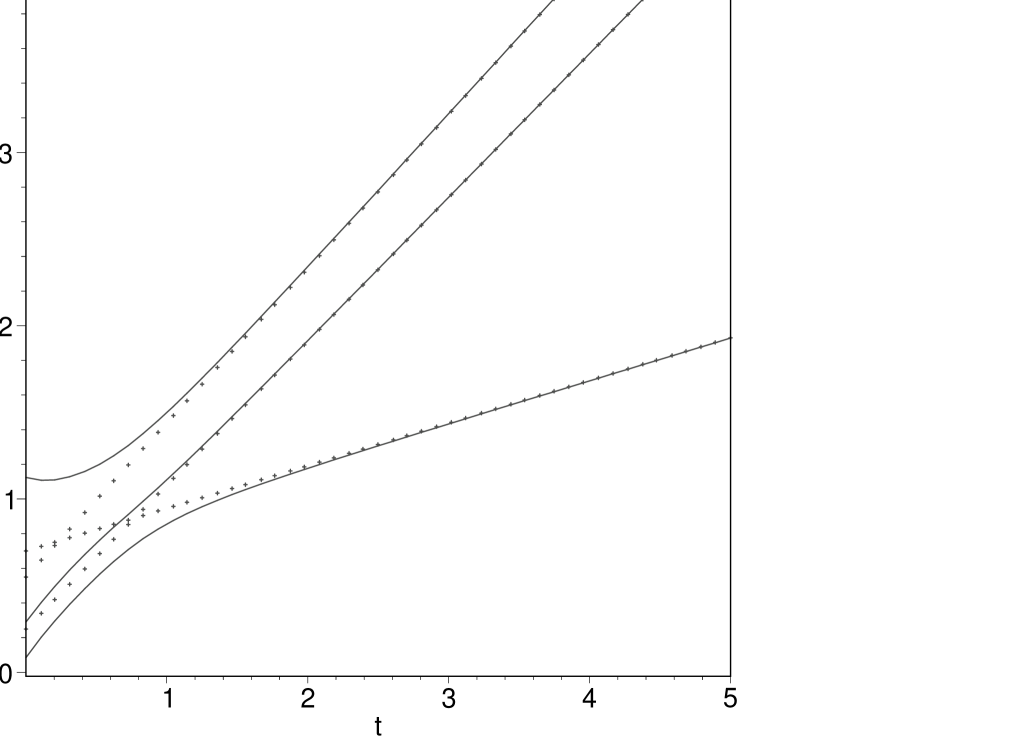
Figure 1: Glueball, $f$ and $f^{\prime}$ Regge trajectories as functions of $t$–channel energy squared $t$ (in $GeV^{2}$). Dotted lines — bare trajectories, solid lines — trajectories with the coupling $g_{ik}(t)$ taken into account in the form (A5.7), with parameters $k=1,\lambda^{2}=\frac{2}{3}GeV^{2}$.

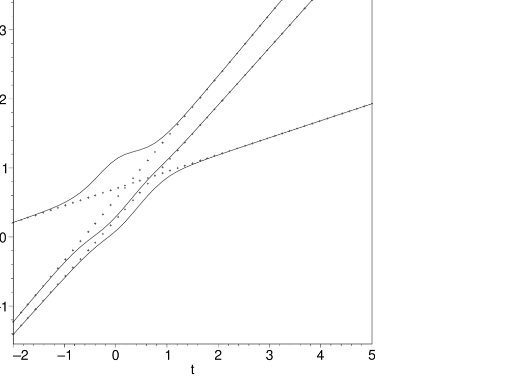
Figure 2: The same as in Fig.1 but for the coupling parameters $k=2,\lambda^{2}=\frac{2}{3}GeV^{2}$.

References

- [1] C.Morningstar, M.Peardon, Nucl. Phys. B (Proc. Suppl.) 63 A-C (19980 22; Phys. Rev. D60 (1999) 034509
-
[2]
G.S.Bali et al. (UK QCD Collaboration), Phys. Lett. B309 (1993)
318;
G.S.Bali, hep-lat/9901023;
G.S.Bali, et al. Nucl. Phys. Proc. Suppl., 63 (1998) 209 - [3] M. Teper, hep-th/9812187
- [4] A.Vaccarino, D.Weingarten, hep-lat/9910007
- [5] K.Peters, in: Hadron Spectroscopy, eds. Suh-Urh Chung, H.J.Willutzki, AIP Conf. Proc. 432, p. 669
- [6] See in: Low–Energy Antiproton Physics, Proc. of the Vth Biennial Conference on Low–Energy Antiproton Physics, Villasimius, 7-12 Sept. 1998, Eds. C.Cicalo, A. De Falco, G.Puddu and S.Serci, North Holland, 1999, Elsevier
- [7] H.Fritzsch and P.Minkowski, Nuovo Cim. A30 (1975) 393; M.Fritzsch and M.Gell–Mann, Proc. 16th Int. Conf. on High–Energy Physics, FNAL 2 (1972) 135
- [8] R.L.Jaffe and K.Johnson, Phys. Lett. B60 (1976) 201
- [9] P.Hasenfrantz and J.Kuti, Phys. Rep. 40 (1978) 75
-
[10]
D.Robson, Nucl. Phys. B130 (1977) 328;
J.M.Cornwall and A.Soni, Phys. Lett. B120 (1983) 431. -
[11]
F.E.Low, Phys. Rev. D12 (1975) 163;
S.Nussinov, Phys. Rev. Lett. 34 (1975) 1286 - [12] V.S.Fadin, E.A.Kuraev, L.N.Lipatov, Sov. Phys. JETP 44 (1976) 443, 45 (1977) 199; I.I.Balitsky, L.N.Lipatov, Sov. J. Nucl. Phys. 28 (1978) 822; L.N.Lipatov, Nucl. Phys. B365 (1991) 614; Sov. Phys. JETP 63 (1986) 904
- [13] Yu.A.Simonov, Nucl. Phys. B307 (1988) 512; Yad. Fiz. 54 (1991) 192
- [14] A.Yu.Dubin, A.B.Kaidalov and Yu.A.Simonov, Phys. Lett. B323 (1994) 41, Yad. Fiz. 56 (1993) 213
- [15] A.Yu.Dubin, A.B.Kaidalov and Yu.A.Simonov, Phys. Lett. B343 (1995) 360, Yad.Fiz. 58 (1995) 348
- [16] Yu.A.Simonov, Phys. Lett. B226 (1989) 151; Z.Phys. 53C (1992) 419
-
[17]
Yu.A.Simonov, Phys.
Lett. B228 (1989) 413;
M.Fabre de la Ripelle and Yu. A.Simonov, Ann. Phys. (N.Y) 212(1991) 235 -
[18]
Yu.A.Simonov, Phys. Lett. B249
(1990) 514;
Yu.A.Simonov, preprint TPI-MINN-90/19-T (unpublished) - [19] V.L.Morgunov, A.V.Nefediev and Yu.A.Simonov, Phys. Lett. B459 (1999) 653; hep-ph/9906318
-
[20]
A.Donnachi and P.V.Landshoff, Nucl. Phys. B244 (1984) 332;
A.B.Kaidalov, L.A.Ponomarev and K.A.Ter-Martirosyan, Sov. J. Phys. 44 (1986) 468 - [21] Yu.A.Simonov, in: Lecture Notes in Physics, Springer, v.479, 1996, p. 139
-
[22]
I.J.Ford, R.H.Dalitz and J.Hoek, Phys. Lett.
B208 (1988) 286;
N.A.Campbell, I.H.Jorysz, C.Michael, Phys. Lett. B167 (1986) 91:
S.Deldar, hep-lat/9809137;
G.Bali, hep-lat/9908021 -
[23]
H.G.Dosch, Phys. Lett. B190 (1987) 177;
H.G.Dosch and Yu.A.Simonov, Phys. Lett. B205 (1988) 339;
for a review see Yu.A.Simonov, Physics Uspekhi 39 (1996) 313 -
[24]
Dan La Course and M.G.Olsson, Phys. Rev. D39 (1989) 2751;
M.G.Olsson, Nuovo Cim. 107 A (1994) 2541 -
[25]
Yu.A.Simonov, Nucl. Phys. B324 (1989) 67;
A.M.Badalian and Yu.A.Simonov, Yad. Fiz. 59 (1996) 2247;
(Phys. At. Nuclei 59 (1996) 2164) - [26] E.Eichten and F.L.Feinberg, Phys. Rev. D23 (1981) 2724
- [27] A.Di Giacomo and H.Panagopoulos, Phys. Lett. B 285 (1992) 133, A.Di Giacomo, E.Meggiolaro, H.Panagopoulos, Nucl. Phys. B 483 (1997) 371, Nucl. Phys. Proc. Suppl. A 54 (1997) 343
-
[28]
T.Barnes, Z.Phys. C10 (1981) 275;
T.Barnes, F.E.Close and S.Monaghan, Phys. Lett. B110 (1982) 159; Nucl.Phys. B198 (1982) 380. -
[29]
E.Eichten et.al. Phys. Rev. D17 (1978) 3090;
W.Lucha, F.Schoeberl and D.Gromes, Phys. Rep. 200 (1991) 127 -
[30]
V.S.Fadin, L.N.Lipatov, Phys. Lett. B429 (1998) 127;
M.Ciafaloni, G.Camici, Phys. Lett. B430 (1998) 349;
S.J.Brodsky et al. JETP Lett. 70 (1999) 155 - [31] Yu.A.Simonov, Phys. Lett. B (in press)
-
[32]
Yu.A.Simonov,
Yad.Fiz. 3 (1966) 630, (Sov.J. Nucl. Phys.
3 (1966) 461)
A.M.Badalian and Yu.A.Simonov, Yad.Fiz. 3 (1966) 1032, 5 (1967) 88 (Sov. J. Nucl. Phys., 3 (1966) 755; 5 (1967) 60)
F.Calogero and Yu.A. Simonov, Phys. Rev. 169 (1968) 789
- [33] G.Veneziano, Nucl.Phys. B108(1976)285
- [34] G.Veneziano, Phys. Lett.43B (1973)413; Nucl.Phys.B74 (1974)365
- [35] Chan Hong-Mo and J.Paton,Phys. Lett.46B (1973)228 Chan Hong-Mo, J.Paton and Tseri Sheund Tsum,Nucl.Phys. B.86 (1975)479
- [36] G.F.Chew and C.Rosenzweig,Phys. Lett.58B (1975)93; Phys. Rev. D12 (1975) 3907; Nucl.Phys. B.104(1976)296
- [37] A.Capella et.al. Phys. Rep. 236 (1994) 225
-
[38]
P.V.Landshoff, hep-ph/9907392;
J.R.Cudell, A.Donnachie, P.V.Landshoff, Phys. Lett. B448 (1999) 281 - [39] L.P.A.Haakman, O.V.Kancheli, J.H.Koch, Nucl. Phys b518 (1998) 275
- [40] V.N.Gribov, ZhETF 57 (1967) 654
- [41] A.B.Kaidalov, Surveys in High Energy Physics, 13 (1999) 265
- [42] R.L.Jaffe, K.Johnson and Z.Ryzak, Ann. Phys. (NY) 168 (1986) 344.
-
[43]
B.S.De Witt, Phys. Rev. 162 (1967) 1195, 1239;
J.Honerkamp, Nucl. Phys. B48 (1972) 269;
G.’tHooft, Nucl. Phys. B62 (1973) 44, Lectures at Karpacz, in: Acta Univ. Wratislaviensis 368 (1976) 345;
L.F.Abbot, Nucl. Phys. 185 (1981) 189