Abstract

We present a calculation of the cross section for the process $p\bar{p}\rightarrow Z^{\prime}_{t}\rightarrow t\bar{t}$, the production of Topcolor $Z^{\prime}_{t}$ with subsequent decay to $t\bar{t}$ in $p\bar{p}$ collisions at $\sqrt{s}=1.8$ TeV. Variations of the cross section with varying assumptions about the model, the resonance width, the parton distributions and the renormalization scale are presented.

1 Topcolor

The large mass of the top quark suggests that the third generation may play a special role in the dynamics of electroweak symmetry breaking. Most models in which this occurs are based upon topcolor [1, 2], which can generate a large top quark mass through the formation of a dynamical $t\bar{t}$ condensate, generated by a new strong gauge force coupling preferentially to the third generation.

In a typical topcolor scheme the QCD gauge group, $SU(3)_{C}$, is imbedded into a larger structure, e.g., $SU(3)_{1}\times SU(3)_{2}$ with couplings $h_{1}$ and $h_{2}$ respectively. $SU(3)_{2}$ ($SU(3)_{1}$) couples to the third (second and first) generation, and $h_{2}>>h_{1}$. The breaking $SU(3)_{1}\times SU(3)_{2}\rightarrow SU(3)_{C}$ produces a massive color octet of bosons, known as “topgluons”, which couple mainly to $b\bar{b}$ and $t\bar{t}$. By itself, this scheme would produce a degenerate top quark and bottom quark. Moreover, if the condensates were required to account for all of EWSB, and without excessive fine-tuning, then the resulting fermion masses would be quite large, $\sim 600$ GeV.

To get the correct scale of the top quark mass one typically considers topcolor in tandem with something else, either an explicit Higgs boson, SUSY, or most naturally with additional strong dynamics, as in “topcolor assisted technicolor” [1]. However, another strategy, which seems very promising, is to invoke a topquark seesaw [3]. In the latter case, the topquark condensate does lead ab initio to a top mass of $\sim 600$ GeV, but through mixing with other electroweak singlet, vector-like fermions the physical top mass is “seesawed” down to its physical value. Again, it is the heaviness of the top quark that makes this latter scheme natural, and minimizes fine tuning. The top quark seesaw seems to emerge naturally in extensions to extra space-time dimensions at the TeV scale [4].

Clearly, all such models require yet another component. Indeed, a “tilting” mechanism is required to enhance the formation of the $t\bar{t}$ condensate, while blocking the formation of the $b\bar{b}$ condensate in all such schemes so that the b-quark is light while top is heavy. This tilting mechanism is constrained by the $\rho$–parameter (or T parameter) because it clearly must violate custodial $SU(2)$

One way to provide the tilting mechanism is to introduce a neutral gauge boson, $Z^{\prime}$, with an attractive interaction between $t\bar{t}$ and a repulsive interaction between $b\bar{b}$. In fact, the $Z$ boson of the Standard Model does precisely this and could itself provide the tilting, however the SM coupling constant $g_{1}$ is so small that one would be fine-tuning to achieve tilting in the presence of a large $h_{2}$. Hence, typically we introduce a new $Z^{\prime}$ boson to drive the tilting.

There are many ways to engineer the tilting with a new $Z^{\prime}$. Obviously anomaly cancellation is mandated for all gauge forces, but this is not a sufficiently powerful constraint to uniquely specify the couplings. The simplest approach is to imbed $U(1)\rightarrow U(1)_{1}\times U(1)_{2}$ in complete analogy to the topcolor imbedding, and each $U(1)_{i}$ is just the appropriate weak hypercharge operator, with $i=2$ ($i=1$) acting on the third (second and first) generation. This produces a topcolor $Z^{\prime}$, the $Z^{\prime}_{t}$, which couples strongly to the third generation and weakly to the first and second, and which, remarkably, can satisfy all of the constraints of flavor changing processes [5] (despite the loss of explicit GIM cancellation).

In the present paper we will consider the physics in production and decay of the $Z^{\prime}_{t}$. In addition to the standard $Z^{\prime}_{t}$ discussed above, which we call Model I, we will present three additional new models of the $Z^{\prime}_{t}$ (Model’s II, III and IV). We will find that the standard $Z^{\prime}_{t}$ from Model I has the lowest production cross section of the four models. Although the standard $Z^{\prime}_{t}$ could be found in this decay channel at the Fermilab Tevatron Collider beginning in the next run, it is more likely to be seen first in the leptonic decay mode at the Tevatron. Models II and III are similar to Model I but yield a higher cross section in the $t\bar{t}$ decay channel. The $Z^{\prime}_{t}$ from Model IV represents a novel class of solutions to the tilting problem. It couples strongly only to the first and third generation of quarks. This $Z^{\prime}_{t}$ from Model IV has no significant couplings to leptons. It is therefore leptophobic and topophyllic.

2 Topcolor $Z^{\prime}$ Models

Standard $Z^{\prime}_{t}$ Production and Decay

(Model I): generation $(3)\supset U(1)_{2}$ and generations $(1,2)\supset U(1)_{1}$

We consider incoherent production, which does not include $\gamma-Z-Z^{\prime}_{t}$ interference terms. This is valid in the narrow width approximation for $Z^{\prime}_{t}$. We use a convention of spin-summing and color-summing both initial and final states. This requires a color-averaged and spin-averaged structure function.

The interaction Lagrangian for the $Z^{\prime}_{t}$ first proposed in [1] is Model I:

$$L^{\prime} = (\frac{1}{2}g_{1}\cot\theta_{H})Z_{t}^{\prime\mu}\left(\frac{1}{3}(\bar{t}_{L}\gamma_{\mu}t_{L}+\bar{b}_{L}\gamma_{\mu}b_{L})+\frac{4}{3}\bar{t}_{R}\gamma_{\mu}t_{R}-\frac{2}{3}\bar{b}_{R}\gamma_{\mu}b_{R}\right.$$ (1)

$$\left.-\bar{\tau}_{L}\gamma_{\mu}\tau_{L}-\bar{\nu_{\tau L}}\gamma_{\mu}\nu_{\tau L}-2\bar{\tau}_{R}\gamma_{\mu}\tau_{R}\right)$$

$$-(\frac{1}{2}g_{1}\tan\theta_{H})Z_{t}^{\prime\mu}\left(\frac{1}{3}(\bar{u}_{L}\gamma_{\mu}u_{L}+\bar{d}_{L}\gamma_{\mu}d_{L})+\frac{4}{3}\bar{u}_{R}\gamma_{\mu}u_{R}-\frac{2}{3}\bar{d}_{R}\gamma_{\mu}d_{R}\right.$$

$$\left.-\bar{e}_{L}\gamma_{\mu}e_{L}-\bar{\nu_{eL}}\gamma_{\mu}\nu_{eL}-2\bar{e}_{R}\gamma_{\mu}e_{R}\right)$$

$$+\left(\makebox{ second generation $\equiv$ first generation }\right)$$

We compute the total cross-section $\sigma(q\bar{q}\rightarrow Z^{\prime}_{t}\rightarrow t\bar{t})$ keeping the top quark mass dependence and spin-summing and color-summing on both initial and final states:

$$\sigma(u+\bar{u}\rightarrow t+\bar{t}) = \frac{9\alpha^{2}\pi}{16\cos^{4}\theta_{W}}\left(\frac{17}{9}\right)\left[\beta(1+\frac{1}{3}\beta^{2})\left(\frac{17}{9}\right)+\frac{8}{9}\beta(1-\beta^{2})\right]\times$$

$$\qquad\times\left[\frac{s}{(s-M_{Z^{\prime}_{t}}^{2})^{2}+s\Gamma^{2}}\right]\theta(s-4m_{t}^{2})$$

and:

$$\sigma(d+\bar{d}\rightarrow t+\bar{t}) = \frac{9\alpha^{2}\pi}{16\cos^{4}\theta_{W}}\left(\frac{5}{9}\right)\left[\beta(1+\frac{1}{3}\beta^{2})\left(\frac{17}{9}\right)+\frac{8}{9}\beta(1-\beta^{2})\right]\times$$

$$\qquad\times\left[\frac{s}{(s-M_{Z^{\prime}_{t}}^{2})^{2}+s\Gamma^{2}}\right]\theta(s-4m_{t}^{2})$$

and in general:

$$\sigma = \frac{9\alpha^{2}\pi}{16\cos^{4}\theta_{W}}\left(\frac{17}{9}\;\makebox{for $u+\bar{u}$;},\;\frac{5}{9}\;\makebox{for $d+\bar{d}$ },\;\frac{5}{3}\;\makebox{for $e+\bar{e}$ or $\mu+\bar{\mu}$ }\right)\times$$

$$\times\left[\beta(1+\frac{1}{3}\beta^{2})\left(\frac{17}{9}\;\makebox{for $t+\bar{t}$;}\right)+\left(\frac{4}{3}\right)\left(\;\frac{5}{9}\;\makebox{for $b+\bar{b}$ };\;\frac{5}{3}\;\makebox{for $\tau+\bar{\tau}$ };\;\frac{1}{3}\;\makebox{for $\nu_{\tau}+\bar{\nu_{\tau}}$ };\right)\right.$$

$$\left.\qquad\qquad+\frac{8}{9}\beta(1-\beta^{2})\;\makebox{(for $t+\bar{t}$)}\right]\times$$

$$\qquad\times\left[\frac{s}{(s-M_{Z^{\prime}_{t}}^{2})^{2}+s\Gamma^{2}}\right]\theta(s-4m_{t}^{2})$$

We obtain the $Z^{\prime}_{t}$ partial decay width to top pairs:

$$\Gamma(Z^{\prime}_{t}\rightarrow t\overline{t})=\frac{\alpha\cot^{2}\theta_{H}}{8\cos^{2}\theta_{W}}\sqrt{M_{Z_{t}^{\prime}}^{2}-4m_{t}^{2}}\left(\frac{17}{9}\left[1-\frac{m_{t}^{2}}{M_{Z^{\prime}_{t}}^{2}}\right]-\frac{8}{3}\left[\frac{m_{t}^{2}}{M_{Z^{\prime}_{t}}^{2}}\right]\right)$$ (5)

The partial width to bottom pairs and $\tau$ and $\nu_{\tau}$ (in the limit $m_{b}\rightarrow 0$):

$$\Gamma(Z^{\prime}_{t}\rightarrow b\overline{b})=\frac{\alpha\cot^{2}\theta_{H}}{8\cos^{2}\theta_{W}}\left(\frac{5}{9}_{b}+\frac{5}{3}_{\tau}+\frac{1}{3}_{\nu\tau}\right)M_{Z^{\prime}_{t}}.$$ (6)

The partial width to first [or second generation] (in the limit $m_{b}\rightarrow 0$):

$$\Gamma(Z^{\prime}_{t}\rightarrow q\overline{q}+\ell\overline{\ell})=\frac{\alpha\tan^{2}\theta_{H}}{8\cos^{2}\theta_{W}}\left(\frac{17}{9}+\frac{5}{9}+\frac{5}{3}+\frac{1}{3}\right)M_{Z^{\prime}_{t}}.$$ (7)

and hence the total width:

$$\Gamma(Z^{\prime}_{t}) = \frac{\alpha M_{Z^{\prime}_{t}}\cot^{2}\theta_{H}}{8\cos^{2}\theta_{W}}\left[\sqrt{1-\frac{4m_{t}^{2}}{M_{Z^{\prime}_{t}}^{2}}}\left(\frac{17}{9}-\frac{41m_{t}^{2}}{9M_{Z^{\prime}_{t}}^{2}}\right)+\left(\frac{5}{9}_{b}+\frac{5}{3}_{\tau}+\frac{1}{3}_{\nu\tau}\right)+\right.$$ (8)

$$\left.\qquad\qquad 2\tan^{4}\theta_{H}\left(\frac{17}{9}+\frac{5}{9}+\frac{5}{3}+\frac{1}{3}\right)\right]$$

$$= \frac{\alpha M_{Z^{\prime}_{t}}\cot^{2}\theta_{H}}{8\cos^{2}\theta_{W}}\left[\sqrt{1-\frac{4m_{t}^{2}}{M_{Z^{\prime}_{t}}^{2}}}\left(\frac{17}{9}-\frac{41m_{t}^{2}}{9M_{Z^{\prime}_{t}}^{2}}\right)+\left(\frac{23}{9}\right)+\tan^{4}\theta_{H}\left(\frac{80}{9}\right)\right]$$

3 Non-Standard Topcolor $Z^{\prime}_{t}$ Production and Decay

(A) Generalized $Z^{\prime}_{t}$ production cross-section Non-standard models can be constructed in which the $U(1)_{Y}\rightarrow U(1)_{1}\times U(1)_{2}$ and the generations are grouped differently:

(Model II): generations $(1,3)\supset U(1)_{2}$ and generation $(2)\supset U(1)_{1}$

(Model III): or generations $(1,2,3)\supset U(1)_{2}$ (analogue of Chivukula-Cohen-Simmons [6] spectator coloron scheme)

as distinct from the usual topcolor in which generations $(1,2)\supset U(1)_{1}$ and generation $(3)\supset U(1)_{2}$. If $h_{2}\gg h_{1}$, then $\cot\theta_{H}\gg 1$ and this preserves the desirable features of having a strong $U(1)$ tilting interaction for the top mass, and now the production of $Z^{\prime}_{t}$ from first generation fermions is enhanced; we’ll neglect limits on such a new object from radiative corrections to $Z$ decay, etc.).

We use a convention of spin-summing and color summing (not averaging) both initial and final states. This requires a color-averaged and spin-averaged structure function.

The dominant part of the interaction Lagrangian for Model II is:

$$L^{\prime}{}_{\bf{II}} = (\frac{1}{2}g_{1}\cot\theta_{H})Z_{t}^{\prime\mu}\left(\frac{1}{3}\bar{t}_{L}\gamma_{\mu}t_{L}+\frac{1}{3}\bar{b}_{L}\gamma_{\mu}b_{L}+\frac{4}{3}\bar{t}_{R}\gamma_{\mu}t_{R}-\frac{2}{3}\bar{b}_{R}\gamma_{\mu}b_{R}\right.$$ (9)

$$+\frac{1}{3}\bar{u}_{L}\gamma_{\mu}u_{L}+\frac{1}{3}\bar{d}_{L}\gamma_{\mu}d_{L}+\frac{4}{3}\bar{u}_{R}\gamma_{\mu}u_{R}-\frac{2}{3}\bar{d}_{R}\gamma_{\mu}d_{R}$$

$$\left.-\bar{\tau}_{L}\gamma_{\mu}\tau_{L}-\bar{\nu_{\tau L}}\gamma_{\mu}\nu_{\tau L}-2\bar{\tau}_{R}\gamma_{\mu}\tau_{R}-\bar{e}_{L}\gamma_{\mu}e_{L}-\bar{\nu_{eL}}\gamma_{\mu}\nu_{eL}-2\bar{e}_{R}\gamma_{\mu}e_{R}\right)$$

The dominant part of the interaction Lagrangian for Model III is:

$$L^{\prime}{}_{\bf{III}} = (\frac{1}{2}g_{1}\cot\theta_{H})Z_{t}^{\prime\mu}\left(\frac{1}{3}\bar{t}_{L}\gamma_{\mu}t_{L}+\frac{1}{3}\bar{b}_{L}\gamma_{\mu}b_{L}+\frac{4}{3}\bar{t}_{R}\gamma_{\mu}t_{R}-\frac{2}{3}\bar{b}_{R}\gamma_{\mu}b_{R}\right.$$ (10)

$$\left.+\frac{1}{3}\bar{u}_{L}\gamma_{\mu}u_{L}+\frac{1}{3}\bar{d}_{L}\gamma_{\mu}d_{L}+\frac{4}{3}\bar{u}_{R}\gamma_{\mu}u_{R}-\frac{2}{3}\bar{d}_{R}\gamma_{\mu}d_{R}\right.$$

$$+\frac{1}{3}\bar{c}_{L}\gamma_{\mu}u_{L}+\frac{1}{3}\bar{s}_{L}\gamma_{\mu}d_{L}+\frac{4}{3}\bar{c}_{R}\gamma_{\mu}u_{R}-\frac{2}{3}\bar{s}_{R}\gamma_{\mu}d_{R}$$

$$-\bar{\tau}_{L}\gamma_{\mu}\tau_{L}-\bar{\nu_{\tau L}}\gamma_{\mu}\nu_{\tau L}-2\bar{\tau}_{R}\gamma_{\mu}\tau_{R}-\bar{e}_{L}\gamma_{\mu}e_{L}-\bar{\nu_{eL}}\gamma_{\mu}\nu_{eL}-2\bar{e}_{R}\gamma_{\mu}e_{R}$$

$$\left.-\bar{\mu}_{L}\gamma_{\mu}\mu_{L}-\bar{\nu_{\mu L}}\gamma_{\mu}\nu_{\mu L}-2\bar{\mu}_{R}\gamma_{\mu}\mu_{R}\right)$$

The non-standard $Z^{\prime}_{t}$ production cross-section $\sigma(q\bar{q}\rightarrow Z^{\prime}_{t}\rightarrow t\bar{t})$ is kinematically identical to the standard $Z^{\prime}_{t}$ case discussed above. The results are:

$$\sigma_{\bf{II}} = \frac{9\alpha^{2}\pi}{16\cos^{4}\theta_{W}}\cot^{4}\theta_{H}\times\left(\frac{17}{9}\;\makebox{for initial state $u+\bar{u}$;},\;\frac{5}{9}\;\makebox{for initial $d+\bar{d}$ }\right)$$

$$\times\left[\beta(1+\frac{1}{3}\beta^{2})\times\left(\frac{17}{9}\;\makebox{for final $t+\bar{t}$ or $u+\bar{u}$;},\;\frac{5}{9}\;\makebox{for final $b+\bar{b}$ or $d+\bar{d}$ }\right)\right.$$

$$+\left.\frac{8}{9}\beta(1-\beta^{2})\;\makebox{(for final $t+\bar{t}$)}\right]\left[\frac{s}{(s-M_{Z^{\prime}_{t}}^{2})^{2}+s\Gamma^{2}}\right]\theta(s-4m_{t}^{2})$$

$$\sigma_{\bf{III}} = \frac{9\alpha^{2}\pi}{16\cos^{4}\theta_{W}}\cot^{4}\theta_{H}\times\left(\frac{17}{9}\;\makebox{for initial $u+\bar{u}$;},\;\frac{5}{9}\;\makebox{for initial $d+\bar{d}$ }\right)$$

$$\times\left[\beta(1+\frac{1}{3}\beta^{2})\times\left(\frac{17}{9}\;\makebox{for final $t+\bar{t}$ or $u+\bar{u}$ or $c+\bar{c}$ ;},\;\frac{5}{9}\;\makebox{for final $b+\bar{b}$ or $d+\bar{d}$ or $s+\bar{s}$ }\right)\right.$$

$$+\left.\frac{8}{9}\beta(1-\beta^{2})\;\makebox{(for final $t+\bar{t}$)}\right]\left[\frac{s}{(s-M_{Z^{\prime}_{t}}^{2})^{2}+s\Gamma^{2}}\right]\theta(s-4m_{t}^{2})$$

The decay kinematics are the same as for standard $Z^{\prime}_{t}$. Hence, for Model II:

$$\Gamma_{\bf{II}}(Z^{\prime}_{t}\rightarrow t\overline{t})=\frac{\alpha\cot^{2}\theta_{H}}{8\cos^{2}\theta_{W}}\sqrt{M_{Z^{\prime}_{t}}^{2}-4m_{t}^{2}}\left(\frac{17}{9}\left[1-\frac{m_{t}^{2}}{M_{Z^{\prime}_{t}}^{2}}\right]-\frac{8}{3}\left[\frac{m_{t}^{2}}{M_{Z^{\prime}_{t}}^{2}}\right]\right)$$ (13)

$$\Gamma_{\bf{II}}(Z^{\prime}_{t}\rightarrow u\overline{u})=\frac{\alpha\cot^{2}\theta_{H}}{8\cos^{2}\theta_{W}}M_{Z^{\prime}_{t}}\left(\frac{17}{9}\right)$$ (14)

$$\Gamma_{\bf{II}}(Z^{\prime}_{t}\rightarrow b\overline{b}\;or\;d\overline{d})=\frac{\alpha\cot^{2}\theta_{H}}{8\cos^{2}\theta_{W}}\left(\frac{5}{9}\right)M_{Z^{\prime}_{t}}.$$ (15)

$$\Gamma_{\bf{II}}(Z^{\prime}_{t}\rightarrow e\overline{e}\;or\;\tau\overline{\tau})=\frac{\alpha\cot^{2}\theta_{H}}{8\cos^{2}\theta_{W}}\left(\frac{5}{3}\right)M_{Z^{\prime}_{t}}.$$ (16)

$$\Gamma_{\bf{II}}(Z^{\prime}_{t}\rightarrow\nu_{e}\overline{\nu_{e}}\;or\;\nu_{\tau}\overline{\nu_{\tau}})=\frac{\alpha\cot^{2}\theta_{H}}{8\cos^{2}\theta_{W}}\left(\frac{1}{3}\right)M_{Z^{\prime}_{t}}.$$ (17)

$$\Gamma_{\bf{II}}(Z^{\prime}_{t}\rightarrow c\overline{c})=\frac{\alpha\tan^{2}\theta_{H}}{8\cos^{2}\theta_{W}}M_{Z^{\prime}_{t}}\left(\frac{17}{9}\right)$$ (18)

$$\Gamma_{\bf{II}}(Z^{\prime}_{t}\rightarrow s\overline{s}\;or\;d\overline{d})=\frac{\alpha\tan^{2}\theta_{H}}{8\cos^{2}\theta_{W}}\left(\frac{5}{9}\right)M_{Z^{\prime}_{t}}.$$ (19)

$$\Gamma_{\bf{II}}(Z^{\prime}_{t}\rightarrow\mu\overline{\mu})=\frac{\alpha\tan^{2}\theta_{H}}{8\cos^{2}\theta_{W}}\left(\frac{5}{3}\right)M_{Z^{\prime}_{t}}.$$ (20)

$$\Gamma_{\bf{II}}(Z^{\prime}_{t}\rightarrow\nu_{\mu}\overline{\nu_{\mu}})=\frac{\alpha\tan^{2}\theta_{H}}{8\cos^{2}\theta_{W}}\left(\frac{1}{3}\right)M_{Z^{\prime}_{t}}.$$ (21)

The partial widths for Model III are the same as Model II, with the replacement $\tan\theta_{H}\rightarrow\cot\theta_{H}$.

We thus have the Model II total width:

$$\Gamma_{\bf{II}} = \frac{\alpha M_{Z^{\prime}_{t}}\cot^{2}\theta_{H}}{8\cos^{2}\theta_{W}}\left[\sqrt{1-\frac{4m_{t}^{2}}{M_{Z^{\prime}_{t}}^{2}}}\left(\frac{17}{9}-\frac{41m_{t}^{2}}{9M_{Z^{\prime}_{t}}^{2}}\right)-\frac{17}{9}+(2+\tan^{4}\theta_{H})\left(\frac{17}{9}+\frac{5}{9}+\frac{5}{3}+\frac{1}{3}\right)\right]$$ (22)

$$= \frac{\alpha M_{Z^{\prime}_{t}}\cot^{2}\theta_{H}}{8\cos^{2}\theta_{W}}\left[\sqrt{1-\frac{4m_{t}^{2}}{M_{Z^{\prime}_{t}}^{2}}}\left(\frac{17}{9}-\frac{41m_{t}^{2}}{9M_{Z^{\prime}_{t}}^{2}}\right)+\left(\frac{63}{9}\right)+\tan^{4}\theta_{H}\left(\frac{40}{9}\right)\right]$$

and the Model III total width:

$$\Gamma_{\bf{III}} = \frac{\alpha M_{Z^{\prime}_{t}}\cot^{2}\theta_{H}}{8\cos^{2}\theta_{W}}\left[\sqrt{1-\frac{4m_{t}^{2}}{M_{Z^{\prime}_{t}}^{2}}}\left(\frac{17}{9}-\frac{41m_{t}^{2}}{9M_{Z^{\prime}_{t}}^{2}}\right)+2\times\frac{17}{9}+3\left(\frac{5}{9}_{d}+\frac{5}{3}_{\ell}+\frac{1}{3}_{\nu\ell}\right)\right]$$ (23)

$$= \frac{\alpha M_{Z^{\prime}_{t}}\cot^{2}\theta_{H}}{8\cos^{2}\theta_{W}}\left[\sqrt{1-\frac{4m_{t}^{2}}{M_{Z^{\prime}_{t}}^{2}}}\left(\frac{17}{9}-\frac{41m_{t}^{2}}{9M_{Z^{\prime}_{t}}^{2}}\right)+\left(\frac{103}{9}\right)\right]$$

Cross-sections are spin-color-summed on both initial and final legs states.

For Model II the cross section is

$$\sigma_{\bf{II}} = \frac{9\alpha^{2}\pi}{16\cos^{4}\theta_{W}}\cot^{4}\theta_{H}\times\left(\frac{17}{9}\;\makebox{for initial state $u+\bar{u}$;},\;\frac{5}{9}\;\makebox{for initial $d+\bar{d}$ }\right)$$

$$\times\left[\beta(1+\frac{1}{3}\beta^{2})\times\left(\frac{17}{9}\;\makebox{for final $t+\bar{t}$ or $u+\bar{u}$;},\;\frac{5}{9}\;\makebox{for final $b+\bar{b}$ or $d+\bar{d}$ };\right.\right.$$

$$\qquad\qquad\left.\left.\;\frac{5}{3}\;\makebox{for final $\tau+\bar{\tau}$ or $e+\bar{e}$ };\;\frac{1}{3}\;\makebox{for final $\nu_{\tau}+\bar{\nu_{\tau}}$ or $\nu_{e}+\bar{\nu_{e}}$ };\right)\right.$$

$$+\left.\frac{8}{9}\beta(1-\beta^{2})\;\makebox{(for final $t+\bar{t}$)}\right]\left[\frac{s}{(s-M_{Z^{\prime}_{t}}^{2})^{2}+s\Gamma^{2}}\right]\theta(s-4m_{t}^{2})$$

(24)

For Model III the cross section is

$$\sigma_{\bf{III}} = \frac{9\alpha^{2}\pi}{16\cos^{4}\theta_{W}}\cot^{4}\theta_{H}\times\left(\frac{17}{9}\;\makebox{for initial $u+\bar{u}$;},\;\frac{5}{9}\;\makebox{for initial $d+\bar{d}$ }\right)$$

$$\times\left[\beta(1+\frac{1}{3}\beta^{2})\times\left(\frac{17}{9}\;\makebox{for final $t+\bar{t}$ or $u+\bar{u}$ or $c+\bar{c}$ ;},\;\frac{5}{9}\;\makebox{for final $b+\bar{b}$ or $d+\bar{d}$ or $s+\bar{s}$ };\right.\right.$$

$$\qquad\qquad\left.\left.\;\frac{5}{3}\;\makebox{for final $\tau+\bar{\tau}$ or $e+\bar{e}$ or $\mu+\bar{\mu}$ };\;\frac{1}{3}\;\makebox{for final $\nu_{\tau}+\bar{\nu_{\tau}}$ or $\nu_{e}+\bar{\nu_{e}}$ or $\nu_{\mu}+\bar{\nu_{\mu}}$};\right)\right.$$

$$+\left.\frac{8}{9}\beta(1-\beta^{2})\;\makebox{(for final $t+\bar{t}$)}\right]\left[\frac{s}{(s-M_{Z^{\prime}_{t}}^{2})^{2}+s\Gamma^{2}}\right]\theta(s-4m_{t}^{2})$$

Dilepton final states are no doubt more sensitive discovery channels than quark dijets, or top for Models I, II and III.

(B) Leptophobic Non-Standard Topcolor $Z^{\prime}_{t}$

Further non-standard models can be constructed for topcolor tilting with a leptophobic interaction. Anomaly cancellation is most easily implemented by having an overall vector-like interaction, but with different generations playing the role of anomaly vector-like pairing. We do not mix with the $U(1)_{Y}$ in these theories, but we do normalize the coupling to the SM coupling $g_{1}$ as a convention.

(Model IV): quark generations $(1,3)\supset U(1)_{2}$

The dominant part of the interaction Lagrangian for Model IV is:

$$L^{\prime}{}_{IV} = (\frac{1}{2}g_{1}\cot\theta_{H})Z_{t}^{\prime\mu}\left(\bar{t}_{L}\gamma_{\mu}t_{L}+\bar{b}_{L}\gamma_{\mu}b_{L}+f_{1}\bar{t}_{R}\gamma_{\mu}t_{R}+f_{2}\bar{b}_{R}\gamma_{\mu}b_{R}\right.$$ (26)

$$\left.-\bar{u}_{L}\gamma_{\mu}u_{L}-\bar{d}_{L}\gamma_{\mu}d_{L}-f_{1}\bar{u}_{R}\gamma_{\mu}u_{R}-f_{2}\bar{d}_{R}\gamma_{\mu}d_{R}\right)$$

Note that for topcolor tilting, we would require the following: $f_{1}>0$ (attractive $\bar{t}t$ channel) and/or $f_{2}<0$ (repulsive $\bar{b}b$ channel). Also, $\cot\theta_{h}>>1$ to avoid fine-tuning.

Hence, the cross-sections (spin-color-summed on both initial and final legs states) for Model IV are

$$\sigma = \frac{9\alpha^{2}\pi}{16\cos^{4}\theta_{W}}\cot^{4}\theta_{H}\times\left((1+f_{1}^{2})\;\makebox{for initial state $u+\bar{u}$;},\;(1+f_{2}^{2})\;\makebox{for initial $d+\bar{d}$ }\right)$$

$$\times\left[\beta(1+\frac{1}{3}\beta^{2})\times\left((1+f_{1}^{2})\;\makebox{for final $t+\bar{t}$ or $u+\bar{u}$;},\;(1+f_{2}^{2})\;\makebox{for final $b+\bar{b}$ or $d+\bar{d}$ }\right)\right.$$

$$+\left.f_{1}\beta(1-\beta^{2})\;\makebox{(for final $t+\bar{t}$)}\right]\left[\frac{s}{(s-M_{Z^{\prime}_{t}}^{2})^{2}+s\Gamma^{2}}\right]\theta(s-4m_{t}^{2})$$

The partial widths for Model IV are

$$\Gamma_{\bf{IV}}(Z^{\prime}_{t}\rightarrow t\overline{t})=\frac{\alpha\cot^{2}\theta_{H}}{8\cos^{2}\theta_{W}}\sqrt{M_{Z^{\prime}_{t}}^{2}-4m_{t}^{2}}\left((1+f_{1}^{2})\left[1-\frac{m_{t}^{2}}{M_{Z^{\prime}_{t}}^{2}}\right]-3f_{1}\left[\frac{m_{t}^{2}}{M_{Z^{\prime}_{t}}^{2}}\right]\right)$$ (28)

$$\Gamma_{\bf{IV}}(Z^{\prime}_{t}\rightarrow u\overline{u})=\frac{\alpha\cot^{2}\theta_{H}M_{Z^{\prime}_{t}}}{8\cos^{2}\theta_{W}}\left((1+f_{1}^{2})\right)$$ (29)

$$\Gamma_{\bf{IV}}(Z^{\prime}_{t}\rightarrow b\overline{b})=\frac{\alpha\cot^{2}\theta_{H}M_{Z^{\prime}_{t}}}{8\cos^{2}\theta_{W}}\left((1+f_{2}^{2})\right)$$ (30)

$$\Gamma_{\bf{IV}}(Z^{\prime}_{t}\rightarrow d\overline{d})=\frac{\alpha\cot^{2}\theta_{H}M_{Z^{\prime}_{t}}}{8\cos^{2}\theta_{W}}\left((1+f_{2}^{2})\right)$$ (31)

The total decay width for Model IV is

$$\Gamma_{\bf{IV}}=\frac{\alpha\cot^{2}\theta_{H}M_{Z^{\prime}_{t}}}{8\cos^{2}\theta_{W}}\left[\sqrt{1-\frac{4m_{t}^{2}}{M_{Z^{\prime}_{t}}^{2}}}\left((1+f_{1}^{2})-(1+f_{1}^{2}+3f_{1})\frac{m_{t}^{2}}{M_{Z^{\prime}_{t}}^{2}}\right)+(3+f_{1}^{2}+2f_{2}^{2})\right]$$ (32)

As a simple parameter scheme, leptophobic, b_r-phobic, top_r-phyllic, take $f_{1}=1$ and $f_{2}=0$:

$$\Gamma_{\bf{IV}}\rightarrow\frac{\alpha\cot^{2}\theta_{H}M_{Z^{\prime}_{t}}}{8\cos^{2}\theta_{W}}\left[\sqrt{1-\frac{4m_{t}^{2}}{M_{Z^{\prime}_{t}}^{2}}}\left(2-5\frac{m_{t}^{2}}{M_{Z^{\prime}_{t}}^{2}}\right)+4\right]$$ (33)

$$\sigma_{\bf{IV}} \rightarrow \frac{9\alpha^{2}\pi}{16\cos^{4}\theta_{W}}\cot^{4}\theta_{H}\times\left(2\;\makebox{for initial state $u+\bar{u}$;},\;(1)\;\makebox{for initial $d+\bar{d}$ }\right)$$

$$\times\left[\beta(1+\frac{1}{3}\beta^{2})\times\left(2\;\makebox{for final $t+\bar{t}$ or $u+\bar{u}$;},\;(1)\;\makebox{for final $b+\bar{b}$ or $d+\bar{d}$ }\right)\right.$$

$$+\left.(1)\beta(1-\beta^{2})\;\makebox{(for final $t+\bar{t}$)}\right]\left[\frac{s}{(s-M_{Z^{\prime}_{t}}^{2})^{2}+s\Gamma^{2}}\right]\theta(s-4m_{t}^{2})$$

4 Cross Section at the Tevatron

The total cross section for $p\bar{p}\rightarrow Z^{\prime}_{t}\rightarrow t\bar{t}$ is

$$\sigma=\int_{0}^{\infty}\frac{d\sigma}{dm}dm$$ (35)

where $d\sigma/dm$, the differential cross section at $t\bar{t}$ invariant mass $m$, is given by

$$\frac{d\sigma}{dm}=\frac{2}{m}\int_{-\ln(\sqrt{s}/m)}^{\ln(\sqrt{s}/m)}dy_{b}\ \tau{\cal L}(x_{p},x_{\bar{p}})\ \hat{\sigma}(q\bar{q}\rightarrow Z^{\prime}_{t}\rightarrow t\bar{t}).$$ (36)

Here $\hat{\sigma}(q\bar{q}\rightarrow Z^{\prime}_{t}\rightarrow t\bar{t})$ is the parton level subprocess cross section. The kinematic variable $\tau$ is related to the initial state parton fractional momenta inside the proton $x_{p}$ and anti-proton $x_{\bar{p}}$ by $\tau=x_{p}x_{\bar{p}}=m^{2}/s$. The boost of the partonic system $y_{b}$ is given by $y_{b}=(1/2)\ln(x_{p}/x_{\bar{p}})$. The partonic “luminosity function” is just the product of parton distribution functions:

$${\cal L}(x_{p},x_{\bar{p}})=q(x_{p},\mu)\bar{q}(x_{\bar{p}},\mu)+\bar{q}(x_{p},\mu)q(x_{\bar{p}},\mu)$$ (37)

where $q(x,\mu)$ ($\bar{q}(x,\mu)$) is the parton distribution function of a quark (anti-quark) evaluated at fractional momenta $x$ and renormalization scale $\mu$.

The subprocess cross sections in equations LABEL:eq_sigma_I, 24, LABEL:eq_sigma_III and LABEL:eq_sigma_IV are for spin and color summing on both initial and final state legs, while most parton distributions assume spin and color averaged on the initial state legs and spin and color summing on the final state legs. Therefore the subprocess cross sections given by equations LABEL:eq_sigma_I, 24, LABEL:eq_sigma_III and LABEL:eq_sigma_IV must be multiplied by a factor of

$$\left(\frac{1}{spins}\right)^{2}\left(\frac{1}{colors}\right)^{2}=\left(\frac{1}{2}\right)^{2}\left(\frac{1}{3}\right)^{2}=\frac{1}{36}$$ (38)

when used with parton distributions from PDFLIB [10] and other standard sources. We have taken this into account when calculating the cross section. we have also used $m_{t}=175$ GeV/c², and $\cos^{2}\theta_{W}=.768$.

5 Width

The minimum width of the $Z^{\prime}_{t}$ depends on which model is chosen. For model I and II the minimum possible width imposed by equations 8 and 22 is around $\Gamma=0.016M$, with the actual minimum value depending on the $Z^{\prime}_{T}$ mass. For Models III and IV there are no minimum widths imposed by equations 23 and 33 respectively. For model I the minimum possible width is of interest, because the cross section increases as the width decreases. Conversely, for models II, III and IV the cross section increases as the width increases, and the minimum possible width is of less interest. All four models permit a width of $\Gamma=0.02M$. This width qualifies as a narrow resonance, since it is significantly less than the CDF detector resolution for $t\bar{t}$. We will also see that this width gives a significant cross section at the Tevatron for model IV, making it experimentally accessible. Therefore, we will concentrate on a width of $\Gamma=0.02M$ for the purpose of comparing cross sections among models and tabulating results. Table 1 shows how this width relates to the fundamental coupling parameter $\cot^{2}\theta_{H}$.

Mass	$\cot^{2}\theta_{H}$ for Model
(GeV/$c^{2}$)	I	II	III	IV
400	4.56	1.78	1.33	3.52
500	3.87	1.66	1.28	3.18
600	3.53	1.59	1.25	3.00
700	3.34	1.55	1.24	2.90
800	3.23	1.52	1.22	2.84
$\infty$	2.87	1.44	1.19	2.64

Table 1: As a function of $Z^{\prime}_{t}$ mass, we tabulate the value of $\cot^{2}\theta_{H}$ for a width of $\Gamma=0.02M$ for models I - IV.

6 Numerical Results for the Tevatron

We have calculated the lowest order cross section for the process $p\bar{p}\rightarrow Z^{\prime}_{t}\rightarrow t\bar{t}$ using a computer program that numerically performs the integrations in equations 35 and 36. The integration in Eq. 35 was performed using the mass interval $M-10\Gamma<m<M+10\Gamma$. For Models I, II, III and IV we used subprocess cross sections  LABEL:eq_sigma_I, 24, LABEL:eq_sigma_III and LABEL:eq_sigma_IV multiplied by the spin-color factor in equation 38. The only parameter of the topcolor model that affects the cross section is the mixing angle $\cot^{2}\theta_{H}$, or equivalently the width $\Gamma$ which is related to it. After the width choice has been made, the only uncertain parameters of the calculation are the choice of parton distributions and renormalization scale $\mu$. For a default parton distribution set we have chosen CTEQ4L [7]. This is a modern parton distribution set appropriate for leading order calculations and is available in PDFLIB [10]. For a default renormalization scale we choose $\mu=m/2$, half the $t\bar{t}$ invariant mass. This scale has the benefit that it reduces to the usual $\mu=m_{t}$ at top production threshold, but also increases with increasing $t\bar{t}$ invariant mass. With these choices, the total cross section for $p\bar{p}\rightarrow Z^{\prime}_{t}\rightarrow t\bar{t}$ for a $Z^{\prime}_{t}$ width of $\Gamma=0.02M$ is tabulated in table 2 and displayed in Fig. 1 for each of Models I through IV.

We have explored the variation in cross section when changing the $Z^{\prime}_{t}$ model, the $Z^{\prime}_{t}$ width, and when changing the parton distributions and renormalization scale. Figure 2 shows that for Model I the cross section is approximately inversely proportional to the width. Figures  3,  4,  5 shows that for Models II through IV the cross section is approximately proportional to the width. The variation in cross section when changing the parton distribution functions is displayed in Fig 6. We have only included parton distributions determined in the 1990’s and extracted at lowest order, appropriate for our lowest order calculation. By coincidence, the choice of CTEQ4L happens to yield a lower cross section than the others and is therefore also a conservative choice. The variation in cross section when increasing or decreasing the renormalization scale is shown in Fig 7.

The cross section for the $Z^{\prime}_{t}$ in Model IV is large enough that it should be possible to observe or exclude this model, for a significant range of masses and widths, using current data from the Tevatron Collider. Preliminary results on a search for narrow resonances decaying to $t\bar{t}$ are available from CDF  [11] and can be used to constrain a $Z^{\prime}_{t}$ from Model IV. We apologize for an error in the predicted cross section for the standard $Z^{\prime}_{t}$ in the preliminary CDF search. The predictions for the $Z^{\prime}_{t}$ presented here supersedes those presented in reference [11]. We eagerly anticipate the next run of the Tevatron Collider, which should be sensitive to the $Z^{\prime}_{t}$ in all the models we have proposed.

Mass	$\sigma(p\bar{p}\rightarrow Z^{\prime}_{t}\rightarrow t\bar{t})$ [pb]
(GeV/$c^{2}$)	Model I	Model II	Model III	Model IV
400	$1.34$	$4.27$	$2.37$	$2.10\times 10^{1}$
450	$1.05$	$3.07$	$1.78$	$1.44\times 10^{1}$
500	$7.23\times 10^{-1}$	$1.98$	$1.18$	$8.97$
550	$4.77\times 10^{-1}$	$1.25$	$7.61\times 10^{-1}$	$5.48$
600	$3.07\times 10^{-1}$	$7.73\times 10^{-1}$	$4.81\times 10^{-1}$	$3.33$
650	$1.94\times 10^{-1}$	$4.76\times 10^{-1}$	$3.00\times 10^{-1}$	$2.01$
700	$1.21\times 10^{-1}$	$2.89\times 10^{-1}$	$1.85\times 10^{-1}$	$1.21$
750	$7.42\times 10^{-2}$	$1.74\times 10^{-1}$	$1.12\times 10^{-1}$	$7.18\times 10^{-1}$
800	$4.47\times 10^{-2}$	$1.03\times 10^{-1}$	$6.70\times 10^{-2}$	$4.22\times 10^{-1}$
850	$2.64\times 10^{-2}$	$6.03\times 10^{-2}$	$3.94\times 10^{-2}$	$2.44\times 10^{-1}$
900	$1.53\times 10^{-2}$	$3.45\times 10^{-2}$	$2.27\times 10^{-2}$	$1.39\times 10^{-1}$
950	$8.64\times 10^{-3}$	$1.93\times 10^{-2}$	$1.27\times 10^{-2}$	$7.72\times 10^{-2}$

Table 2: As a function of $Z^{\prime}_{t}$ mass in Models I-IV, we tabulate the cross section for the process $p\bar{p}\rightarrow Z^{\prime}_{t}\rightarrow t\bar{t}$ at $\sqrt{s}=1.8$ TeV for a $Z^{\prime}_{t}$ width of $\Gamma=0.02M$ using CTEQ4L parton distributions and a renormalization scale $\mu=m/2$. (half the invariant mass of the $t\bar{t}$ system.)

Figure 1: The lowest order cross section for the process $p\bar{p}\rightarrow Z^{\prime}_{t}\rightarrow t\bar{t}$ from table 2.

Figure 2: For Model I we plot the $Z^{\prime}_{t}$ cross section for various widths divided by the cross section for a width $\Gamma=.02M$.

Figure 3: For Model II we plot the $Z^{\prime}_{t}$ cross section for various widths divided by the cross section for a width $\Gamma=.02M$.

Figure 4: For Model III we plot the $Z^{\prime}_{t}$ cross section for various widths divided by the cross section for a width $\Gamma=.02M$.

Figure 5: For Model IV we plot the $Z^{\prime}_{t}$ cross section for various widths divided by the cross section for a width $\Gamma=.02M$.

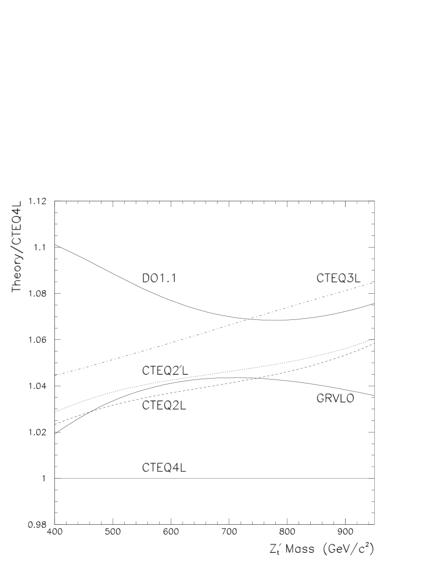
Figure 6: The $Z^{\prime}_{t}$ cross section for Model II with width $\Gamma=0.02M$ for various choices of parton distribution function divided by the cross section with CTEQ4L parton distribution functions. The different choices are CTEQ2L, CTEQ2^′L, CTEQ3L [7], DO1.1 [8] and GRVLO [9].

Figure 7: The $Z^{\prime}_{t}$ cross section for Model II with width $\Gamma=0.02M$ with two other choices of renormalization scale divided by the cross section using renormalization scale $\mu=m/2$. The two choices are $\mu=m$ and $\mu=m/4$.

References

[1] C. T. Hill Phys.
Lett.B266 419, (1991);
Phys. Lett.B345 483 (1995).
[2] C. T. Hill and S. Parke, Phys. Rev. D49 4454 (1994).
[3] B. Dobrescu, C. T. Hill,
Phys. Rev. Lett.81 2634 (1998);
R. Chivukula, B. Dobrescu, H. Georgi,
C. T. Hill, Phys. Rev. D59 075003 (1999).
[4] B. Dobrescu,
Phys. Lett.B461 99 (1999);
H. Cheng, B. Dobrescu, C. T. Hill,
FERMILAB-PUB-99-168-T (June 1999), hep-ph/9906327.
[5] G. Buchalla, G. Burdman, C. T. Hill, D. Kominis,
Phys. Rev.D53 5185 (1996).
[6] R. Chivukula, A. G. Cohen, E. Simmons,
Phys. Lett.B380 92 (1996).
[7] H. L. Lai et al., Phys. Rev. D55, 1280 (1997).
[8] J. F. Owens, Phys. Lett. B266, 126 (1991).
[9] M. Gluck, E. Reya, A. Vogt, Z. Phys. C53, 127 (1992).
[10] H. Plothow-Besch, Comp. Phys. Commun. 75, 396 (1993).
[11] P. Koehn, FERMILAB-CONF-99-306-E, to be published in the
proceedings of International Europhysics Conference on High-Energy Physics
(EPS-HEP 99), Tampere, Finland, 15-21 Jul 1999.