Overall determination of the CKM matrix

Abstract:

We discuss the problem of theoretical uncertainties in the combination of observables related to the CKM matrix elements and propose a statistically sensible method for combining them. The overall fit is performed on present data, and constraints on the matrix elements are presented as well as on $f_{B_{d}}\sqrt{B_{B_{d}}}$. We then explore the implications of recent measurements and developments: ${J\mskip-3.0mu/\mskip-2.0mu\psi\mskip 2.0mu}$$K^{0}_{\scriptscriptstyle S}$ CP asymmetry, $\varepsilon^{\prime}/\varepsilon$ and $B\rightarrow K\pi$ branching fractions. Finally, we extract from the overall fit the Standard Model expectations for the rare kaon decays $K\rightarrow\pi\nu\bar{\nu}$.

1 Introduction

The Cabbibo-Kobayashi-Maskawa (CKM) matrix is extensively studied nowadays. With the birth of the new B factories and the upgrade of the Tevatron experiments, high precision measurements in the B meson sector are expected and the question of testing the CKM ansatz is pushed towards more and more stringent limits. By “testing” we mean two aspects:

1. Given that the Standard Model (SM) is right, what is the best knowledge we have on the CKM free parameters?

2. Are all the measurements involving CKM matrix elements compatible within their errors?

As we shall see (section 2.2), a key point in performing this test is a proper treatment of the theoretical estimates that enter the description of the observables.

First attempts to combine several observables were performed by simply drawing in the Unitarity Triangle (UT) plane individual 95% CL regions for $\rho$ and $\eta$, obtained by varying coherently the experimental and theoretical errors of each observable. These regions had the advantage of being geometrically simple. The intersection of these regions was taken as a 95% CL for ($\rho,\eta)$. While statistically wrong (it neglects the correlations induced by the combination), this method gives surprisingly good results. It can certainly be used to get an insight into the effect on CKM parameters of a given set of observables.

More sophisticated fits have been proposed [1, 2] but, as in the previous case, assuming some flat (or Gaussian) distribution for theoretical parameters.

We propose here a way of decoupling the experimental measurements from the theoretical estimates (section 2.3). It will be illustrated in the ($\bar{\rho}$,$\bar{\eta}$) plane and the $(\sin 2\alpha,~{}\sin 2\beta)$ plane (section 3). The overall fit leads also to constraints on the theoretical parameters $f_{B_{d}}\sqrt{B_{B_{d}}}$ and $B_{K}$  (section 3.4). Recent experimental and theoretical developments are then investigated (section 4). Finally, the impact of B factories is discussed and the SM rare $K$ branching ratios are extracted (section 5).

2 Outline of the method

2.1 Least Squares method

The method exposed here is discussed in more detail in [3]. It can naturally accommodate any new measurements (as in the case of the Fleischer-Mannel bound [4]).

The CKM matrix contains 4 independent parameters, which can be taken as three angles and a phase, or, exhibiting a hierarchy, as the (improved) Wolfenstein parameters: $\lambda,A,\bar{\rho},\bar{\eta}$. The Cabbibo angle is already very well known [5] and $\lambda=\sin\theta_{c}=0.2205$ will be considered as fixed in the following.

Our task is therefore to determine 3 independent parameters, given a set of measurements $Y_{i}=<Y_{i}>\pm\sigma_{i}$ and their theoretical description Y($A,\bar{\rho},\bar{\eta}$).

Considering the two aspects discussed in the introduction, we are naturally lead to use the least squares estimate method. One builds:

$$\chi^{2}(A,\bar{\rho},\bar{\eta})=\sum_{i}\left[\frac{<Y_{i}>-Y(A,\bar{\rho},\bar{\eta})}{\sigma_{i}}\right]^{2}$$ (1)

Minimising the $\chi^{2}$ function:

1. the values of ($A,\bar{\rho},\bar{\eta}$) taken at the minimum of the function provide the least square estimates. Hyper-regions (as the ($\bar{\rho},\bar{\eta}$) projection, i.e. the UT) at a given confidence level can be constructed.

2. To test the compatibility between all measurements (and their theoretical description), one studies the value taken by the function at its minimum, $\chi^{2}_{min}$. When the errors are Gaussian, one can further use the $\chi^{2}$ probability distribution to quantify it.

2.2 The problem with theoretical estimates

Life would be simple if factors that include some level of model dependence did not enter into the calculation. In the following, these will the bag factors for $K$ and $B$ mesons ($B_{K},B_{B}$), the $B$ decay constant ($f_{B}$, which will be combined with the previous bag factor to give $f_{B_{d}}\sqrt{B_{B_{d}}}$) and a large part of the error related to $|V_{ub}|$.

While the error on a measured quantity has a clear statistical meaning, this is not the case for the errors quoted by theorists for their estimates. Here enters a level of subjectivity reflecting a “degree of belief” that the true value lies inside some range [6]. This however may vary from one person to another and is impossible to quantify in terms of a probability distribution function (p.d.f.).

Furthermore, not knowing what the p.d.f. of a given theoretical estimate is makes it impossible to combine with the other estimates on the market.

Finally, a crucial point is that, not knowing where the true value of a parameter lies is not equivalent to taking a flat probability distribution within some bounds. This is not a matter of philosophical discussion; any p.d.f. extracted from a combination using a flat p.d.f. for theoretical estimates is senseless.

2.3 One solution

One method to overcome these problems is the following:

• Determine a “reasonable range” for each theoretical parameter, given the spread of published results. Here reasonable might mean “conservative”.

• Bin the whole range, and scan all the values of the theoretical parameters. For each set of values (a “model”), build and minimise the $\chi^{2}$ (equation 1) using statistical errors only. Since these are Gaussian, one can test the compatibility between the measurements for this set of theoretical values. The estimate is rejected if it does not pass a $Prob(\chi^{2})$ test. If it succeeds, draw a 95% CL contour in the UT plane.

• Now, one does not know which contour is right, but presumably one of them will be correct (assuming the scanned range is really reasonable). Therefore our maximum knowledge is that the set of all these contours is an overall 95% CL. Visually, it corresponds to the envelope of all the individual contours.

The only output of such a method is to provide an overall 95% CL region in the ($\bar{\rho},\bar{\eta}$) plane (or in $(\sin 2\alpha,~{}\sin 2\beta)$). No particular p.d.f. can be inferred, and estimates of the mean and the “$\sigma$” have no particular meaning; the p.d.f. within the envelope is simply unknown.

3 CKM 1999

3.1 Observables

Our present knowledge of the CKM elements lies in the following observables.

3.1.1 $|V_{cb}|$

$|V_{cb}|$ gives a direct access to the $A$ parameter of the Wolfenstein parametrization. Much work on the experimental/theoretical side allows us to quote [8]:

$$|V_{cb}|=0.040\pm 0.002$$ (2)

Note that part of the error quoted here is indeed model-dependent, but it was checked that no “visual” difference can be observed when treating it as a model-dependent range. We can safely consider it as statistical in the following.

3.1.2 $|V_{ub}|$

• there has been a recent update of the CLEO $B\rightarrow\rho\ell\nu$ analysis [7] giving:

  $$|V_{ub}|=[3.25\pm 0.14(stat)^{+0.21}_{-0.29}(syst)$$

  $$\pm 0.55(model)]\times 10^{-3}$$

• also LEP reports a combined value [8]:

  $$|V_{ub}|=[4.05^{+0.39}_{-0.46}(stat+det)^{+0.43}_{-0.51}(b\rightarrow c)$$

  $${}^{+0.23}_{-0.27}(b\rightarrow u)\pm 0.16(HQE)]\times 10^{-3}$$

  where the last three terms corresponds to systematics related to the modelling of $b\rightarrow c$, $b\rightarrow u$ and to the Heavy Quark expansion, used to relate the measured $BR(b\rightarrow X_{u}\ell\nu)$ to $|V_{ub}|$.

The LEP measurements have a statistical error about twice as large as CLEO, and both experiments have the same order of magnitude for detector systematics. But clearly the dominant part of the error is model-dependent. Since it would be questionable to go beyond 15% (relative) error for this term [6] we will use as a reasonable guess estimate:

$$|V_{ub}|=<|V_{ub}|>\pm 0.13\times 10^{-3}(stat)$$

where we will vary the mean within the range:

$$<|V_{ub}|>\in[2.9,3.9]\times 10^{-3}$$ (3)

Note that the final results do not depend crucially on the details of the value used here.

3.1.3 $|\varepsilon_{K}|$

We use for this measurement the PDG value [5]:

$$|\epsilon_{K}|=(2.285\pm 0.018)\times 10^{-3}$$ (4)

The theoretical description of this observable in terms of CKM matrix elements can be found in the literature (see for instance [9]) and requires a value for the non-perturbative QCD bag factor, $B_{K}$. Following Buras [9], we will use:

$$B_{K}\in[0.65,0.95]$$ (5)

3.1.4 ${\Delta{m}_{B_{d}}}$

The LEP oscillation working group has produced an optimal combined value for the B mixing frequency [10]:

$${\Delta{m}_{B_{d}}}=0.473\pm 0.016\,\mbox{ps}^{-1}$$ (6)

Again, theoretical computations require not only a value for the corresponding bag factor $B_{B}$, but also in this case the $B$ decay constant $f_{B}$, so that finally the relevant model-dependent theoretical parameter is $f_{B_{d}}\sqrt{B_{B_{d}}}$.

Here again, opinions may vary on a conservative range. Following the work performed in the B A B AR Physics book [3], we will use:

$$f_{B_{d}}\sqrt{B_{B_{d}}}\in[160,240]\mbox{\,Me\kern-0.80002ptV}$$ (7)

Given the large variations observed with the first unquenched estimates [11], this range may even be over-optimistic.

3.1.5 $\Delta{m}_{B_{s}}$

The study of the mixing frequency in the strange B meson sector has not lead to a firm measurement, but much information can be inferred from the combination of the amplitudes performed by the LEP Oscillation working group [10].

As already detailed in [3] and [4], we use the available information optimally by building a $\chi^{2}$ of the form:

$$\chi^{2}(A,\bar{\rho},\bar{\eta})=\left[\frac{{\cal A}(\Delta{m}_{B_{s}}(A,\bar{\rho},\bar{\eta}))-1}{\sigma_{\cal A}}\right]^{2}$$ (8)

where ${\cal A},\sigma_{\cal A}$ are extracted from the amplitude curve, and $\Delta{m}_{B_{s}}$($A,\bar{\rho},\bar{\eta}$) is the theoretical computation.

It is frequently argued that theoretical errors cancel when taking the ratio $\Delta{m}_{B_{s}}/{\Delta{m}_{B_{d}}}$. This is only true to the level of precision determined by the new theoretical parameter

$$\xi_{s}^{2}=\left[\frac{f_{B_{s}}\sqrt{B_{B_{s}}}}{f_{B_{d}}\sqrt{B_{B_{d}}}}\right]^{2}$$ (9)

For this parameter, we will scan the range ([9] and references therein):

$$\xi_{s}^{2}\in[1.12,1.48]$$ (10)

Measurement	Mean value	Error
$|V_{cb}|$	$.040$	$0.002$
$|V_{ub}|(\times~{}10^{3})$	$<|V_{ub}|>$	$0.13$
$|\epsilon_{K}|(\times~{}10^{3})$	$2.285$	$0.018$
${\Delta{m}_{B_{d}}}$$(\,\mbox{ps}^{-1})$	$0.473$	$0.016$
$\Delta{m}_{B_{s}}$cf.(3.1.5)	${\cal A}$	$\sigma_{\cal A}$

Table 1: The set of measured values used in the global fit. Whenever possible the error is statistical only.

Parameter	Min.	Max.
$<|V_{ub}|>(\times 10^{3})$	2.9	3.9
$B_{K}$	0.65	0.95
$f_{B_{d}}\sqrt{B_{B_{d}}}$( MeV)	160	240
$\xi_{s}^{2}$	1.12	1.48

Table 2: Range scanned in the global fit of the model-dependent theoretical parameters.

3.2 Unitarity Triangle

We build the $\chi^{2}(A,\bar{\rho},\bar{\eta})$ defined in section 1 with all the observables described in the previous part, only using statistical errors (table 1). Each model-dependent parameter is scanned independently within the range of table 2. For each set of these values, the $\chi^{2}$ is minimised using the package MINUIT [12] and the estimate is kept if it satisfies a $\chi^{2}$ probability cut, $P(\chi^{2}_{min})\geq 0.05$. We then draw the associated 95% CL contour in the $(\bar{\rho},\bar{\eta})$ plane, for this model. Each model surviving the cut is superimposed. The envelope of all the contours is the overall 95% CL region for the CKM parameters ($\bar{\rho},\bar{\eta}$).

From figure 1 one can extract (roughly) the projections:

$$0\leq\bar{\rho}\leq 0.3$$ (11)

$$0.2\leq\bar{\eta}\leq 0.45$$ (12)

From such a global fit, an estimate of the third CKM parameter $A$ is possible. However, given the model dependency induced on that parameter by the various observables, it is certainly wiser to extract $A$ directly from the $|V_{cb}|$ measurement alone:

$$A=\frac{|V_{cb}|}{\lambda^{2}}=0.82\pm 0.04$$ (13)

3.3 ($\sin 2\alpha$, $\sin 2\beta$)

The same $\chi^{2}$ can be built in another basis, namely $(A,\sin 2\alpha,\sin 2\beta)$. The same procedure is applied and figure 2 shows the 95% CL region in the $(\sin 2\alpha,\sin 2\beta)$ plane.

From that figure we get the projections (95% CL):

$$.50\leq\sin 2\beta\leq.85$$ (14)

$$-.95\leq\sin 2\alpha\leq.50$$ (15)

The 95% CL regions we obtain are larger than those reported in [2], especially for the $\sin 2\alpha$ parameter. This comes from a (somewhat) different choice of the parameters (mainly $\xi_{sMAX}^{2}$) but especially from a different treatment of the theoretical errors; in [2] the 95% CL region for $\sin 2\alpha$ is extracted from the “p.d.f.” inferred from the fit. As detailed in section 2.2, we disagree with that approach.

3.4 Constraints on $f_{B_{d}}\sqrt{B_{B_{d}}}$

So far, we have just explored the first aspect of testing (getting the best knowledge on the CKM parameters assuming the SM is right) and we turn now to the second; are the results consistent?

Here, recall the procedure; model dependent terms are scanned within a range and for each set of them, the $\chi^{2}$ is computed. The value of the $\chi^{2}$ at its minimum indicates the consistency of all measurements for that set of theoretical parameters. One can therefore reject sets of values which are inconsistent with all the measurements (if they were all rejected, we would conclude there is a consistency problem, implying new physics).

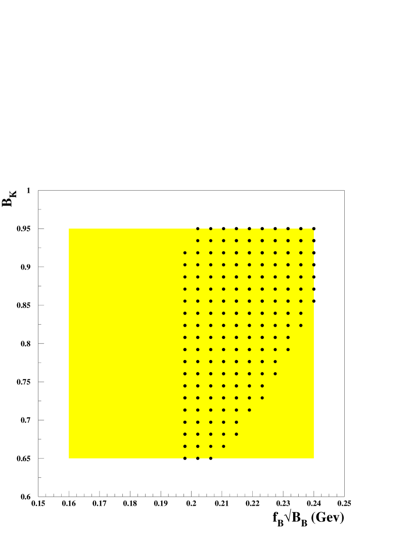
Figure 3: The projection on the $f_{B_{d}}\sqrt{B_{B_{d}}},B_{K}$ plane of the theoretical models that survive the consistency cut of 5% (points). The grey area depicts the whole range scanned.

Figure 3 shows a projection of all the scanned points that survived the $Prob(\chi^{2}_{min})$ cut of 5% during the combination in the ($f_{B_{d}}\sqrt{B_{B_{d}}},B_{K}$) plane. (Note these parameters are somewhat related by lattice computations.)

Figure 3 indicates that the Standard Model combination implies:

• $f_{B_{d}}\sqrt{B_{B_{d}}}\geq 195\mbox{\,Me\kern-0.80002ptV}$

• low values of $B_{K}$ with large values of $f_{B_{d}}\sqrt{B_{B_{d}}}$ are disfavoured

4 Recent developments

4.1 $a_{\psi K_{S}}$ (CDF)

CDF has reported a first measurement of the ${J\mskip-3.0mu/\mskip-2.0mu\psi\mskip 2.0mu}$$K^{0}_{\scriptscriptstyle S}$ CP asymmetry, which leads to the (model-independent) measurement [13]:

$$\sin 2\beta=0.79^{+0.41}_{-0.44}$$ (16)

With respect to what is already known on $\sin 2\beta$ from the combination above (figure 2), it clearly does not constrain the CKM matrix elements any further.

This is however the first measurement directly related to the phases of the CKM matrix only and the fact that $\sin 2\beta>0$ (95% CL) is strong support for the validity of the CKM description.

4.2 $\varepsilon^{\prime}/\varepsilon$ (KTeV, NA48)

A large value for this observable has been measured by the KTeV and NA48 collaborations. Their combination gives [14]

$$\varepsilon^{\prime}/\varepsilon=(21.3\pm 2.8)\times 10^{-4}$$ (17)

The CKM description of this observable involves only $\eta$:

$$\varepsilon^{\prime}/\varepsilon=\eta A^{2}\lambda^{5}F_{\epsilon^{\prime}}$$ (18)

but the function $F_{\epsilon^{\prime}}$ includes many theoretical factors. A crude description is [15]:

$$F_{\epsilon^{\prime}} = 13\left[\frac{110\mbox{\,Me\kern-0.80002ptV}}{m_{s}(m_{c})}\right]^{2}\times\frac{\Lambda_{\bar{MS}}^{(4)}}{340\mbox{\,Me\kern-0.80002ptV}}$$ (19)

$$\times[{B_{6}^{(1/2)}}(1-\Omega_{\eta+\eta^{\prime}})-0.4B_{8}^{(3/2)}\left(\frac{m_{t}(m_{t})}{165\mbox{\,Ge\kern-0.80002ptV}}\right)^{2.5}]$$

The main uncertainties in this formula are related to the QCD penguins ($B_{6}^{(1/2)}$), electroweak penguins ($B_{8}^{(3/2)}$) and the strange quark mass ($m_{s}(m_{c})$).

The difficulty in predicting any value for this parameter comes from the fact that two badly known parameters ($B_{6}^{(1/2)}$ and $B_{8}^{(3/2)}$) are subtracted and that the difference could be as low as 0. On the other hand, this difference cannot be too large. And an upper bound on $F_{\epsilon^{\prime}}$ directly translates into a lower bound on $\eta$ (equation 18). For instance using [15]: $B_{6}^{(1/2)}=1.0\pm 0.3,B_{8}^{(3/2)}=0.8\pm 0.2,m_{s}(m_{c})=130\pm 25\mbox{\,Me\kern-0.80002ptV}$, $\Lambda_{\bar{MS}}^{(4)}=340\pm 50\mbox{\,Me\kern-0.80002ptV},\Omega_{\eta+\eta^{\prime}}=0.25\pm 0.08,m_{t}=165\pm 5\mbox{\,Ge\kern-0.80002ptV}$ and coherently varying the errors, one obtains:

$$F_{\epsilon^{\prime}}\leq 13.4$$ (20)

which translates into:

$$\eta\geq\frac{\varepsilon^{\prime}/\varepsilon}{13.4|V_{cb}|^{2}\lambda}$$ (21)

and using the experimental input (sections 2 and 17), allowing a 2$\sigma$ variation, one obtains:

$$\eta\geq 0.32$$ (22)

Given figure 1 this would be a strong constraint on the UT.

Unfortunately, the formula (equation 19) is not accurate enough. But the message is; since the measurements provide a large value of $\varepsilon^{\prime}/\varepsilon$, a firm upper bound on the theoretical parameters can be enough to constrain significantly the $\eta$ parameter of the CKM matrix.

4.3 Bounds from $B\rightarrow K\pi$

4.3.1 The “Fleischer-Mannel bound”

Fleischer and Mannel have proposed [16] a constraint on the angle $\gamma$ of the UT, solely from the measurements of $C\!P$-averaged branching ratio $B\rightarrow K\pi$:

$$\sin^{2}\gamma\leq R$$ (23)

where

$$R=\frac{\Gamma(B_{d}\to\pi^{\mp}K^{\pm})}{\Gamma(B^{\pm}\to\pi^{\pm}K^{0})}$$ (24)

While there has been a lot of discussion about possible theoretical uncertainties that would weaken this bound [17], it suffers mainly from the present CLEO measurement which gives a value of $R$ consistent with one [19]:

$$R=1.11^{+0.35}_{-0.31}$$ (25)

It will certainly worth revisiting it when more accurate measurements become available.

4.3.2 The “Neubert-Rosner bound”

Following that idea, Neubert and Rosner have proposed a bound on $\gamma$ from charged $B$ decays only, in which theoretical uncertainties are much more under control [18]. It relies on two absolute branching ratios, which are used to define:

$$R_{\ast}=\frac{\Gamma(B^{\pm}\rightarrow\pi^{\pm}K^{0})}{2(B^{\pm}\rightarrow\pi^{0}K^{\pm})}$$ (26)

and

$$\bar{\epsilon}_{3/2}=\sqrt{2}R_{SU(3)}\tan\theta_{C}\left[\frac{\Gamma(B^{\pm}\rightarrow\pi^{\pm}\pi^{0})}{\Gamma(B^{\pm}\rightarrow\pi^{\pm}K^{0})}\right]^{\frac{1}{2}}$$ (27)

where in this second formula, $\theta_{C}$ is the Cabbibo angle and $R_{SU(3)}$ is a precisely known correction [20]. Using these observables the bound reads [21]:

$$|X_{R}|=|\frac{\sqrt{R_{\ast}^{-1}}-1}{\bar{\epsilon}_{3/2}}|\leq|\delta_{EW}-{\cos\gamma}|$$ (28)

where $\delta_{EW}$ is calculable in terms of Standard Model parameters:

$$\delta_{EW}=(0.64\pm 0.09)\times\frac{0.085}{|\frac{|V_{ub}|}{|V_{cb}|}|}$$ (29)

The bound in equation 28 is discriminant provided that $X_{R}$ is (statistically) below one. While the first CLEO results were promising, the latest updates [19] do not confirm a value statistically different from one:

$$X_{R}=0.72\pm 0.98(exp)\pm 0.03(th)$$ (30)

As in the Fleischer-Mannel case, one waits eagerly for more precise measurements from CLEO-III, Belle and B A B AR.

5 Future measurements

5.1 B factories

With the start of $B$ factories, one can expect some new measurements of $C\!P$ asymmetries which are related to $\sin 2\beta$ and $\sin 2\alpha$. The stakes are however different. Given figure 2:

• $\sin 2\beta$ is already well constrained. The goal of measuring it is to test the SM, since in a variety of models new physics may appear only in the CKM phases [22]. It is not expected that measuring this angle will constrain $f_{B_{d}}\sqrt{B_{B_{d}}}$ much more than presently.

• $\sin 2\alpha$ is largely unknown and the goal of $B$ factories is to measure it. The extraction of that angle from the measured $C\!P$ asymmetries is difficult (impossible?) and will certainly require several years of running [3]. The most promising channel is presently $B\rightarrow 3\pi$ in which all the amplitudes can be extracted from a global fit to the Dalitz plot.

5.2 $K\rightarrow\pi\nu\bar{\nu}$

Both the charged mode and the neutral one are “theoretically clean” and measuring their rate would significantly constrain the CKM matrix [9]. For the time being, we can extract the expected branching ratio from the global fit by scanning all the points in the contours of figure 1 and keeping the minimum and maximum value of the corresponding computed branching ratio. One obtains (for 95% CL):

$$BR(K_{L}\rightarrow\pi^{0}\nu\bar{\nu}) \in [1-5]\times 10^{-11}$$ (31)

$$BR(K^{+}\rightarrow\pi^{+}\nu\bar{\nu}) \in [4-10]\times 10^{-11}$$ (32)

6 Conclusions

We want to draw the attention of the reader to the difficulties that arise when including some theoretical estimates into an overall combination of observables relevant to the CKM determination. This was also emphasised by Stone [6] and will (and already does) limit our understanding of the CKM parameters. Given that a “theoretical” error has an unclear statistical meaning, we conclude that extracting any p.d.f. from a combination including these parameters is just meaningless, and that no “central values” and “errors” should be ever quoted.

Nevertheless, we have proposed a (conservative) method to obtain some 95% CL regions for all CKM parameters, by separating the statistical errors due to measurements from the systematic and model-dependent ones. From such a combination, we obtain the 95% CL bounds:

• $0\leq\bar{\rho}\leq 0.3,~{}0.2\leq\bar{\eta}\leq 0.45$

• $.50\leq\sin 2\beta\leq.85,~{}-.95\leq\sin 2\alpha\leq.50$

• $f_{B_{d}}\sqrt{B_{B_{d}}}\geq 195\mbox{\,Me\kern-0.80002ptV}$

Among new developments, the large value measured for $\varepsilon^{\prime}/\varepsilon$ could constrain $\eta$ (by a lower bound) if theoretical uncertainties were more under control (an upper bound would be sufficient).

$B\rightarrow K\pi$ absolute branching ratios could constrain significantly the angle $\gamma$ of the UT but must be measured more precisely.

Finally, from the overall combination, one can extract the expected branching ratios:

$$BR(K_{L}\rightarrow\pi^{0}\nu\bar{\nu}) \in [1-5]\times 10^{-11}$$

$$BR(K^{+}\rightarrow\pi^{+}\nu\bar{\nu}) \in [4-10]\times 10^{-11}$$

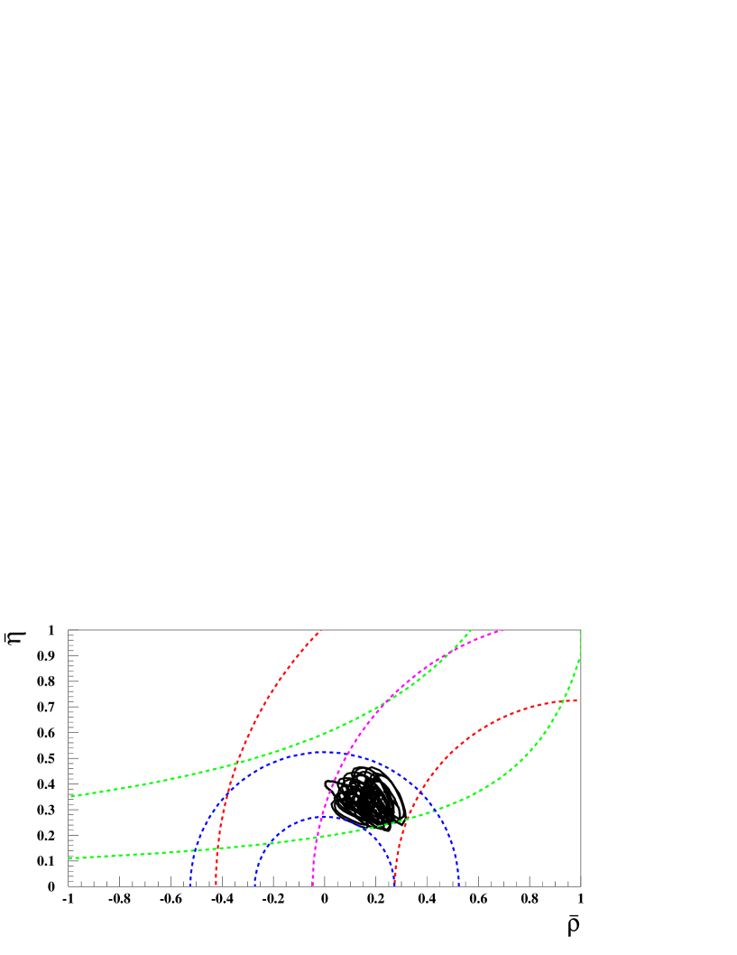
Figure 1: The allowed 95% CL region for $\bar{\rho}$-$\bar{\eta}$. Each contour corresponds to one theoretical model, and the envelope of all of them is the overall 95% CL combination. Also shown (for historical reasons) the usual individual constraints.

Figure 2: The 95% CL allowed region for $\sin 2\alpha$-$\sin 2\beta$. Each contour corresponds to one theoretical model, and the envelope of all of them is the overall 95% CL combination.