OHSTPY-HEP-T-99-020
November 1999

Fermion Masses and Neutrino Oscillations

in $SO(10)$ SUSY GUT with $D_{3}\times U(1)$

Family Symmetry

Radovan Dermíšek and Stuart Raby

Department of Physics, The Ohio State University, 174 W. 18th Ave., Columbus, Ohio 43210

Abstract

Discrete nonabelian gauge symmetries appear to be the most advantageous candidates for a family symmetry. We present a predictive $SO(10)$ SUSY GUT model with $D_{3}\times U(1)$ family symmetry ($D_{3}$ is the dihedral group of order 6). The hierarchy in fermion masses is generated by the family symmetry breaking $D_{3}\times U(1)\rightarrow Z_{N}\rightarrow$ nothing. This model fits the low energy data in the charged fermion sector quite well and naturally provides large angle $\nu_{\mu}$ – $\nu_{\tau}$ mixing describing atmospheric neutrino oscillation data and small angle $\nu_{e}$ – $\nu_{s}$ mixing consistent with the small mixing angle MSW solution to the solar neutrino data. In addition, the non-abelian family symmetry $D_{3}$ is sufficient to suppress large flavor violations.

1 Introduction

The origin of the fermion mass hierarchy is one of the most challenging problems in elementary particle physics. In the standard model fermion masses and mixing angles are free parameters. Even though these 13 parameters (9 charged fermion masses; 3 angles and 1 phase in the CKM matrix) are well known experimentally, the standard model does not offer any explanation. Supersymmetric [SUSY] Grand Unified Theories [GUTs] besides gauge coupling unification also provide relations between quark and lepton masses within generations. However, the understanding of the hierarchy between generations is still missing. A possible solution to the fermion mass hierarchy problem is to introduce a new symmetry – family symmetry – acting horizontally between generations. The hierarchy is then generated by sequential spontaneous breaking of this symmetry. Furthermore, acting differently on different generations, family symmetries can provide a solution to the problem of large flavor changing neutral currents [FCNCs] in SUSY [1].

A variety of models [2] – [9] with family symmetries were proposed. Among these, models with $U(2)$ (or its subgroups) family symmetry [5] –  [9] appear to be very promising candidates for the theory of flavor. The reason for this is twofold: the top quark is the only fermion with mass of order the weak scale, thus distinguishing the third generation from the others; and by placing the first and second generations into a two dimensional irreducible representation of the family group the degeneracy of squarks in these two generations can be achieved, which is necessary to suppress FCNCs. Thus non-Abelian family symmetries, especially $U(2)$ or its subgroups, are naturally suggested.

We would like to focus here on a particular model presented in [7]. It is an $SO(10)$ SUSY GUT with family symmetry $U(2)\times U(1)$. This model is “predictive” by which we mean that it is “natural” – the Lagrangian contains all terms consistent with the symmetries and particle content of the theory; and the number of arbitrary parameters is less than the number of observables. This model fits the low energy data in the charged fermion sector quite well and naturally provides large angle $\nu_{\mu}$ – $\nu_{\tau}$ mixing describing atmospheric neutrino oscillation data and small angle $\nu_{e}$ – $\nu_{s}$ mixing consistent with the small mixing angle MSW solution to solar neutrino data.

There are however complications associated with a $U(2)$ family symmetry in supersymmetric theories. It is believed that global symmetries do not arise in string theory and also these are thought to be violated by quantum gravity effects [10]. On the other hand, with continuous gauge symmetries there are associated D – term contributions to scalar masses which can lead to unacceptably large FCNCs [11]. As a result, we should consider discrete family gauge symmetries. Discrete gauge symmetries are not violated by quantum gravity effects [12] and can arise in spontaneous breaking of continuous gauge symmetries or directly in compactifications of string theory.

In this paper we present an $SO(10)$ SUSY GUT with $D_{3}\times U(1)$ family gauge symmetry which does not suffer from the problems mentioned in the previous paragraph. This model provides exactly the same operators generating Yukawa matrices as model [7]. Thus it fits the low energy data in the charged lepton sector equally well and provides the same neutrino solution. In addition, the field content of this model is simpler than [7] and can naturally provide an explanation for sequential family symmetry breaking by the vacuum expectation values [vevs] of “flavon” fields.

The rest of the paper is organized as follows. In section 2 we briefly review possible discrete family symmetries, provide a motivation for $D_{3}\times U(1)$ as a family symmetry and discuss anomalies associated with gauging of this symmetry. In section 3 we construct the $SO(10)\times D_{3}\times U(1)$ invariant superspace potential which, after family symmetry breaking, generates the quark and lepton Yukawa matrices. Our conclusions are in section 4. For convenience, in Appendix A we summarize properties of the group $D_{3}$ and its representations, and calculate invariants used in section 3. In Appendix B we present a $D^{\prime}_{3}$ version of the model and finally in Appendix C we briefly review the results of  [7] for charged fermion masses and mixing angles as well as for neutrino oscillations.

2 Discrete Family Symmetry

As mentioned in the introduction, we are interested in discrete family symmetries which posses two-dimensional irreducible representations. In order to be able to generate the same operators for fermion masses as in the case of $U(2)$, family symmetry [7] subgroups of $SO(3)$ or $SU(2)$ are suggested.

Discrete subgroups of $SO(3)$ are classified [13] in terms of two infinite series: $Z_{N}$ (cyclic Abelian groups) and $D_{N}$ (non-Abelian dihedral groups); and three exceptional groups: $T$ (tetrahedral), $O$ (octohedral) and $I$ (icosahedral). Similarly, since $SO(3)\cong SU(2)/Z_{2}$, discrete subgroups of $SU(2)$ are classified in terms of double covers of the corresponding subgroups of $SO(3)$. We call these $Z^{\prime}_{N}$, $D^{\prime}_{N}$, $T^{\prime}$, $O^{\prime}$ and $I^{\prime}$. Since $Z_{N}$ are abelian they posses only singlet irreducible representations. Irreducible representations of dihedral groups $D_{N}$ and $D^{\prime}_{N}$ are all one and two dimensional. Three dimensional irreducible representations start to appear in the exceptional groups.

In paper [7] the three generations of fermions transform as a doublet and singlet under $SU(2)$. To generate the effective mass operators for quarks and leptons in the light two generations, three “flavon” fields $\phi^{a}$, $S^{ab}$ and $A^{ab}$ (doublet, symmetric triplet and anti-symmetric singlet under $SU(2)$) were introduced. The family symmetry is sequentially broken by minimal symmetry breaking vevs:

$$\langle\phi^{a}\rangle\;=\;\left(\begin{array}[]{c}0\\ \phi\\ \end{array}\right)\;,\quad\langle S^{ab}\rangle\;=\;\left(\begin{array}[]{cc}0&0\\ 0&S\\ \end{array}\right)\;,\quad\langle A^{ab}\rangle\;=\;\left(\begin{array}[]{cc}0&A\\ -A&0\\ \end{array}\right)\;.$$ (1)

Thus, it looks like we need to consider a group which has at least one three dimensional irreducible representation to have a discrete analog of $S^{ab}$. In that case the tetrahedral group $T^{\prime}$ would be the smallest group we could consider.  However, the coupling of a triplet to two doublets, which is necessary in [7], can be easily mimicked by a coupling of three doublets in most of the dihedral groups. (In the case of $D_{3}$ see eqn. (46) in Appendix A and in the case of $D^{\prime}_{3}$ eqn. (51) in Appendix B.) Therefore a flavon field in the three-dimensional representation is not necessary when considering a dihedral family symmetry. Furthermore, it has not been possible to find a mechanism for generating non-zero vevs for $S^{22}$, while $\langle S^{11}\rangle=\langle S^{12}\rangle=0$ [14]. On the other hand, if the most general family symmetry breaking vevs $\langle S^{11}\rangle=\kappa_{1}S$, $\langle S^{12}\rangle=\kappa_{2}S$ are considered  the predictivity of the theory is lost, since there are now as many parameters in the charged fermion sector as there are observables [15].

Therefore, dihedral groups are the most promising candidates for an “$SU(2)$-like” family symmetry. They were previously used as family symmetries in refs. [8]. If we now demand the minimal family symmetry group containing representations which can be used most economically, we are lead to the group $D_{3}$.

The group $D_{3}$ is the smallest non-Abelian group (it is isomorphic to $S_{3}$ - the symmetric permutation group). Some basic properties of this group and its representations are summarized in Appendix A. $D_{3}$ possesses three nonequivalent irreducible representations ${\bf 1_{A}}$, ${\bf 1_{B}}$ and ${\bf 2_{A}}$ (${\bf 1_{A}}$ is a trivial representation; also denoted by $1$). Thus this symmetry provides a natural interpretation of the three generations of fermions as a singlet and doublet ${\bf 1_{B}}$ + ${\bf 2_{A}}$ under $D_{3}$. Differences between generations can then be understood as a consequence of assigning them to different representations of $D_{3}$.

Since we want the family symmetry to be gauged, it must be anomaly free. To show that there are no combined $D_{3}$ and/or $SO(10)$ anomalies we use the fact that both the $SO(3)$ and $SO(10)$ groups are anomaly free. Representations of $SO(3)$ decompose into irreducible representations of $D_{3}$ in the following way:

$${\bf 1} \rightarrow {\bf 1_{A}}\;,$$

$${\bf 3} \rightarrow {\bf 1_{B}}\;+\;{\bf 2_{A}}\;,$$ (2)

$${\bf 5} \rightarrow {\bf 1_{A}}\;+\;{\bf 2_{A}}\;+\;{\bf 2_{A}}\;,$$

$$\vdots$$

Therefore, if the field content of the theory is such that fields with the same $SO(10)$ quantum numbers can be arranged into complete multiplets of $SO(3)$ then there are no $D_{3}$, $SO(10)$ or mixed anomalies.

Because $D_{3}$ has only two nonequivalent nontrivial irreducible representations we also need (in order to maintain “naturalness”) an additional $U(1)$ symmetry to distinguish different fields with the same $D_{3}$ and $SO(10)$ charges. This $U(1)$ symmetry is in general anomalous. An anomalous $U(1)$ gauge symmetry was previously used in models [3]. We shall assume that the $U(1)$ anomalies can be cancelled by the Green – Schwarz mechanism [16].

Before we continue, it is important to discuss the consequences of the symmetry group $D_{3}$ with regards to flavor violation [1]. It has been shown that an SU(2) family symmetry can effectively suppress flavor violating processes among the first two families [5, 6]. This follows from the fact that to zeroth order in family symmetry breaking, the soft SUSY breaking mass term for squarks and sleptons in the first two families is an SU(2) invariant and thus proportional to the identity matrix. Then family symmetry breaking corrections to squark and slepton masses are at most of order the family mixing for quarks and leptons. In appendix A, we show that the same argument also applies for $D_{3}$. Thus $D_{3}$ will also suppress flavor violations.

3 An $SO(10)\times D_{3}\times U(1)$ Model

In this section we present an $SO(10)$ SUSY GUT with $D_{3}\times U(1)$ family gauge symmetry. In $SO(10)$ all fermions in one generation are contained in the 16 dimensional irreducible representation and, in the simplest version, one pair of Higgs doublets is contained in the 10 dimensional irreducible representation. The minimal Yukawa coupling of the third generation of fermions to the Higgs fields is given by $\lambda 16_{3}1016_{3}$ from which we obtain the symmetry relation $\lambda_{t}=\lambda_{b}=\lambda_{\tau}=\lambda_{\nu_{\tau}}=\lambda$ at the GUT scale. While this Yukawa unification is known to work quite well for the third generation it fails for the two light generations. Thus a family symmetry is necessary to forbid the tree level Yukawa coupling of the first and second generations to the Higgs fields. Breaking of this symmetry will provide the necessary hierarchy of fermion masses.

3.1 The charged fermion sector

As discussed in section 2 the first two generations of fermions are contained in $16_{a}$, $a=1,2$ which is a doublet under $D_{3}$ with charge $1$ under $U(1)$ [ or $16_{a}=({\bf 2_{A}},1)$ ]. The third generation $16_{3}$ transforms as $({\bf 1_{B}},3)$ and a $10$ of Higgs transforms as $(1,-6)$. Using the results of Appendix A we see that the coupling $\lambda 16_{3}1016_{3}$ is invariant under $D_{3}\times U(1)$ while $\lambda 16_{a}1016_{a}$ and $\lambda 16_{a}1016_{3}$ are not.

To generate the Yukawa couplings for the first two generations we introduce three “flavon” superfields:

$$\phi_{a}=({\bf 2_{A}},-2)\;,\quad\tilde{\phi}_{a}=({\bf 2_{A}},-4)\;,\quad A=({\bf 1_{B}},4)\;,$$

which are $SO(10)$ singlets, and a pair of Froggatt-Nielsen states [17] ($\overline{16}$ and $16$ under $SO(10)$):

$$\bar{\chi}_{a}=({\bf 2_{A}},-5)\;,\quad\chi_{a}=({\bf 2_{A}},5)\;.$$

The superspace potential for the charged fermion sector of this model is given by:

$$W\supset\;\; 16_{3}\;10\;16_{3} +\;\;16_{a}\;10\;\chi_{a}$$

$$+ \bar{\chi}_{a}\;(\;M\;\chi_{a} +\;\;\frac{1}{M_{0}}\;45\;\tilde{\phi}_{a}16_{3}\;\;+\;\;\frac{1}{M_{0}}\;45\;\phi_{a}16_{a}\;\;+\;\;A\;16_{a}\;)\;,$$ (3)

where $45=(1,6)$ is an $SO(10)$ adjoint field  which is assumed to obtain a vev in the B – L direction; and $M=(1,0)$ is a linear combination of an $SO(10)$ singlet and adjoint. Its vev $M_{0}(1+\alpha X+\beta Y)$ gives mass to Froggatt-Nielsen states. Here $X$ and $Y$ are elements of the Lie algebra of $SO(10)$ with $X$ in the direction of the $U(1)$ which commutes with $SU(5)$ and $Y$ the standard weak hypercharge; and $\alpha$ , $\beta$ are arbitrary constants which are fit to the data. Furthermore, each term in $W$ has an arbitrary coupling constant which is omitted for notational simplicity. 

The largest scale of the theory is assumed to be the mass of the Froggatt-Nielsen states. In the effective theory below $M_{0}$, these states are integrated out giving the effective mass operators in Figure 1.

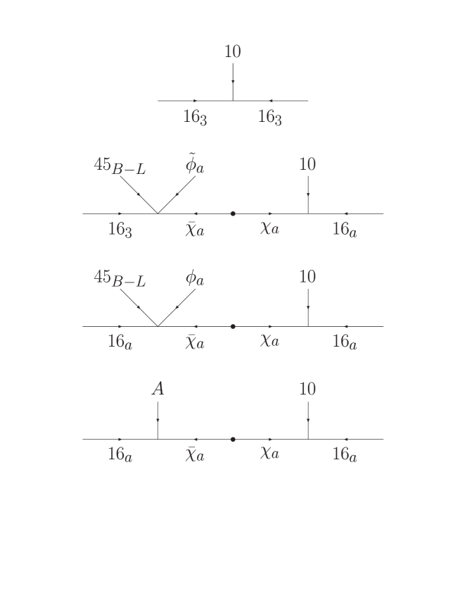
Figure 1: Diagrams generating the Yukawa matrices.

When “flavon” doublets obtain vevs $\langle\tilde{\phi}_{a}\rangle=\tilde{\phi}\;\delta_{a1}$ and $\langle\phi_{a}\rangle=\phi\;\delta_{a2}$ the family symmetry $D_{3}\times U(1)$ is broken to a diagonal $Z_{6}$ symmetry and the Yukawa couplings $16_{3}...16_{2}$ and $16_{2}...16_{2}$ are generated. Finally, the vev of the $A$ field breaks the family symmetry completely and generates the Yukawa coupling $16_{1}...16_{2}$. These results are summarized in the form of the Yukawa matrices for up quarks, down quarks, charged leptons and the Dirac neutrino Yukawa matrix below. 

$$Y_{u}= \left(\begin{array}[]{ccc}0&\epsilon^{\prime}\rho&0\\ -\epsilon^{\prime}\rho&\epsilon\rho&r\epsilon T_{\bar{u}}\\ 0&r\epsilon T_{Q}&1\end{array}\right)\;\lambda$$ (7)

$$Y_{d}= \left(\begin{array}[]{ccc}0&\epsilon^{\prime}&0\\ -\epsilon^{\prime}&\epsilon&r\sigma\epsilon T_{\bar{d}}\\ 0&r\epsilon T_{Q}&1\end{array}\right)\;\xi$$ (11)

$$Y_{e}= \left(\begin{array}[]{ccc}0&-\epsilon^{\prime}&0\\ \epsilon^{\prime}&3\epsilon&r\epsilon T_{\bar{e}}\\ 0&r\sigma\epsilon T_{L}&1\end{array}\right)\;\xi$$ (15)

$$Y_{\nu}= \left(\begin{array}[]{ccc}0&-\omega\epsilon^{\prime}&0\\ \omega\epsilon^{\prime}&3\omega\epsilon&{1\over 2}\omega r\epsilon T_{\bar{\nu}}\\ 0&r\sigma\epsilon T_{L}&1\end{array}\right)\;\lambda$$ (19)

with

$$\omega={2\,\sigma\over 2\,\sigma-1}$$ (20)

and

$$T_{f}= (\rm Baryon\#-Lepton\#)$$ (21)

$$\rm for f=\{Q,\bar{u},\bar{d},L,\bar{e},\bar{\nu}\}.$$

In our notation, fermion doublets are on the left and singlets are on the right. Note, we have assumed that the Higgs doublets of the minimal supersymmetric standard model[MSSM] are contained in the $10$ such that $\lambda\;10\supset\lambda\;H_{u}\;+\;\xi\;H_{d}$. We could then consider two important limits — case (1) $\lambda=\xi$ (no Higgs mixing) with large $\tan\beta$, and case (2) $\lambda\gg\xi$ or small $\tan\beta$. In the first case the Yukawa matrices are given by specifying six real parameters $\lambda,\epsilon,\epsilon^{\prime},\rho,\sigma,r$ and three phases $\Phi_{\epsilon},\Phi_{\sigma},\Phi_{\rho}$, which cannot be rotated away. These nine parameters are then fit to the thirteen observable charged fermion masses and mixing angles. In the second case we would have one more arbitrary parameter.

We have obtained the Yukawa matrices parameterized in the same way as in the paper [7]. Therefore, all the results from [7] apply also in our case. For completeness, the results for charged fermion masses and mixing angles are summarized in the Appendix C.

3.2 The Superpotential for “flavon” doublets

To generate the Yukawa matrices (11) with zeros in the 1 – 1, 1 – 3 and 3 – 1 elements it is necessary to have $\langle\tilde{\phi}_{2}\rangle\,=\,\langle\phi_{1}\rangle\,=0$. This may look like a very special assumption. However, we argue that with a $D_{3}$ symmetry such an arrangement of vevs for “flavon” doublets is naturally obtained.

Consider the following superpotential for “flavon” doublets:

$$W\supset\;\;\psi_{a}\;\phi_{a}\;\tilde{\phi}_{a}\;\;+\;\;S\;\left(\;\phi_{a}\;\tilde{\phi}_{a}\;\;-\;\;M^{2}_{\phi}\;\right)\;,$$ (22)

where $\psi_{a}=({\bf 2_{A}},6)$ and $S=(1,6)$ are singlets under $SO(10)$. $M^{2}_{\phi}$ is a scale at which the “flavon” doublets obtain vevs. It is effectively $(1,-6)$. The origin of $M^{2}_{\phi}$ is not important. It can result from one or two fields with effective $U(1)$ charge $-6$ obtaining a vev. For example, if $M^{2}_{\phi}=\lambda_{\phi}\langle S_{\phi}\rangle$, where $\lambda_{\phi}$ is a dimensionful constant, it can be checked that $S_{\phi}=(1,-6)$  does not couple anywhere else; neither in the charged lepton sector nor the neutrino sector (see next section). 

The superpotential (22) has two isolated supersymmetric vacua related by $\phi_{a}\leftrightarrow\tilde{\phi}_{a}$:

$$\psi_{a}\;=\;S\;=\;0\;,\quad\phi_{a}\;=\;\left(\begin{array}[]{c}0\\ \phi\\ \end{array}\right)\;,\quad\tilde{\phi}_{a}\;=\;\left(\begin{array}[]{c}\tilde{\phi}\\ 0\\ \end{array}\right)\;,\quad\phi\tilde{\phi}\;=\;M^{2}_{\phi}\;.$$ (23)

Since $\psi_{a}$ and $S$ have zero vevs they do not contribute in the charged lepton and the neutrino sectors.

Thus from the simple superpotential (22) we have obtained the solution for vevs of $\phi_{a}$ and $\tilde{\phi}_{a}$ needed to generate the Yukawa matrices (11).

3.3 The Neutrino sector

The parameters in the Dirac Yukawa matrix for neutrinos (11) mixing $\nu-\bar{\nu}$ are now fixed. Of course, neutrino masses are much too large and we need to invoke the GRSY [19] see-saw mechanism.

We can introduce SO(10) singlet fields $N$ and obtain effective mass terms $\bar{\nu}-N$ and $N-N$. Adding $N_{a}=({\bf 2_{A}},1)$ and $N_{3}=({\bf 1_{B}},3)$ (with the same $U(1)$ charges as $16_{a}$ and $16_{3}$) together with $\overline{16}=(1,-6)$ (the same $U(1)$ charge as $10$)  we directly obtain the terms $\bar{\nu}-N$. The corresponding diagrams can be obtained from Figure 1 by substituting $10\rightarrow\overline{16}$, $16_{a}\rightarrow N_{a}$, $16_{3}\rightarrow N_{3}$ on the right hand side of the diagrams. $N-N$ mass terms are generated from operators describing interactions of $N_{a}$ and $N_{3}$ with flavon fields. Thus these new fields contribute to the superspace potential below.

$$W\supset\overline{16}\;\left(\;N_{a}\;\chi_{a}\;\;+\;\;N_{3}\;16_{3}\right)\;\;+\;\;N_{a}\;N_{a}\;\phi_{a}\;\;+\;\;N_{a}\;N_{3}\;\tilde{\phi}_{a}\;.$$ (24)

Finally in order to allow for the possibility of a light sterile neutrino we introduce a $D_{3}$ nontrivial singlet $\bar{N}_{3}$ (a singlet under $SO(10)$) which enters the superspace potential as follows.

$$W\;\supset\;\mu_{3}\;N_{3}\;\bar{N}_{3}$$ (25)

The dimensionful parameter $\mu_{3}$ is assumed to be of order the weak scale. The notation is suggestive of the similarity between this term and the $\mu$ term in the Higgs sector. In both cases, we are adding supersymmetric mass terms and in both cases, we need some mechanism to keep these dimensionful parameters small compared to the Planck scale. This may be accomplished by symmetries, see for example ref. [20].

We define the vector $\tilde{\mu}=(0,0,\mu_{3})^{T}$ which can be generalized to a matrix in the case of more than one sterile neutrino.

The case with three neutrinos ($\mu_{3}\equiv 0$) cannot simultaneously fit both solar and atmospheric neutrino data, for details see [7]. In this paper we consider the case of four neutrinos (with one sterile neutrino).

The generalized neutrino mass matrix is then given by: 

$$(\begin{array}[]{cccc}\;\nu&\;\;\bar{N}_{3}&\;\;\bar{\nu}&\;\;N\end{array})$$ (27)

$$\left(\begin{array}[]{cccc}0&0&m&0\\ 0&0&0&\tilde{\mu}^{T}\\ m^{T}&0&0&V\\ 0&\tilde{\mu}&V^{T}&M_{N}\end{array}\right)$$ (32)

where

$$m= Y_{\nu}\;\langle H_{u}^{0}\rangle =\;Y_{\nu}\;{v\over\sqrt{2}}\;\sin\beta$$ (33)

and

$$V\;=\;\left(\begin{array}[]{ccc}0&\epsilon^{\prime}V_{16}&0\\ -\epsilon^{\prime}V_{16}&3\epsilon V_{16}&0\\ 0&r\,\epsilon\,(1-\sigma)\,T_{\bar{\nu}}V_{16}&V^{\prime}_{16}\end{array}\right)\;,\quad M_{N}=\left(\begin{array}[]{ccc}0&0&0\\ 0&\phi&\tilde{\phi}\\ 0&\tilde{\phi}&0\end{array}\right)\;.$$ (34)

$V_{16},\;V^{\prime}_{16}$ are proportional to the vev of $\overline{16}$ (with different implicit Yukawa couplings) and $\phi,\;\tilde{\phi}$ are up to couplings the vevs of $\phi_{2},\;\tilde{\phi}_{1}$, respectively.

Since both $V$ and $M_{N}$ are of order the GUT scale, the states $\bar{\nu},\;N$ may be integrated out of the effective low energy theory. In this case, the effective neutrino mass matrix is given (at $M_{G}$) by  (the matrix is written in the ($\nu,\ \bar{N}_{3}$) flavor basis where charged lepton masses are diagonal).

$$m^{eff}_{\nu}\;=\;\tilde{U}_{e}^{{\dagger}}\;\left(\begin{array}[]{cc}m\;(V^{T})^{-1}\;M_{N}\;V^{-1}\;m^{T}&-m\;(V^{T})^{-1}\;\tilde{\mu}\\ -{\tilde{\mu}}^{T}\;V^{-1}\;m^{T}&0\end{array}\right)\;\tilde{U}_{e}^{\ast}$$ (35)

with

$$\tilde{U}_{e}\;=\;\left(\begin{array}[]{cc}U_{e}&0\\ 0&1\end{array}\right)\;,\quad e_{0}\;=\;e\;U_{e}^{{\dagger}}\;,\quad\nu_{0}\;=\;\nu\;U_{e}^{{\dagger}}\;.$$ (36)

$U_{e}$ is the $3\times 3$ unitary matrix for left-handed leptons needed to diagonalize $Y_{e}$ (eqn.  11) and $e_{0},\;\nu_{0}\;(e,\;\nu)$ represent the three families of left-handed leptons in the weak- (mass-) eigenstate basis for charged leptons.

The neutrino mass matrix is diagonalized by a unitary matrix $U=U_{\alpha\,i}$;

$$m^{diag}_{\nu}\;=\;U^{{\dagger}}\;m_{\nu}^{eff}\;U^{\ast}$$ (37)

where $\alpha=\{\nu_{e},\;\nu_{\mu},\;\nu_{\tau},\;\nu_{s}\}$ is the flavor index and $i=\{1,\cdots,4\}$ is the neutrino mass eigenstate index. $U_{\alpha\,i}$ is observable in neutrino oscillation experiments. In particular, the probability for the flavor state $\nu_{\alpha}$ with energy $E$ to oscillate into $\nu_{\beta}$ after traveling a distance $L$ is given by

$$P(\nu_{\alpha}\rightarrow\nu_{\beta})\;=\;\delta_{\alpha\beta}\;\;-\;\;4\sum_{k\,<\,j}U_{\alpha\,k}\ U^{*}_{\beta\,k}\ U^{*}_{\alpha\,j}\ U_{\beta\,j}\ \sin^{2}\Delta_{j\,k}\;,$$ (38)

where $\Delta_{j\,k}={\delta m^{2}_{jk}\ L\over 4E}$ and $\delta m^{2}_{jk}=m^{2}_{j}-m^{2}_{k}$.

The results for this four neutrino model (taken from ref. [7]) are given in Appendix C.

3.4 Anomalies

As mentioned in section 2, we restrict discussion of anomalies to those involving $D_{3}$ and $SO(10)$ only. The only fields in the model with nontrivial charge under both groups are: doublets $16_{a}$, $\chi_{a}$, $\bar{\chi}_{a}$ and ${\bf 1_{B}}$ singlet $16_{3}$. The simplest way to avoid anomalies is to arrange these fields into ${\bf 2_{A}}+{\bf 1_{B}}$ multiplets of $D_{3}$ with the same $SO(10)$ quantum number. To make this possible we have to introduce another pair of Froggatt-Nielsen fields $\chi$ and $\bar{\chi}$ which are ${\bf 1_{B}}$ singlets under $D_{3}$. It is easy to check that these new fields do not contribute to the discussion in this section.

There are many ways to arrange the $SO(10)$ singlets with non-trivial $D_{3}$ quantum numbers into complete multiplets of $SO(3)$. In particular, it is always possible to add new doublets or ${\bf 1_{B}}$ singlets under $D_{3}$ which do not contribute to fermion masses and mixing angles.

In Appendix B we present a $D^{\prime}_{3}$ version of the same model. The main advantage of $D^{\prime}_{3}$ is that the ${\bf 2}$ of $SU(2)$ decomposes into the ${\bf 2_{B}}$ representation of $D^{\prime}_{3}$. Thus, if all doublets with nontrivial $SO(10)$ quantum numbers transform as ${\bf 2_{B}}$ under $D^{\prime}_{3}$ the anomaly cancellation conditions are automatically satisfied.

4 Conclusions

In this paper we have presented an SO(10) SUSY GUT with the minimal discrete non-abelian gauge family symmetry, $D_{3}\times U(1)$. With minimal family symmetry breaking vevs, which may be obtained naturally in this theory, we obtain a “predictive” model for quark and lepton masses (including neutrinos) which will be tested in future experiments. In the charged fermion sector the model reproduces the good results obtained previously in an SO(10)$\times$U(2)$\times$U(1) model discussed in ref. [7]. The $D_{3}$ symmetry is sufficient to suppress large flavor violating interactions in the charged fermion sector. In the neutrino sector we also reproduce the results of ref. [7], in particular we are able to fit atmospheric neutrino data with maximal $\nu_{\mu}\rightarrow\nu_{\tau}$ oscillations and solar neutrino data with SMA MSW $\nu_{e}\rightarrow\nu_{s}$ oscillations. The model is however unable to fit LSND data.

Acknowledgements This work was supported in part by DOE/ER/01545-772 and partially by a Fermilab Frontier Fellowship. We would like to thank the Fermilab Theory Group for their kind hospitality during our stay there. We would also like to thank A. Mafi for discussions and T. Blažek and K. Tobe for the use of the work in preparation.

Appendix A. The group $D_{3}$ and its representations

All possible rotations in three dimensions which leave an equilateral triangle invariant form the group $D_{3}$ (see Figure 2). This group contains six elements in three classes: 

$$E;\;\;C_{3},\,C_{3}^{2};\;\;C_{a},\,C_{b},\,C_{c},$$

where $E$ is the identity element, $C_{3}$ is the rotation through $2\pi/3$ about the axis perpendicular to the paper and going through the center of the triangle, $C_{3}^{2}$ is $C_{3}$ applied twice, $C_{a}$ is the rotation through $\pi$ about the axis $a$, and similarly $C_{b}$ and $C_{c}$. Note that $C_{b}$ is the same as $C_{a}C_{3}$ and $C_{c}$ is the same as $C_{a}C_{3}^{2}$.

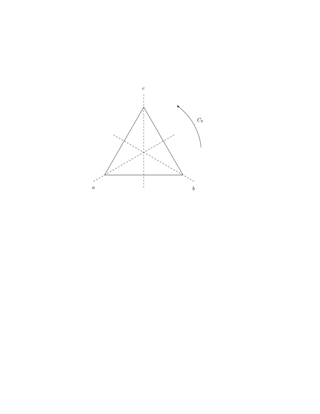
Figure 2: Symmetry axes of an equilateral triangle.

The number of classes in a finite group is equal to the number of nonequivalent irreducible representations of the group. One of the most interesting results of the theory of finite groups is the relation between the number of elements $g$ of a group and dimensions $n_{\nu}$ of its nonequivalent irreducible representations $\nu$,

$$\sum_{\nu}n_{\nu}^{2}\,=\,g.$$

Thus we find that the group $D_{3}$ has two nonequivalent one dimensional representations ${\bf 1_{A}}$, ${\bf 1_{B}}$ and one two dimensional representation ${\bf 2_{A}}$. Each representation is described by the set of characters  $\chi_{1},...,\chi_{\nu}$, where $\nu$ is the number of classes in the group. The character table for the group $D_{3}$ is given in Table 1.

$$\begin{array}[]{|c|c|c|c|}\hline\cr\quad D_{3}&\quad E&\quad C_{3}&\quad C_{a}\\ \hline\cr\hline\cr{\bf 1_{A}}&1&1&1\\ {\bf 1_{B}}&1&1&-1\\ {\bf 2_{A}}&2&-1&0\\ \hline\cr\end{array}$$

Table 1: The character table for the group $D_{3}$.

From the character table it is possible to find the decomposition of the product of any two representations:

$${\bf 1_{A}}\otimes{\bf 1_{A}}={\bf 1_{A}},\quad{\bf 1_{A}}\otimes{\bf 1_{B}}={\bf 1_{B}},\quad{\bf 1_{B}}\otimes{\bf 1_{B}}={\bf 1_{A}},$$ (39)

$${\bf 1_{A}}\otimes{\bf 2_{A}}={\bf 2_{A}},\quad{\bf 1_{B}}\otimes{\bf 2_{A}}={\bf 2_{A}},$$ (40)

$${\bf 2_{A}}\otimes{\bf 2_{A}}={\bf 1_{A}}\oplus{\bf 1_{B}}\oplus{\bf 2_{A}}.$$ (41)

To construct an explicit model obeying $D_{3}$ symmetry we need to specify the representation and determine invariant tensors. One dimensional representations coincide with the characters and the two dimensional representation can be chosen to be:

$$D(E)=\left(\begin{array}[]{cc}1&0\\ 0&1\end{array}\right)\;,\quad D(C_{3})=\left(\begin{array}[]{cc}\epsilon&0\\ 0&\epsilon^{-1}\end{array}\right)\;,\quad D(C_{a})=\left(\begin{array}[]{cc}0&1\\ 1&0\end{array}\right)\;,$$ (42)

where $\epsilon=e^{2\pi i/3}$.

Now it is straightforward to find the two singlets and the doublet in the decomposition of a product of two doublets (41). Writing $\psi=\{x,y\}$ and $\psi^{\prime}=\{x^{\prime},y^{\prime}\}$, we find:

$$\psi\otimes\psi^{\prime}\;|_{1_{A}}=xy^{\prime}+yx^{\prime}\;,$$ (43)

$$\psi\otimes\psi^{\prime}\;|_{1_{B}}=xy^{\prime}-yx^{\prime}\;,$$ (44)

$$\psi\otimes\psi^{\prime}\;|_{2}=\left(\begin{array}[]{c}yy^{\prime}\\ xx^{\prime}\\ \end{array}\right).$$ (45)

The decomposition (41) also reveals that the product of three doublets contains an invariant. Taking $\psi^{\prime\prime}=\{x^{\prime\prime},y^{\prime\prime}\}$, this invariant is:

$$\psi\otimes\psi^{\prime}\otimes\psi^{\prime\prime}\;|_{1_{A}}=xx^{\prime}x^{\prime\prime}+yy^{\prime}y^{\prime\prime}\;.$$ (46)

Finally, we want to show that given a doublet $\psi_{a}$ in $D_{3}$, there is a unique invariant norm given by $\psi_{a}^{*}\psi_{a}\equiv\psi_{1}^{*}\psi_{1}+\psi_{2}^{*}\psi_{2}$. Clearly, this norm is $D_{3}$ invariant since under a $D_{3}$ transformation $\psi_{a}^{\prime}=C_{ab}\psi_{b}$ with $C\subset D_{3}$ and $C^{\dagger}C=1$. That this is unique follows from the fact that in the product of two doublets there is a unique invariant given in eqn. (43). In addition, defining a new doublet by $\chi_{a}=g_{ab}\psi_{b}^{*}$ satisfying $\chi_{a}^{\prime}=C_{ab}\chi_{b}=(\psi_{b}^{*})^{\prime}g_{ba}^{T}=\psi_{c}^{*}C_{cb}^{\dagger}g_{ba}^{T}$ requires for consistency $g=CgC^{T}$. The unique solution to this consistency condition is $g=\left(\begin{array}[]{cc}0&1\\ 1&0\end{array}\right)$. Then we have $\chi\otimes\psi\;|_{1_{A}}\equiv\psi_{a}^{*}\psi_{a}$.

Appendix B. $D^{\prime}_{3}$ version of the model

The double group $D^{\prime}_{3}$ contains 12 elements in 6 classes. In addition to ${\bf 1_{A}}$, ${\bf 1_{B}}$, and ${\bf 2_{A}}$ representations which are already presented in $D_{3}$ it also has double-valued representations ${\bf 1_{C}}$, ${\bf 1_{\bar{C}}}$ and ${\bf 2_{B}}$. The character table of the double-valued representations is given in Table 2.

$$\begin{array}[]{|c|c|c|c|c|c|c|}\hline\cr\quad D_{3}&\quad E&\quad R&\quad C_{3}&\quad C_{3}R&\quad C_{a}&\quad C_{a}R\\ \hline\cr\hline\cr{\bf 1_{C}}&1&-1&-1&1&i&-i\\ {\bf 1_{\bar{C}}}&1&-1&-1&1&-i&i\\ {\bf 2_{B}}&2&-2&1&-1&0&0\\ \hline\cr\end{array}$$

Table 2: The character table for double-valued representations of the group $D^{\prime}_{3}$.

Multiplication rules are given in Table 3 and equations (41), (47) and (48).

$$\begin{array}[]{|c|c|c|c|c|c|c|}\hline\cr\quad D^{\prime}_{3}&\quad{\bf 1_{A}}&\quad{\bf 1_{B}}&\quad{\bf 1_{C}}&\quad{\bf 1_{\bar{C}}}&\quad{\bf 2_{A}}&{\bf 2_{B}}\\ \hline\cr\hline\cr{\bf 1_{A}}&{\bf 1_{A}}&{\bf 1_{B}}&{\bf 1_{C}}&{\bf 1_{\bar{C}}}&{\bf 2_{A}}&{\bf 2_{B}}\\ {\bf 1_{B}}&&{\bf 1_{A}}&{\bf 1_{\bar{C}}}&{\bf 1_{C}}&{\bf 2_{A}}&{\bf 2_{B}}\\ {\bf 1_{C}}&&&{\bf 1_{B}}&{\bf 1_{A}}&{\bf 2_{B}}&{\bf 2_{A}}\\ {\bf 1_{\bar{C}}}&&&&{\bf 1_{B}}&{\bf 2_{B}}&{\bf 2_{A}}\\ \hline\cr\end{array}$$

Table 3: Multiplication rules for the group $D^{\prime}_{3}$.

$${\bf 2_{A}}\otimes{\bf 2_{B}}={\bf 1_{C}}\oplus{\bf 1_{\bar{C}}}\oplus{\bf 2_{B}}\;,$$ (47)

$${\bf 2_{B}}\otimes{\bf 2_{B}}={\bf 1_{A}}\oplus{\bf 1_{B}}\oplus{\bf 2_{A}}\;.$$ (48)

The double-valued two dimensional representation can be chosen to be:

$$D(E)=\left(\begin{array}[]{cc}1&0\\ 0&1\end{array}\right)\;,\quad D(C_{3})=\left(\begin{array}[]{cc}\epsilon^{1/2}&0\\ 0&\epsilon^{-1/2}\end{array}\right)\;,\quad D(C_{a})=\left(\begin{array}[]{cc}0&1\\ -1&0\end{array}\right)\;,$$ (49)

and $D(R)=-D(E)$. As before, $\epsilon=e^{2\pi i/3}$.

Now it is straightforward to find new invariants. Taking the ${\bf 2_{A}}$ doublet $\psi=\{x,y\}$ and ${\bf 2_{B}}$ doublets $\varphi=\{a,b\}$, $\varphi^{\prime}=\{a^{\prime},b^{\prime}\}$ we find:

$$\varphi\otimes\varphi^{\prime}\;|_{1_{A}}\;=\;ab^{\prime}-ba^{\prime}\;,$$ (50)

$$\psi\otimes\varphi\otimes\varphi^{\prime}\;|_{1_{A}}\;=\;xbb^{\prime}+yaa^{\prime}\;.$$ (51)

With these results it is straightforward to check that the fermion masses and mixing angles we obtained in section 3 can be also obtained if we assume a $D^{\prime}_{3}\times U(1)$ family symmetry. In this case all doublets charged nontrivially under $SO(10)$ are in the ${\bf 2_{B}}$ of $D^{\prime}_{3}$, while singlets transform trivially under $D^{\prime}_{3}$. “Flavon” fields are in representations: $\phi_{a}={\bf 2_{A}}$, $\tilde{\phi}_{a}={\bf 2_{B}}$ and $A={\bf 1_{A}}$. “Flavon” doublets are expected to obtain vevs $\langle\phi_{a}\rangle=\phi\;\delta_{a1}$ and $\langle\tilde{\phi}_{a}\rangle=\tilde{\phi}\;\delta_{a1}$.

In the neutrino sector the doublets transform in the ${\bf 2_{B}}$ and the singlets transform trivially under $D^{\prime}_{3}$. Finally, the fields entering the superpotential for the “flavon” doublets transform in the following way: $\psi_{a}={\bf 2_{B}}$, $S={\bf 1_{C}}$, and $S_{\phi}={\bf 1_{\bar{C}}}$.

The advantage of $D^{\prime}_{3}$ (and $D^{\prime}_{N}$s in general) is that the ${\bf 2_{B}}$ representation of $D^{\prime}_{3}$ appears alone in the decomposition of a ${\bf 2}$ of $SU(2)$. Representations of $SU(2)$ decompose into irreducible representations of $D^{\prime}_{3}$ in the following way:

$${\bf 2} \rightarrow {\bf 2_{B}}\;,$$

$${\bf 3} \rightarrow {\bf 1_{B}}\;+\;{\bf 2_{A}}$$ (52)

$${\bf 4} \rightarrow {\bf 1_{C}}\;+\;{\bf 1_{\bar{C}}}\;+\;{\bf 2_{B}}\;,$$ (53)

$$\vdots$$

Because all doublets with nontrivial $SO(10)$ quantum numbers transform as ${\bf 2_{B}}$ under $D^{\prime}_{3}$ and all singlets with nontrivial $SO(10)$ quantum numbers are trivial singlets under $D^{\prime}_{3}$ the anomaly cancellation conditions are automatically satisfied. For the $SO(10)$ singlet with non-trivial $D^{\prime}_{3}$ quantum number, ($\phi_{a}$), at the least we must add an $SO(10)$ singlet transforming as a ${\bf 1_{B}}$.

Appendix C. Results for charged fermion masses, mixing angles and neutrino oscillations

In the paper [7] a global $\chi^{2}$ analysis has been performed incorporating two (one) loop renormalization group[RG] running of dimensionless (dimensionful) parameters from $M_{G}$ to $M_{Z}$ in the MSSM, one loop radiative threshold corrections at $M_{Z}$, and 3 loop QCD (1 loop QED) RG running below $M_{Z}$. Electroweak symmetry breaking is obtained self-consistently from the effective potential at one loop, with all one loop threshold corrections included. This analysis is performed using the code of Blažek et.al. [18].

In Table 4 we give the 20 observables which enter the $\chi^{2}$ function, their experimental values and the uncertainty $\sigma$ (in parentheses). These are the results for one set of soft SUSY breaking parameters $m_{0},\;M_{1/2}$ with all other parameters varied to obtain the best fit solution. In most cases $\sigma$ is determined by the 1 standard deviation experimental uncertainty, however in some cases the theoretical uncertainty ($\sim$ 0.1%) inherent in our renormalization group running and one loop threshold corrections dominates.

Table 4: Charged fermion masses and mixing angles
Initial parameters:
(1/$\alpha_{G},\,M_{G},\,\epsilon_{3}$) = ($24.52,\,3.05\cdot 10^{16}$ GeV,$\,-4.08$%),
($\lambda,\,$r$,\,\sigma,\,\epsilon,\,\rho,\,\epsilon^{\prime}$) = ($0.79,\,12.4,\,0.84,\,0.011,\,0.043,\,0.0031$),
($\Phi_{\sigma},\,\Phi_{\epsilon},\,\Phi_{\rho}$) = ($0.73,\,-1.21,\,3.72$)rad,
($m_{0},\,M_{1/2},\,A_{0},\,\mu(M_{Z})$) = ($1000,\,300,\,-1437,\,110$) GeV,
($(m_{H_{d}}/m_{0})^{2},\,(m_{H_{u}}/m_{0})^{2},\,$tan$\beta$) = ($2.22,\,1.65,\,53.7$).

$$\begin{array}[]{|l|c|l|}\hline\cr{\rm Observable}&{\rm Data}(\sigma)&Theory\\ \mbox{ }&{\rm(masses}&{\rm in\ \ GeV)}\\ \hline\cr\;\;\;M_{Z}&91.187\ (0.091)&91.17\\ \;\;\;M_{W}&80.388\ (0.080)&80.40\\ \;\;\;G_{\mu}\cdot 10^{5}&1.1664\ (0.0012)&1.166\\ \;\;\;\alpha_{EM}^{-1}&137.04\ (0.14)&137.0\\ \;\;\;\alpha_{s}(M_{Z})&0.1190\ (0.003)&0.1174\\ \;\;\;\rho_{new}\cdot 10^{3}&-1.20\ (1.3)&+0.320\\ \hline\cr\;\;\;M_{t}&173.8\ (5.0)&175.0\\ \;\;\;m_{b}(M_{b})&4.260\ (0.11)&4.328\\ \;\;\;M_{b}-M_{c}&3.400\ (0.2)&3.421\\ \;\;\;m_{s}&0.180\ (0.050)&0.148\\ \;\;\;m_{d}/m_{s}&0.050\ (0.015)&0.0589\\ \;\;\;Q^{-2}&0.00203\ (0.00020)&0.00201\\ \;\;\;M_{\tau}&1.777\ (0.0018)&1.776\\ \;\;\;M_{\mu}&0.10566\ (0.00011)&.1057\\ \;\;\;M_{e}\cdot 10^{3}&0.5110\ (0.00051)&0.5110\\ \;\;\;V_{us}&0.2205\ (0.0026)&0.2205\\ \;\;\;V_{cb}&0.03920\ (0.0030)&0.0403\\ \;\;\;V_{ub}/V_{cb}&0.0800\ (0.02)&0.0691\\ \;\;\;\hat{B}_{K}&0.860\ (0.08)&0.8703\\ \hline\cr{B(b\!\rightarrow\!s\gamma)\!\cdot\!10^{4}}&3.000\ (0.47)&2.995\\ \hline\cr\vrule\lx@intercol{\rm TOTAL}\;\;\;\;\chi^{2}\hfil\lx@intercol 3.39&\\ \hline\cr\end{array}$$

For large tan$\beta$ there are 6 real Yukawa parameters and 3 complex phases $\Phi_{\rho},\;\Phi_{\epsilon}$ and $\Phi_{\sigma}$. With 13 fermion mass observables (charged fermion masses and mixing angles [$\hat{B}_{K}$ replacing $\epsilon_{K}$ as a “measure of CP violation”]) we have 4 predictions. For low tan$\beta$ , $\lambda\neq\xi$, we have one less prediction. From Table 4 it is clear that this theory fits the low energy data quite well.

Finally, the squark, slepton, Higgs and gaugino spectrum of the theory is consistent with all available data. The lightest chargino and neutralino are higgsino-like with the masses close to their respective experimental limits. As an example of the additional predictions of this theory consider the CP violating mixing angles which may soon be observed at B factories. For the selected fit it was found

$$(\sin 2\alpha,\,\sin 2\beta,\,\sin\gamma)= (0.74,\,0.54,\,0.99)$$ (54)

or equivalently the Wolfenstein parameters

$$(\rho,\,\eta)= (-0.04,\,0.31)$$ . (55)

The results obtained in ref. [7] for the neutrino sector are presented in Tables  5 and  6. The model has maximal $\nu_{\mu}\rightarrow\nu_{\tau}$ mixing to describe atmospheric neutrino data and small mixing angle [SMA] $\nu_{e}\rightarrow\nu_{s}$ oscillations to fit solar neutrino data with SMA matter enhanced MSW oscillations. The model cannot however fit the LSND $\nu_{e}\rightarrow\nu_{\mu}$ data.

Table 5: Fit to atmospheric and solar neutrino
oscillations
Initial parameters: ( 4 neutrinos   with large tan$\beta$ )     $m^{\prime}=7.11\cdot 10^{-2}$ eV ,  $b$ = $-0.521$,  $c$ = 0.278, $\Phi_{b}$ = 3.40rad

$$\begin{array}[]{|c|c|}\hline\cr{\rm Observable}&{\rm Computed\;\;value}\\ \hline\cr\delta m^{2}_{atm}&3.2\cdot 10^{-3}\ \rm eV^{2}\\ \sin^{2}2\theta_{atm}&1.08\\ \delta m^{2}_{sol}&4.2\cdot 10^{-6}\ \rm eV^{2}\\ \sin^{2}2\theta_{sol}&3.0\cdot 10^{-3}\\ \hline\cr\end{array}$$

Table 6: Neutrino Masses and Mixings           
Mass eigenvalues [eV]:    0.0,  0.002,  0.04,  0.07          
Magnitude of neutrino mixing matrix U_αi                
$i=1,\cdots,4$ – labels mass eigenstates.              
$\alpha=\{e,\ \mu,\ \tau,\ s\}$ labels flavor eigenstates.

$$\left[\begin{array}[]{cccc}0.998&0.0204&0.0392&0.0529\\ 0.0689&0.291&0.567&0.767\\ 0.317\cdot 10^{-3}&0.145&0.771&0.620\\ 0.284\cdot 10^{-3}&0.946&0.287&0.154\\ \end{array}\right]$$

References

- [1] S. Dimopoulos and H. Georgi, Nucl. Phys. B193 (1981) 150; L.J. Hall, V.A. Kostelecky and S. Raby, Nucl. Phys. B267 (1986) 415; H. Georgi, Phys.Lett. 169B (1986) 231; F. Borzumati and A. Masiero, Phys. Rev. Lett. 57 (1986) 961; R. Barbieri and L.J. Hall, Phys. Lett. B338 (1994) 212; R. Barbieri, L.J. Hall and A. Strumia, Nucl. Phys. B445 (1995) 219; J. Hisano, T. Moroi, K. Tobe, M. Yamaguchi and T. Yanagida, Phys. Lett. B357 (1995) 579; F. Gabbiani, E. Gabrielli, A. Masiero and L. Silvestrini, Nucl. Phys. B477 (1996) 321; S. Dimopoulos and A. Pomarol, Phys. Lett. B353 (1995) 222; J. Hisano, T. Moroi, K. Tobe and M. Yamaguchi, Phys. Rev. D53 (1996) 2442; ibid., Phys. Lett. B391 (1997) 341; K. Tobe, Nucl. Phys. (Proc. Suppl.) B59 (1997) 223; J. Hisano, D. Nomura and T. Yanagida, Phys. Lett. B437 (1998) 351; J. Hisano, D. Nomura, Y. Okada, Y. Shimizu and M. Tanaka, Phys. Rev. D58 (1998) 116010; J. Hisano and D. Nomura, Phys. Rev. D59 (1999) 116005.
- [2] Y. Nir and N. Seiberg, Phys. Lett. B309 (1993) 337; P. Pouliot and N. Seiberg, Phys. Lett. B318 (1993) 169; M. Leurer, Y. Nir and N. Seiberg, Nucl. Phys. B398 (1993) 319; M. Leurer, Y. Nir and N. Seiberg, Nucl. Phys. B420 (1994) 468;
- [3] E. Dudas, S. Pokorski and C.A. Savoy, Phys. Lett. B356 (1995) 45; and ibid., Phys. Lett. B369 (1996) 255; P. Binetruy, S. Lavignac and P. Ramond, Nucl. Phys. B477 (1996) 353; A.E. Faraggi and J.C. Pati, Nucl. Phys. B526 (1998) 21.
- [4] D. Kaplan and M. Schmaltz, Phys. Rev. D49 (1994) 3741; Z. Berezhiani, Phys.Lett. B417 (1998) 287.
- [5] M. Dine, R. Leigh and A. Kagan, Phys. Rev. D48 (1993) 4269; A. Pomarol and D. Tommasini, Nucl.Phys. B466 (1996) 3; R. Barbieri, G. Dvali and L.J. Hall, Phys. Lett. B377 (1996) 76; R. Barbieri and L.J. Hall, Nuovo Cim. 110A (1997) 1.
- [6] R. Barbieri, L.J. Hall, S. Raby and A. Romanino, Nucl. Phys. B493 (1997) 3; R. Barbieri, L.J. Hall and A. Romanino, Phys. Lett. B401 (1997) 47.
- [7] T. Blažek, S. Raby and K. Tobe, accepted for publication in Phys. Rev. D (1999), hep-ph/9903340.
- [8] P.H. Frampton and T.W. Kephart, Phys. Rev. D51 (1995) 1; and ibid., Int. J. Mod. Phys. A10 (1995) 4689; L.J. Hall and H. Murayama, Phys. Rev. Lett. 75 (1995) 3985; P.H. Frampton and O.C.W. Kong, Phys. Rev. Lett. 77 (1996) 1699; C.D. Carone and R.F. Lebed, Phys. Rev. D60 (1999) 096002; P.H. Frampton and A. Rašin, hep-ph/9910522.
- [9] A. Aranda, C. D. Carone and R. F. Lebed, hep-ph/9910392.
- [10] S. Giddings and A. Strominger, Nucl. Phys. B307 (1988) 854; S. Coleman, Nucl. Phys. B310 (1988) 643; G. Gilbert, Nucl. Phys. B328 (1989) 159.
- [11] Y. Kawamura, H. Murayama and M. Yamaguchi, Phys. Rev. D51 (1995) 1337; K.S. Babu and R.N. Mohapatra, Phys. Rev. Lett. 83 (1999), 2522.
- [12] L. Krauss and F. Wilczek, Phys. Rev. Lett. 62 (1989) 1221.
- [13] M. Hamermesh, Group Theory and Its Application to Physical Problems, Addison-Wesley, 1962; A. D. Thomas and G. V. Wood, Group tables, Shiva publishing, 1980.
- [14] A. Mafi, private communication and also R. Barbieri, L. Giusti, L.J. Hall and A. Romanino, Nucl. Phys. B550 (1999) 32.
- [15] T. Blažek, S. Raby and K. Tobe, paper in preparation.
- [16] M. Green and J. Schwarz, Phys. Lett. B149 (1984) 117; M. Dine, N. Seiberg and E. Witten, Nucl. Phys. B289 (1987) 589.
- [17] C. Froggatt and H.B. Nielsen, Nucl. Phys. B147 (1979) 277.
- [18] T. Blažek, M. Carena, S. Raby and C. Wagner, Phys. Rev. D56 (1997) 6919.
- [19] M. Gell-Mann, P. Ramond and R. Slansky, in Supergravity, ed. P. van Nieuwenhuizen and D.Z. Freedman, North-Holland, Amsterdam, 1979, p. 315; T. Yanagida, in Proceedings of the Workshop on the unified theory and the baryon number of the universe, ed. O. Sawada and A. Sugamoto, KEK report No. 79-18, Tsukuba, Japan, 1979.
- [20] G. Giudice and A. Masiero, Phys. Lett. B206 (1988) 480; J.E. Kim and H.P. Nilles, Mod. Phys. Lett. A9 (1994) 3575.
- [21] R.N. Mohapatra and J.W.F. Valle, Phys. Rev. D34 (1986) 1634.