IEM-FT-198/99 IFT-UAM/CSIC-99-42 CERN-TH/99-332 Electroweak and Flavor Physics in Extensions of the Standard Model with Large Extra Dimensions 

Abstract

We study the implications of extra dimensions of size $R\sim 1/$TeV on electroweak and flavor physics due to the presence of Kaluza-Klein excitations of the SM gauge-bosons. We consider several scenarios with the SM fermions either living in the bulk or being localized at different points of an extra dimension. Global fits to electroweak observables provide lower bounds on $1/R$, which are generically in the $2$–$5$ TeV range. We find, however, certain models where the fit to electroweak observables is better than in the SM, because of an improvement in the prediction to the weak charge $Q_{W}$. We also consider the case of softly-broken supersymmetric theories and we find new non-decoupling effects that put new constraints on $1/R$. If quarks of different families live in different points of the extra dimension, we find that the Kaluza-Klein modes of the SM gluons generate (at tree level) dangerous flavor and CP-violating interactions. The lower bounds on $1/R$ can increase in this case up to $5000$ TeV, disfavoring these scenarios in the context of TeV-strings.

1 Introduction

The existence of extra dimensions seems to be a crucial ingredient in the unification of gravity with the gauge forces. This is the case, for example, of string theory, where more than three spatial dimensions seem to be necessary for the consistency of the theory. It has often been assumed that these extra dimensions are compact, with radii of Planckean size, $R\sim 10^{-33}$ cm, and therefore irrelevant for phenomenological purposes.

Nevertheless, it has recently been suggested that these extra dimensions could, in fact, be very large and testable in present-day experiments. The first possibility of lowering the compactification scale to $\sim$TeV was given in Ref. [1]. A different, and more drastic, possibility, suggested in Refs. [2, 3], is to lower the fundamental (string) scale down to the electroweak scale. This scenario requires either very large extra dimensions, in which only gravity propagates [3], or a very small string coupling [4]. Having the fundamental (string) scale close to the TeV implies that the extra dimensions must appear at energies $\sim$ TeV (or below for the case of gravity), and therefore such a possibility can be tested in future colliders.

In this paper we want to study the implications of an extra TeV^-1 dimension. We will consider the case of the Standard Model (SM) gauge bosons propagating in this extra dimension, and analyze the implications of their Kaluza-Klein (KK) excitations for electroweak and flavor processes. The effects of these KK excitations are of two kinds. First, the KK excitations can mix with the $Z$ and $W$ boson of the SM and, consequently, modify their masses and couplings. Second, the KK excitations can induce new four-fermion operators in the SM lagrangian. All these effects are in principle large, since they arise at the tree level. Using the fact that the experimental data seem to be in excellent agreement with the SM, we will be able to put bounds on the compactification scale $M_{c}$. From the high-precision electroweak data, we obtain $M_{c}\gtrsim 2$–$5$ TeV (depending on the model). Since only the weak charge, $Q_{W}$, measured in atomic parity violation experiments, seems to depart by a few sigmas from the SM prediction [5, 6], we will briefly discuss how an extra dimension can improve the SM fit. KK excitations can also induce flavor-violating interactions if fermions of different families live at different points of the extra dimension, or if some of them are localized at fixed points and others live in the bulk of the extra dimension. We find that this possibility suffers from severe bounds on $M_{c}$, which are in certain cases as large as $M_{c}\gtrsim 5000$ TeV.

Part of the analysis done here has previously been considered in the literature [7, 8, 9, 10]. Our analysis, however, aims to be the most general one and thus it incorporates new scenarios not considered before. For example, we will allow some of the SM fermions to live in the bulk of the extra dimension, or to be localized at different points of the extra dimension. As we will see, these possibilities offer a new and rich phenomenology, especially concerning flavor physics. We will also consider the case in which the higher dimensional theory is supersymmetric and yields, after compactification to 4D, the minimal supersymmetric extension of the SM (MSSM). This case had not been analyzed before and we will show that, surprisingly, there are tree-level effects arising from integrating out the superpartners. The reason of these effects is the existence of a scalar SU(2)_L-triplet (required by supersymmetry in five dimensions) that gets a vacuum expectation value (VEV) of the order of $m^{2}_{W}/M_{c}$, and modifies the relation between the $Z$ and $W$ masses.

The outline of this paper is as follows. In section 2 we consider the SM in 5D and compute the effective 4D theory obtained after integrating out the KK excitations of the SM gauge fields, assuming the most general framework where the SM fermions can live either at fixed points or in the bulk of the extra dimension. In section 3 we perform a similar exercise for the case where the 5D theory is supersymmetric. We pay particular attention to the modification of the effective theory generated by the VEV of the 5D gauge superpartner. This VEV is always non-zero whenever a Higgs field acquires a VEV at the boundary of the extra dimension. In section 4 we compute the predictions of the theory for different electroweak observables, and present the corresponding bounds on $M_{c}$ in section 5. In section 6 we consider the effect of the KK excitation on flavor observables such as $\Delta m_{K}$, $\varepsilon_{K}$ and $\varepsilon^{\prime}_{K}$, and derive new bounds on $M_{c}$. Section 7 is devoted to our conclusions.

A word of caution on our calculation is in order. Since we are working with gauge theories in more than four dimensions, one could be worried about the validity of the perturbative expansion of the theory. Higher dimensional theories are known to be strongly coupled at energies above the compactification scale $M_{c}$, implying a cutoff at $\sim 10$–$100$ $M_{c}$. This means that we can only trust the effect of the first $10$–$100$ KK excitations. The effect of the heavy $n$ KK modes ($n>10$–$100$), although not calculable, is estimated to be $\lesssim 10\%$ of the light KK-modes effect. The uncertainty of the effect of an extra dimension in low-energy processes, $p\sim M_{Z}<M_{c}$, is thus lower than $10^{-1}\,M^{2}_{Z}/M_{c}^{2}\sim 10^{-3}\,({\rm TeV}/M_{c})^{2}$. Similarly stringy effects will be small if the string scale is at least one order of magnitude larger than the compactification radius as we will consider here.

2 The five-dimensional SM

The model we want to study is based on a simple extension of the SM to 5D [11]. The fifth dimension $x_{5}$ is compactified on the orbifold $S^{1}/\mathbb{Z}_{2}$, a circle of radius $R$ with the identification $x_{5}\rightarrow-x_{5}$. This is a segment of length $\pi R$ with two 4D boundaries, one at $x_{5}=0$ and another at $x_{5}=\pi R$ (the two fixed points of the orbifold). This type of compactification is needed to get chiral fermions. The SM gauge fields live in the 5D bulk, while the SM fermions, $\psi$, and the Higgs doublets, $H_{i}\ (i=1,2)$ , can either live in the bulk or be localized on the 4D boundaries. In this section we will assume that all the localized fields live on the $x_{5}=0$ boundary. We leave to section 6 the possibility to have localized fields living in different points of the extra dimension.

The 5D lagrangian is given by

$${\cal L}_{5D} = -\frac{1}{4g^{2}_{5}}F_{MN}^{2}+\sum_{i}\Big{[}(1-\varepsilon^{H_{i}})|D_{M}H_{i}|^{2}+(1-\varepsilon^{\psi_{i}})i\bar{\psi}_{i}\Gamma^{M}D_{M}\psi_{i}\Big{]}$$ (2.1)

$$+ \sum_{i}\Big{[}\varepsilon^{H_{i}}|D_{\mu}H_{i}|^{2}+\varepsilon^{\psi_{i}}i\bar{\psi}_{i}\sigma^{\mu}D_{\mu}\psi_{i}\Big{]}\delta(x_{5})\,,$$

where we have introduced the operator $\varepsilon$ defined as $\varepsilon^{F}=1\ (0)$ for the $F$-field living in the boundary (bulk); $D_{M}=\partial_{M}+iV_{M}$, $M=(\mu,5)$, and $g_{5}$ is the 5D gauge coupling. The fields living in the bulk can be defined to be even or odd under the $\mathbb{Z}_{2}$-parity, i.e. $\Phi_{\pm}(x_{5})=\pm\Phi_{\pm}(-x_{5})$. They can be Fourier-expanded as

$$\Phi_{+}(x_{\mu},x_{5}) = \sum^{\infty}_{n=0}\cos\frac{nx_{5}}{R}\Phi^{(n)}_{+}(x_{\mu})\,,$$

$$\Phi_{-}(x_{\mu},x_{5}) = \sum^{\infty}_{n=1}\sin\frac{nx_{5}}{R}\Phi^{(n)}_{-}(x_{\mu})\,,$$ (2.2)

where $\Phi^{(n)}_{\pm}$ are the KK excitations of the 5D fields. Gauge and Higgs bosons living in the 5D bulk will be assumed to be even under the $\mathbb{Z}_{2}$. Their (massless) zero modes will correspond to the gauge and Higgs SM fields. Fermions in 5D have two chiralities, $\psi_{L}$ and $\psi_{R}$, that can transform as even or odd under the $\mathbb{Z}_{2}$. The precise assignment is a matter of definition. We will choose the even assignment for the $\psi_{L}$ ($\psi_{R}$) components of fermions $\psi$, which are doublets (singlets) under SU(2)_L. As a consequence only the $\psi_{L}$ of SU(2)_L doublets and $\psi_{R}$ of SU(2)_L singlets have zero modes (see Eq. (2.2)) and the massless fermion sector is chiral.

Using Eq. (2.2) and integrating over the fifth dimension, we can easily obtain the theory in 4D. This will contain the SM fields plus their KK excitations. In order to study the impact of this theory in the electroweak and flavor processes, we will integrate out the KK excitations at the tree level and at the first order in the expansion parameter $X$ defined as 

$$X=\sum_{n=1}^{\infty}\frac{2}{n^{2}}\,\frac{m_{Z}^{2}}{M_{c}^{2}}=\frac{\pi^{2}}{3}\frac{m_{Z}^{2}}{M_{c}^{2}}\,,$$ (2.3)

where $M_{c}\equiv 1/R$. As we will see, this approximation is good enough since $X$ will be constrained to be very small.

To obtain the effective 4D theory, we only need to take into consideration the couplings of the SM fermions to the KK excitations of the electroweak gauge bosons and the mass terms of these latter. Notice that Higgses living on the boundary will induce mixing terms between the SM gauge bosons and their KK excitations (this is due to the breaking of $x_{5}$-translational invariance of the boundaries). We therefore define for later use the effective mixing angle 

$$s^{2}_{\alpha}=\varepsilon^{H_{2}}\,s^{2}_{\beta}+\varepsilon^{H_{1}}\,c^{2}_{\beta}\,,$$ (2.4)

where, as usual, we have introduced the mixing angle $\beta$ defined as $\tan\beta=\langle H_{2}\rangle/\langle H_{1}\rangle$, with $v^{2}\equiv\langle H_{1}\rangle^{2}+\langle H_{2}\rangle^{2}$ and $v\simeq 174$ GeV.

The charged electroweak sector

In the charged sector the 4D lagrangian can be written as 

$$\mathcal{L}^{ch}=\sum_{a=1}^{2}\mathcal{L}_{a}^{ch}$$ (2.5)

with

$$\mathcal{L}_{a}^{ch} = \frac{1}{2}m^{2}_{W}\left\{W_{a}\cdot W_{a}+2\sqrt{2}s^{2}_{\alpha}\sum_{n=1}^{\infty}W_{a}\cdot W_{a}^{(n)}\right\}+\frac{1}{2}M_{c}^{2}\sum_{n=1}^{\infty}\,n^{2}\,W_{a}^{(n)}\cdot W_{a}^{(n)}$$ (2.6)

$$- g\,W_{a}\cdot J_{a}-g\,\sqrt{2}J^{KK}_{a}\cdot\sum_{n=1}^{\infty}W_{a}^{(n)}\,,$$

where $m^{2}_{W}=g^{2}v^{2}/2$, the weak angle $\theta$ is defined by $e=g\,s_{\theta}=g^{\prime}\,c_{\theta}$, while the currents are

$$J_{a\mu} = \sum_{\psi}\bar{\psi}_{L}\gamma_{\mu}\frac{\sigma_{a}}{2}\psi_{L}\,,$$

$$J_{a\mu}^{KK} = \sum_{\psi}\varepsilon^{\psi_{L}}\bar{\psi}_{L}\gamma_{\mu}\frac{\sigma_{a}}{2}\psi_{L}\,.$$ (2.7)

For momenta $p^{2}\sim m_{W}^{2}\ll M_{c}^{2}$ we can integrate out the KK modes $W_{a}^{(n)}$ using their equations of motion and neglecting their kinetic terms. They yield

$$W_{a}^{(n)}=\frac{\sqrt{2}}{n^{2}\,M_{c}^{2}}\left[-s^{2}_{\alpha}m_{W}^{2}\,W_{a}+g\,J_{a}^{KK}\right]+\mathcal{O}(X^{2})\,.$$ (2.8)

Replacing the solution (2.8) into (2.6), we obtain

$$\mathcal{L}^{ch}_{a,\,eff}=\frac{1}{2}M^{2}_{W}W_{a}\cdot W_{a}-gW_{a}\cdot\left[J_{a}-s^{2}_{\alpha}\,c_{\theta}^{2}\,X\,J_{a}^{KK}\right]-\frac{g^{2}}{2\,m_{Z}^{2}}\,X\,J_{a}^{KK}\cdot J_{a}^{KK}\,,$$ (2.9)

where

$$M_{W}^{2}=\left[1-s^{4}_{\alpha}c^{2}_{\theta}X\right]\,m_{W}^{2}\,.$$ (2.10)

Finally, for very low momenta, much smaller than the weak scale $p^{2}\ll M_{W}^{2}$, the $W_{a}$ gauge bosons can also be integrated out from the lagrangian (2.9). The result can be written as

$$\mathcal{L}^{ch}_{a,\,low}=-\frac{g^{2}}{2M_{W}^{2}}\left\{\left[J_{a}-s^{2}_{\alpha}\,c_{\theta}^{2}\,X\,J_{a}^{KK}\right]^{2}+\,c_{\theta}^{2}\,X\,J_{a}^{KK}\cdot J_{a}^{KK}\right\}\,.$$ (2.11)

We can use the lagrangian (2.11) to describe the $\mu$ decay, from where the Fermi constant is found to be

$$\frac{G_{F}}{\sqrt{2}}=\frac{g^{2}}{8M_{W}^{2}}\Big{[}1+\{\varepsilon^{\ell_{1\,L}}\varepsilon^{\ell_{2\,L}}-(\varepsilon^{\ell_{1\,L}}+\varepsilon^{\ell_{2\,L}})s^{2}_{\alpha}\}c^{2}_{\theta}X\Big{]}\,.$$ (2.12)

If we assume that the KK modes do not spoil lepton universality (as we will do in this section), Eq. (2.12) can be written as

$$\frac{G_{F}}{\sqrt{2}}=\frac{g^{2}}{8M_{W}^{2}}\left[1+\varepsilon^{\ell_{L}}c_{2\alpha}c^{2}_{\theta}X\right]\,.$$ (2.13)

The neutral sector

In the neutral sector the 4D lagrangian can be similarly written as

$$\mathcal{L}^{neutral} = \frac{1}{2}m_{Z}^{2}\,\left\{Z\cdot Z+2\sqrt{2}s^{2}_{\alpha}\sum_{n=1}^{\infty}Z\cdot Z^{(n)}\right\}+\frac{1}{2}M_{c}^{2}\sum_{n=1}^{\infty}n^{2}\,\left[Z^{(n)}\cdot Z^{(n)}+A^{(n)}\cdot A^{(n)}\right]$$ (2.14)

$$- \frac{e}{s_{\theta}c_{\theta}}\left[Z\cdot J_{Z}+\sqrt{2}\sum_{n=1}^{\infty}Z^{(n)}\cdot J_{Z}^{KK}\right]-e\left[A\cdot J_{em}+\sqrt{2}\sum_{n=1}^{\infty}A^{(n)}\cdot J_{em}^{KK}\right]\,,$$

where $m^{2}_{Z}=(g^{2}+g^{\prime\,2})v^{2}/2$ and the currents are

$$J_{\mu\,Z} = \sum_{\psi}\bar{\psi}\,\gamma_{\mu}\left(g_{V}^{\psi}+\gamma_{5}\,g_{A}^{\psi}\right)\psi\,,$$

$$J_{\mu\,Z}^{KK} = \sum_{\psi}\bar{\psi}\,\gamma_{\mu}\left(g_{V}^{\psi,KK}+\gamma_{5}\,g_{A}^{\psi,KK}\right)\psi\,,$$

$$J_{\mu\,em}^{KK} = \sum_{\psi}\bar{\psi}\,\gamma_{\mu}\left(g_{em,V}^{\psi,KK}+\gamma_{5}\,g_{em,A}^{\psi,KK}\right)\psi\,.$$ (2.15)

The vector and axial couplings are defined by

$$g_{V}^{\psi} = \frac{T_{3}}{2}-s^{2}_{\theta}\ Q\,,$$

$$g_{A}^{\psi} = -\frac{T_{3}}{2}\,,$$

$$g_{V}^{\psi,\,KK} = \varepsilon^{\psi_{L}}\left(\frac{T_{3}}{2}-s^{2}_{\theta}\,\frac{Q}{2}\right)-\varepsilon^{\psi_{R}}s^{2}_{\theta}\,\frac{Q}{2}\,,$$

$$g_{A}^{\psi,\,KK} = \varepsilon^{\psi_{L}}\left(-\frac{T_{3}}{2}+s^{2}_{\theta}\,\frac{Q}{2}\right)-\varepsilon^{\psi_{R}}s^{2}_{\theta}\,\frac{Q}{2}\,,$$

$$g_{em,\,V}^{\psi,\,KK} = \left(\varepsilon^{\psi_{R}}+\varepsilon^{\psi_{L}}\right)\,\frac{Q}{2}\,,$$

$$g_{em,\,A}^{\psi,\,KK} = \left(\varepsilon^{\psi_{R}}-\varepsilon^{\psi_{L}}\right)\,\frac{Q}{2}\,.$$ (2.16)

For momenta $p^{2}\ll M^{2}_{c}$ the $Z^{(n)}$ and $A^{(n)}$ modes can be integrated out, yielding the effective lagrangian

$$\mathcal{L}^{neutral}_{eff} = \frac{1}{2}M_{Z}^{2}\,Z\cdot Z-\frac{e}{s_{\theta}\,c_{\theta}}\,Z\cdot\left[J_{Z}-\,s^{2}_{\alpha}X\,J_{Z}^{KK}\right]-eA\cdot J_{em}$$ (2.17)

$$- \frac{1}{2\,M_{Z}^{2}}\,\frac{e^{2}}{s^{2}_{\theta}\,c^{2}_{\theta}}\,XJ_{Z}^{KK}\cdot J_{Z}^{KK}-\frac{e^{2}}{2\,M_{Z}^{2}}\,X\,J_{em}^{KK}\cdot J_{em}^{KK}\,,$$

where we have defined

$$M_{Z}^{2}=\left[1-s^{4}_{\alpha}X\right]m_{Z}^{2}\,.$$ (2.18)

For momenta $p^{2}\ll M_{Z}^{2}$ we can integrate out the SM $Z$-boson and obtain the neutral lagrangian

$$\mathcal{L}^{neutral}_{low} = -\,\frac{1}{2M_{Z}^{2}}\,\frac{e^{2}}{s^{2}_{\theta}\,c^{2}_{\theta}}\,\left\{\left[J_{Z}-s^{2}_{\alpha}X\,J_{Z}^{KK}\right]^{2}-\,X\,J_{Z}^{KK}\cdot J_{Z}^{KK}\right\}$$ (2.19)

$$- eA\cdot J^{em}-\frac{e^{2}}{2\,M_{Z}^{2}}X\,J_{em}^{KK}\cdot J_{em}^{KK}\,.$$

Using now Eqs. (2.10), (2.13) and (2.18) one can relate the angle $\theta$ to the Fermi constant as

$$s^{2}_{\theta}\,c^{2}_{\theta}=\frac{\pi\alpha}{\sqrt{2}\,G_{F}\,M_{Z}^{2}}\,\left(1+\Delta\right)\,,$$ (2.20)

where

$$\Delta=\left[\varepsilon^{\ell_{L}}c_{2\alpha}c^{2}_{\theta}-s^{4}_{\alpha}s^{2}_{\theta}\right]\,X\,,$$ (2.21)

and the effective lagrangian can be cast as

$$\mathcal{L}^{neutral}_{low} = -\,4\,\frac{G_{F}}{\sqrt{2}}\,(1-\Delta)\left\{\left[J_{Z}-s^{2}_{\alpha}X\,J_{Z}^{KK}\right]^{2}-\,X\,J_{Z}^{KK}\cdot J_{Z}^{KK}\right\}$$ (2.22)

$$- eA\cdot J^{em}-\frac{2\pi\alpha}{M_{Z}^{2}}X\,J_{em}^{KK}\cdot J_{em}^{KK}\,.$$

3 The five-dimensional supersymmetric case

If the theory in 5D is supersymmetric, the field content must be extended to complete $N=2$ supermultiplets [12, 11]. The on-shell field content of the gauge supermultiplet is $\mathbb{V}=(V_{\mu},V_{5},\lambda^{i},\Sigma)$ where $\lambda^{i}\ (i=1,2)$ is a simplectic Majorana spinor and $\Sigma$ a real scalar in the adjoint representation; $(V_{\mu},\lambda^{1})$ is even under $\mathbb{Z}_{2}$ and $(V_{5},\Sigma,\lambda^{2})$ is odd. Matter and Higgs fields are arranged in $N=2$ hypermultiplets that consist of chiral and antichiral $N=1$ supermultiplets. The chiral $N=1$ supermultiplets are even under $\mathbb{Z}_{2}$ and contain massless states. These will correspond to the SM fermions and Higgs. Because of anomaly cancellation, the Higgs doublet fields must come in pairs, $H_{1}$ and $H_{2}$. For simplicity we will just consider one pair of Higgs doublets.

Supersymmetry must be broken to give masses to all the superpartners. We will not specify the way supersymmetry is broken, but assume that the superpartner masses are of order $M_{c}$. For a specific example see Ref. [11]. A priori one would think that integrating out the superpartners at tree level does not lead to any effect in the SM lagrangian, as is the case for the 4D supersymmetric extension of the SM. Nevertheless, this is not true for the 5D supersymmetric case. As we will show below, integrating out the scalar field $\Sigma$ induces a tree-level contribution to the SM lagrangian.

The 5D lagrangian for the scalar $\Sigma$ can be written as

$$\mathcal{L}_{5D,\Sigma}={\rm Tr}\,\frac{1}{g_{5}^{2}}\,\left|D_{\mu}\Sigma\right|^{2}+{\rm Tr}\,\frac{1}{g_{5}^{2}}\,\left|D_{5}\Sigma\right|^{2}-\sum_{i=1}^{2}(1-\varepsilon^{H_{i}})H_{i}^{\dagger}\Sigma^{2}H_{i}$$

$$-\left[\sum_{i=1}^{2}\varepsilon^{H_{i}}H_{i}^{\dagger}(\partial_{5}\Sigma)H_{i}+\frac{g_{5}^{2}}{2}\sum_{\alpha}\left(\sum_{i=1}^{2}\varepsilon^{H_{i}}H_{i}^{\dagger}T^{\alpha}H_{i}\right)^{2}\delta(x_{5})\right]\delta(x_{5})\,,$$ (3.1)

where only the bosonic interactions of $\Sigma$ with the Higgs have been considered. Using the fact that $\Sigma$ is odd under $\mathbb{Z}_{2}$-parity and integrating over $x_{5}$, we can obtain from Eq. (3) a potential for the KK modes of $\Sigma$. Due to the linear term in $\Sigma$ in Eq. (3), the VEV of $H_{i}$ on the boundary induces a VEV for the KK modes of $\Sigma$. Since the field $\Sigma$ transforms under SU(2)${}_{L}\times$U(1)_Y as $(\mathbf{3},0)+(\mathbf{1},0)$, its triplet-component VEV will give a mass to the $W$ gauge boson, while its singlet-component does not couple to anything and is harmless. Let us see this explicitly. The triplet component of $\Sigma$ can be written, in matrix notation, as

$$\Sigma=\left(\begin{array}[]{cc}\xi_{0}/2&\xi^{+}/\sqrt{2}\\ &\\ \xi^{-}/\sqrt{2}&-\xi_{0}/2\\ \end{array}\right)\,.$$ (3.2)

Upon integration over $x_{5}$ and putting the Higgs fields $H_{i}$ at their VEVs, we obtain the potential for the KK modes of $\xi_{0}$

$$V_{\,\Sigma}=\frac{M_{c}^{2}}{2}\ \sum_{n=1}^{\infty}\left\{n\,\xi_{0}^{(n)}-\frac{g}{\sqrt{2}}\,\left(\varepsilon^{H_{2}}s_{\beta}^{2}-\varepsilon^{H_{1}}c_{\beta}^{2}\right)\,\frac{v^{2}}{M_{c}}\right\}^{2}+\frac{g^{2}}{8}\,c_{2\beta}^{2}\,v^{4}\ .$$ (3.3)

Equation (3.3) yields a VEV for $\xi_{0}^{(n)}$, which is given by

$$\langle\xi_{0}^{(n)}\rangle=\frac{1}{n}\,\left(\varepsilon^{H_{2}}s_{\beta}^{2}-\varepsilon^{H_{1}}c_{\beta}^{2}\right)\,\frac{m_{W}}{M_{c}}\,v\,.$$ (3.4)

Since these VEVs induce a mass term for the $W$, Eq. (2.10) must be corrected in the supersymmetric case to

$$M_{W}^{2}=\left[1-\varepsilon^{H_{1}}\varepsilon^{H_{2}}\,s_{2\beta}^{2}\,c^{2}_{\theta}X\right]\,m_{W}^{2}\,.$$ (3.5)

Notice that the two terms, the one in Eq. (2.10) proportional to $-s^{4}_{\alpha}=-(\varepsilon^{H_{2}}s_{\beta}^{2}+\varepsilon^{H_{1}}c_{\beta}^{2})^{2}$ and the other proportional to $(\varepsilon^{H_{2}}s_{\beta}^{2}-\varepsilon^{H_{1}}c_{\beta}^{2})^{2}$ from the triplet, combine into an effective term proportional to $\varepsilon^{H_{1}}\varepsilon^{H_{2}}\,s_{2\beta}^{2}$. This cancels in all cases, except if both Higgs doublets live on the boundary. Because of the change in $M^{2}_{W}$, $\Delta$ defined in Eq. (2.21) must be replaced by

$$\Delta=\left[\varepsilon^{\ell_{L}}c_{2\alpha}\,c^{2}_{\theta}-s^{4}_{\alpha}+\varepsilon^{H_{1}}\varepsilon^{H_{2}}\,s^{2}_{2\beta}\,c^{2}_{\theta}\right]\,X\,.$$ (3.6)

Therefore we conclude that for the 5D supersymmetric case we obtain the same low-energy lagrangian as for the non-supersymmetric case, with the replacement of Eqs. (2.10) and (2.21) by Eqs. (3.5) and (3.6), respectively.

4 Electroweak observables

The physical observables in the Standard Model can be predicted as functions of some input parameters. One usually chooses as input parameters the best measured ones, i.e. the Fermi constant $G_{F}=1.166\times 10^{-5}$ GeV^-2, the fine-structure constant $\alpha=1/137.036$ (or $\alpha(M_{Z})=1/128.933$) and the mass of the $Z$ gauge-boson $M_{Z}=91.1871$ GeV. To make a reliable prediction of the other observables, one has to include Standard Model radiative corrections as well as corrections due to the presence of KK modes. In section 2 we have only included tree-level physics. This is correct for the KK modes since their masses will be constrained to be large. We will neglect electroweak radiative corrections to $\mathcal{O}(X)$ effective operators, because their contribution is inside the rest of uncertainties in the calculation, in particular those coming from the contribution of heavy ($n\gtrsim 10$) KK modes, as was pointed out in section 1. For practical purposes we use, in the couplings of the KK modes, Eq. (2), the weak angle [13] $s^{2}_{\theta}\equiv s^{2}_{M_{Z}}\simeq 0.231$.

The set of physical observables we have chosen for our fit is given in Table 1, where the experimental values and Standard Model predictions used in the fit are collected from Ref. [13].

Observable	Experimental value	Standard Model prediction
$M_{W}$ (GeV)	80.394$\pm$0.042	80.377$\pm$0.023 ($-$0.036)
$\Gamma_{\ell\ell}$ (MeV)	83.958$\pm$0.089	84.00$\pm$0.03 ($-$0.04)
$\Gamma_{had}$ (GeV)	1.7439$\pm$0.0020	1.7433$\pm$0.0016 ($-$0.0005)
$A_{FB}^{\ell}$	0.01701$\pm$0.00095	0.0162$\pm$0.0003 ($-0.0004$)
$Q_{W}$	$-$72.06$\pm$0.46	$-$73.12$\pm$0.06 ($+$0.01)
$\sum_{i=1}^{3}\left|V_{1i}\right|^{2}$	0.9969$\pm$0.0022	1 (unitarity)

Table 1: Set of physical observables

The Standard Model predictions correspond to a Higgs mass $M_{H}=M_{Z}$ and a top-quark mass $m_{t}=173\pm 4$ GeV. The global shift in the prediction when $M_{H}$ is shifted to 300 GeV is shown in parenthesis. The observables in Table 1 can be classified into LEP (high-energy) and low-energy observables.

LEP observables

The formalism we have developed in sections 2 and 3 allows us to write the prediction for these observables in terms of the Standard Model predictions. In particular one can compute the prediction for $M_{W}$ as

$$M_{W}^{2}=\left(M_{W}^{2}\right)^{SM}\left[1-\frac{s^{2}_{\theta}}{c_{2\theta}}\Delta+\Delta_{W}\,\right]\,,$$ (4.1)

where, for the non-supersymmetric case,

$$\Delta_{W}=s^{2}_{\theta}\,s^{4}_{\alpha}\,X\,,$$ (4.2)

whereas for the supersymmetric case

$$\Delta_{W}=\left[s^{2}_{\theta}\,s^{4}_{\alpha}+c^{2}_{\theta}\left(\varepsilon^{H_{2}}s^{2}_{\beta}\,-\varepsilon^{H_{1}}c^{2}_{\beta}\right)\right]\,X\ .$$ (4.3)

We indicate with the $SM$ superindex the Standard Model prediction including radiative corrections.

The rest of observables can be written in terms of effective vector and axial couplings of the $Z$, which are defined as

$$g_{V,A}^{\psi,\,eff}=\left(1-\frac{\Delta}{2}\right)\left[g_{V,A}^{\psi,\,SM}-s^{2}_{\alpha}X\,g_{V,A}^{\psi,\,KK}\right]\,.$$ (4.4)

In particular those selected in Table 1 are given by

$${\displaystyle\frac{\Gamma_{\ell\,\ell}}{\Gamma_{\ell\,\ell}^{SM}}} = \left[1-\Delta-2s^{2}_{\alpha}X\,\frac{g_{V}^{\ell}\,g_{V}^{\ell,\,KK}+g_{A}^{\ell}\,g_{A}^{\ell,\,KK}}{(g_{V}^{\ell})^{2}+(g_{A}^{\ell})^{2}}\right]\,,$$

$${\displaystyle\frac{A_{FB}^{\ell}}{A_{FB}^{\ell,\,SM}}} = \left[1+2s^{2}_{\alpha}X\,\left(2\ \frac{g_{V}^{\ell}\,g_{V}^{\ell,\,KK}+g_{A}^{\ell}\,g_{A}^{\ell,\,KK}}{(g_{V}^{\ell})^{2}+(g_{A}^{\ell})^{2}}-\frac{g_{V}^{\ell,\,KK}}{g_{V}^{\ell}}-\frac{g_{A}^{\ell,\,KK}}{g_{A}^{\ell}}\right)\right]\,,$$ (4.5)

$${\displaystyle\frac{\Gamma_{had}}{\Gamma_{had}^{SM}}} = \left[1-\Delta-2s^{2}_{\alpha}X\,\frac{3\,g_{V}^{d}\,g_{V}^{d,\,KK}+3\,g_{A}^{d}\,g_{A}^{d,\,KK}+2\,g_{V}^{u}\,g_{V}^{u,\,KK}+2\,g_{A}^{u}\,g_{A}^{u,\,KK}}{3\,\left[(g_{V}^{d})^{2}+\,(g_{A}^{d})^{2}\right]+2\,\left[(g_{V}^{u})^{2}+\,(g_{A}^{u})^{2}\right]}\right]\,,$$

In Eq. (4) we are assuming that the KK modes do not spoil lepton and quark universality. The case with different generations having different KK couplings (which amounts to assuming that they belong to different sectors, either boundary or bulk, of the extra dimension) is completely obvious from the previous expressions.

Low energy observables

The low-energy observables are deduced from the expressions of the low-energy lagrangians in the charged, Eq. (2.11), and neutral, Eq. (2.19), sectors. In particular the observable $Q_{W}$ is obtained from the low-energy lagrangian in the neutral sector, when selecting the $(\bar{e}e)(\bar{u}u)$ and $(\bar{e}e)(\bar{d}d)$ crossed terms. Note that due to the (parity-non-conserving) way the electromagnetic current interacts with the KK modes of the photon, there are also electromagnetic contributions to $Q_{W}$. Using the definition of the effective couplings, the prediction for $Q_{W}$ is given by

$$Q_{W}=(1-\Delta)\,Q_{W}^{SM}+16\,\delta\,Q_{W}\,,$$ (4.6)

where

$$\delta Q_{W} = -\frac{1}{4}\,\frac{s^{2}_{\theta}\,c^{2}_{\theta}}{c_{2\theta}}\,Z\,\Delta$$ (4.7)

$$+ \,X\,\left\{(2Z+N)\left[g_{A}^{e,\,KK}g_{V}^{u,\,KK}-\frac{1}{4}s^{2}_{\alpha}g_{V}^{u,\,KK}\right.\right.$$

$$- \left.\left.s^{2}_{\alpha}\left(\frac{1}{4}-\frac{2}{3}s^{2}_{\theta}\right)g_{A}^{e,\,KK}+s^{2}_{\theta}c^{2}_{\theta}g_{em,\,A}^{e,\,KK}\,g_{em,\,V}^{u,\,KK}\right]\right.$$

$$+ \left.(Z+2N)\left[g_{A}^{e,\,KK}g_{V}^{d,\,KK}-\frac{1}{4}s^{2}_{\alpha}g_{V}^{d,\,KK}\right.\right.$$

$$- \left.\left.s^{2}_{\alpha}\left(-\frac{1}{4}+\frac{1}{3}s^{2}_{\theta}\right)g_{A}^{e,\,KK}+s^{2}_{\theta}c^{2}_{\theta}g_{em,\,A}^{e,\,KK}\,g_{em,\,V}^{d,\,KK}\right]\right\}\,,$$

and the number of protons and neutrons in cesium is $Z=55$ and $N=78$.

The last observables we have selected in Table 1 are the quark mixing angles $\left|V_{uq^{\prime}}\right|$ where $q^{\prime}=d,s,b$, which are subject to the unitarity condition

$$\sum_{q^{\prime}=d,s,b}\left|V_{uq^{\prime}}^{SM}\right|^{2}=1\,.$$ (4.8)

The $\left|V_{uq^{\prime}}\right|$ are extracted from quark $\beta$-decay amplitudes $q^{\prime}\rightarrow u\ell\bar{\nu}$ that can be described from the low-energy lagrangian of Eq. (2.11). In fact the relevant piece of it can be written as

$$\mathcal{L}^{q^{\prime}\,\beta-decay}=-\frac{G_{F}}{\sqrt{2}}\ \bar{\nu}_{\ell}\gamma_{\mu}(1-\gamma_{5})\ell\ \bar{u}\,V_{uq^{\prime}}^{SM}\,\gamma^{\mu}(1-\gamma_{5})\,q^{\prime}$$

$$\left\{1+c^{2}_{\theta}\,X\,\left[(\varepsilon^{\ell_{L}}-\varepsilon^{q_{L}})s^{2}_{\alpha}+\varepsilon^{\ell_{L}}\left(\varepsilon^{q_{L}}-1\right)\right]\right\}+{\rm h.c.}\,.$$ (4.9)

In the presence of KK modes the relation (4.8) yields

$$\sum_{q^{\prime}=d,s,b}\left|V_{uq^{\prime}}\right|^{2}=1+2\,c^{2}_{\theta}\,X\,\left[(\varepsilon^{\ell_{L}}-\varepsilon^{q_{L}})s^{2}_{\alpha}+\varepsilon^{\ell_{L}}\left(\varepsilon^{q_{L}}-1\right)\right]\,,$$ (4.10)

which provides a further contribution to the fit after using the experimental value for $\sum_{q^{\prime}}\left|V_{uq^{\prime}}\right|^{2}$ given in Table 1. A further (radiative) contribution to $\sum_{q^{\prime}}\left|V_{uq^{\prime}}\right|^{2}$ was studied in Ref. [14], where the KK modes $Z^{(n)}$ were exchanged in box diagrams. We will neglect this contribution since we are neglecting in our analysis radiative corrections involving KK modes. This latter contribution is negligible with respect to the tree-level one (4.10) whenever the contribution of $W^{(n)}$ is non-zero, and in cases where it vanishes (e.g. for $\varepsilon^{\ell_{L}}=\varepsilon^{q_{L}}$) it would be overwhelmed by the tree-level KK contribution to other observables.

5 Bounds from electroweak measurements

In this section we will apply the results of section 4 to find bounds on the compactification scale $M_{c}$ for the different cases. We will use the observables, computed in Eqs. (4.1) to (4.10), whose experimental values and SM predictions are listed in Table 1. In all cases we will make a $\chi^{2}$ fit and compute 95% c.l. bounds. In particular we have computed the function $\chi^{2}(X)$ as

$$\chi^{2}(X)=\sum_{j}\frac{\left(\mathcal{O}_{j}(X)-\mathcal{O}_{j}^{\,exp}\right)^{2}}{\left(\Delta\mathcal{O}_{j}\right)^{2}}\,,$$ (5.1)

where the sum is extended to the used observables $\mathcal{O}_{j}$ of Table 1 and the lower bound on $M_{c}$ is computed as the solution to $\chi^{2}(X)=\chi^{2}_{min}+1.96^{2}$, where $\chi^{2}_{min}$ is the minimum of $\chi^{2}(X)$, provided that $\chi^{2}_{min}$ corresponds to a point $X>0$. Otherwise we have followed the prescription of Ref. [15].

All the results will depend on the ratio between the VEV of $H_{2}$ and $H_{1}$, $\tan\beta$, which also measures the effective mixing angle between the VEV on the brane and in the bulk — see Eq. (2.4). This effective angle also depends on the location of the Higgs fields $H_{1,2}$, i.e. on whether they are localized on the 4D brane or spread out in the 5D bulk. All possible situations are taken into account by the parameters $\varepsilon^{H_{i}}=0,1$, which give rise to four distinct possibilities.

Concerning fermion fields they can also be either localized on the brane or in the bulk. All possibilities are encompassed by the parameters, $\varepsilon^{q_{i\,L}},\,\varepsilon^{u_{i\,R}},\,\varepsilon^{d_{i\,R}},\,\varepsilon^{\ell_{i\,L}},\,\varepsilon^{e_{i\,R}}=0,1$, which yield a very large number of different possibilities. We will reduce the number of cases:

• First, by assuming universality of different generations. In practice this means that: $\varepsilon^{q_{i\,L}}\equiv\varepsilon^{q_{L}}$, $\varepsilon^{u_{i\,R}}\equiv\varepsilon^{u_{R}}$, $\varepsilon^{d_{i\,R}}\equiv\varepsilon^{d_{R}}$, $\varepsilon^{\ell_{i\,L}}\equiv\varepsilon^{\ell_{L}}$ and $\varepsilon^{e_{i\,R}}\equiv\varepsilon^{e_{R}}$. Giving up universality will be done in section 6.

• Then, by imposing the different Yukawa couplings responsible for fermion masses to be compatible with the $\mathbb{Z}_{2}$ orbifold action .

In particular the latter condition selects unambiguously a number of cases from the very existence of Yukawa couplings: $H_{2}\bar{q}_{L}u_{R},\,H_{1}\bar{q}_{L}d_{R},\,H_{1}\bar{\ell}_{L}e_{R}$. In this case the $\varepsilon$-parameters should satisfy the set of equations

$$\varepsilon^{H_{2}}+\varepsilon^{q_{L}}+\varepsilon^{u_{R}} = 2\,,$$

$$\varepsilon^{H_{1}}+\varepsilon^{q_{L}}+\varepsilon^{d_{R}} = 2\,,$$

$$\varepsilon^{H_{1}}+\varepsilon^{\ell_{L}}+\varepsilon^{e_{R}} = 2\,.\quad$$ (5.2)

The cases consistent with Eq. (5.2) are, for the two Higgs fields localized on the brane:

$$\varepsilon^{H_{1}}=\varepsilon^{H_{2}}=1\ \left\{\begin{array}[]{l}\varepsilon^{\ell_{L}}=\varepsilon^{u_{R}}=\varepsilon^{d_{R}}=1\\ \varepsilon^{u_{R}}=\varepsilon^{d_{R}}=\varepsilon^{e_{R}}=1\\ \varepsilon^{q_{L}}=\varepsilon^{e_{R}}=1\\ \varepsilon^{q_{L}}=\varepsilon^{\ell_{L}}=1\end{array}\right.\,.$$ (5.3)

If at least one of the Higgs fields is living in the bulk the relevant cases are:

$$\varepsilon^{H_{1}}=1,\ \varepsilon^{H_{2}}=0\ \left\{\begin{array}[]{l}\varepsilon^{q_{L}}=\varepsilon^{\ell_{L}}=\varepsilon^{u_{R}}=1\\ \varepsilon^{q_{L}}=\varepsilon^{u_{R}}=\varepsilon^{e_{R}}=1\end{array}\right.\,,$$ (5.6)

$$\varepsilon^{H_{1}}=0,\,\varepsilon^{H_{2}}=1 \ \quad\varepsilon^{q_{L}}=\varepsilon^{\ell_{L}}=\varepsilon^{d_{R}}=\varepsilon^{e_{R}}=1\,,$$

$$\varepsilon^{H_{1}}=\varepsilon^{H_{2}}=0 \ \quad\varepsilon^{q_{L}}=\varepsilon^{\ell_{L}}=\varepsilon^{u_{R}}=\varepsilon^{d_{R}}=\varepsilon^{e_{R}}=1\,.$$ (5.7)

In all cases the unspecified values of the $\varepsilon$-parameters are supposed to be zero. Also the cases of the 5D extension of the (non-supersymmetric) SM considered in section 2 and of the extension of the supersymmetric theory, section 3, should be considered separately, since we know from the analysis in section 3 that they give rise to different KK effects.

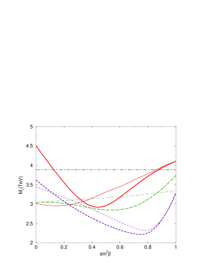
Our numerical results are summarized in Figs. 1 and 2, which correspond to the cases considered in Eqs. (5.3) and (5.7) respectively.

Figure 1: Lower bounds on $M_{c}$ corresponding to the case $\varepsilon^{H_{1}}=\varepsilon^{H_{2}}=1$ and $\varepsilon^{\ell_{L}}=\varepsilon^{u_{R}}=\varepsilon^{d_{R}}=1$ (solid line), $\varepsilon^{q_{L}}=\varepsilon^{e_{R}}=1$ (long-dashed), $\varepsilon^{u_{R}}=\varepsilon^{d_{R}}=\varepsilon^{e_{R}}=1$ (short-dashed) and $\varepsilon^{q_{L}}=\varepsilon^{\ell_{L}}=1$ (dash-dotted). Straight (non-straight) lines correspond to SM (MSSM) 5D extensions.

Figure 2: Lower bounds on $M_{c}$ corresponding to the case $\varepsilon^{H_{1}}=1,\ \varepsilon^{H_{2}}=0$, $\varepsilon^{q_{L}}=\varepsilon^{\ell_{L}}=\varepsilon^{u_{R}}=1$ (solid), $\varepsilon^{H_{1}}=1,\,\varepsilon^{H_{2}}=0,\,\varepsilon^{q_{L}}=\varepsilon^{u_{R}}=\varepsilon^{e_{R}}=1$ (short-dashed), $\varepsilon^{H_{1}}=0,\,\varepsilon^{H_{2}}=1,\,\varepsilon^{q_{L}}=\varepsilon^{\ell_{L}}=\varepsilon^{d_{R}}=\varepsilon^{e_{R}}=1$ (long-dashed) and $\varepsilon^{H_{1}}=\varepsilon^{H_{2}}=0,\,\varepsilon^{q_{L}}=\varepsilon^{\ell_{L}}=\varepsilon^{u_{R}}=\varepsilon^{d_{R}}=\varepsilon^{e_{R}}=1$ (dash-dotted). Thin (thick) lines correspond to SM (MSSM) 5D extensions.

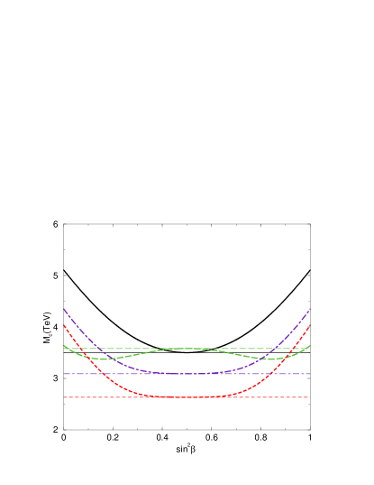
We could also relax the condition (5.2) and consider more general cases. They generically lead to bounds on $M_{c}$ of order a few TeV, as those in Figs. 1 and 2. However, some special cases can be constructed à la carte where the fit to the electroweak observables is particularly better than in the SM. To this end we can realize that the SM prediction for all observables in Table 1 lies close enough to the corresponding experimental value, except for the case of $Q_{W}$(Cs) whose SM prediction falls more than 2$\sigma$ away from the experimental result. Then new physics with $\delta\,Q_{W}>0$, and not touching significantly the rest of observables, is required. A quick glance at Eqs. (3.6), (4.4), (4.7) and (4.10) shows that this is indeed the case when $e_{R}$ and $d_{R}$ are on the brane, $\varepsilon^{e_{R}}=\varepsilon^{d_{R}}=1$, while all other fields, $H_{1,2}$, $u_{R}$, $q_{L}$ and $\ell_{L}$ live in the 5D bulk. In this case all observables in Table 1 are unmodified, except $Q_{W}$, which experiences a positive shift,

$$\delta\,Q_{W}=\frac{1}{12}\,(Z+2\,N)\,s^{2}_{\theta}\ X\,.$$ (5.8)

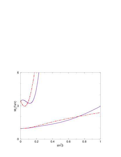
Now the fit to the observables of Table 1 has, with respect to the SM fit, $\Delta\chi^{2}\simeq-5.3$ and $\chi^{2}_{min}$ corresponds, using Eq. (5.8), to $M_{c}=1.30$ TeV, while the 95% c.l. upper and lower bounds are $0.95$ TeV $\leq M_{c}\leq 3.44$ TeV. Actually a model with these qualitative features is not unique. Even if one of the Higgs fields, e.g. $H_{2}$, lives in the bulk the contribution to $\delta\,Q_{W}$ can be positive and provide low values of the 95% c.l. lower (and even upper) bound. These cases are exemplified in Fig. 3, where the bounds are shown for the case in which only the fields $H_{2}$, $e_{R}$ and $d_{R}$ live on the boundary while the rest of the fields live in the bulk.

Figure 3: Lower (and upper) 95% c.l. bounds on $M_{c}$, as functions of $s^{2}_{\beta}$, for the case $\varepsilon^{H_{2}}=\varepsilon^{e_{R}}=\varepsilon^{d_{R}}=1$, and $\varepsilon^{H_{1}}=\varepsilon^{u_{R}}=\varepsilon^{\ell_{L}}=\varepsilon^{q_{L}}=0$. Solid (dash-dotted) lines correspond to the MSSM (SM) case.

6 Flavor and CP-violating physics

Up to now we have considered universality of KK interactions with respect to the different families of SM fermions. In this section we will consider the case where the different families of quarks and leptons are localized in different points of the extra dimension. This possibility has been motivated in order to explain the difference of masses of the families [16]. Also certain models from branes seem to lead to two families living in the bulk and one living on the boundary [17]. In all these situations one has flavor-violating interactions and therefore stronger bounds on $M_{c}$ coming from the experimental constraints on flavor and CP-violating physics. It is easy to understand how these flavor-violating interactions arise. The coupling of the gauge KK-excitations to the SM fermions is proportional to $\varepsilon^{\psi_{i}}\cos(nx_{5}/R)$, where $\varepsilon^{\psi_{i}}=1\ (0)$ for localized (not localized) fermions. Therefore if fermions live at different points of the extra dimension (or they have different $\varepsilon^{\psi_{i}}$), they will couple differently to the KK excitations, leading to flavor-violating couplings.

Let us consider in detail the case for the first two families. In the interaction basis, the flavor-violating couplings are given by (we only consider the KK excitations of the gluons $G^{A\,(n)}_{\mu}$ since they should provide the strongest constraint):

$$-{\cal L} = (\bar{d}_{R}\ \bar{s}_{R})V^{d\,\dagger}_{R}\left(\begin{array}[]{cc}m_{d}&0\\ 0&m_{s}\end{array}\right)V^{d}_{L}\left(\begin{array}[]{c}d_{L}\\ s_{L}\end{array}\right)+\frac{g}{\sqrt{2}}W_{\mu}(\bar{u}_{L}\ \bar{c}_{L})\gamma^{\mu}\left(\begin{array}[]{c}d_{L}\\ s_{L}\end{array}\right)$$ (6.7)

$$+ \sum_{n=1}^{\infty}\Bigg{[}\sqrt{2}g_{s}G^{A\,(n)}_{\mu}(\bar{d}_{L}\ \bar{s}_{L})\gamma^{\mu}T^{A}\left(\begin{array}[]{cc}c_{1}^{(n)}&0\\ 0&c_{2}^{(n)}\end{array}\right)\left(\begin{array}[]{c}d_{L}\\ s_{L}\end{array}\right)+(L\rightarrow R)\Bigg{]}$$ (6.12)

$$+ (d,s\leftrightarrow u,c)\,,$$ (6.13)

where $V^{d}_{L,R}$ are generic unitary matrices, and we have defined $c_{1,2}^{(n)}\equiv\varepsilon^{\psi_{1,2}}\cos\left(nx^{(1,2)}_{5}/R\right)$ where $x^{(1,2)}_{5}$ is the position, along the fifth dimension, of the left-handed quarks of the first and second family respectively. Going to the mass-eigenstate basis, we have

$$-{\cal L} = (\bar{d}_{R}\ \bar{s}_{R})\left(\begin{array}[]{cc}m_{d}&0\\ 0&m_{s}\end{array}\right)\left(\begin{array}[]{c}d_{L}\\ s_{L}\end{array}\right)+\frac{g}{\sqrt{2}}W_{\mu}(\bar{u}_{L}\ \bar{c}_{L})\gamma^{\mu}V^{u}_{L}V^{d\,\dagger}_{L}\left(\begin{array}[]{c}d_{L}\\ s_{L}\end{array}\right)$$ (6.20)

$$+ \sum_{n=1}^{\infty}\Bigg{[}\sqrt{2}g_{s}G^{A\,(n)}_{\mu}(\bar{d}_{L}\ \bar{s}_{L})\gamma^{\mu}T^{A}V^{d}_{L}\left(\begin{array}[]{cc}c_{1}^{(n)}&0\\ 0&c_{2}^{(n)}\end{array}\right)V_{L}^{d\,\dagger}\left(\begin{array}[]{c}d_{L}\\ s_{L}\end{array}\right)+(L\rightarrow R)\Bigg{]}$$ (6.25)

$$+ (d,s\leftrightarrow u,c)\,,$$ (6.26)

showing two sources of flavor violation, one from the CKM matrix $V^{u}_{L}V^{d\,\dagger}_{L}$ and another (if $c_{1}^{(n)}\not=c_{2}^{(n)}$) from

$$U^{d}_{L}\equiv V^{d}_{L}\left(\begin{array}[]{cc}c_{1}^{(n)}&0\\ 0&c_{2}^{(n)}\end{array}\right)V_{L}^{d\,\dagger}\,,$$ (6.27)

mediated by the KK gluons. Notice that for general $V^{u,d}_{L,R}$ the phases cannot be rotated away by field redefinitions and we can have CP violation with only two families.

The flavor-violating couplings of the KK gluons mediate flavor-changing neutral currents (FCNC) at tree level. For the down-type quarks the effective $\Delta S=2$ lagrangian mediated by the KK gluons is given by

$${\cal L}^{\Delta S=2}=\sum_{n=1}^{\infty}\frac{2g_{s}^{2}}{3n^{2}M^{2}_{c}}\left[U^{d}_{L\{12\}}\bar{d}_{L}\gamma^{\mu}s_{L}+(L\rightarrow R)+{\rm h.c.}\right]^{2}\,,$$ (6.28)

where by $U^{d}_{L\{ij\}}$ we denote the $\{ij\}$ element of the matrix $U^{d}_{L}$. From Eq. (6.27), we have using the unitarity of $V^{d}_{L}$

$$\sum_{n=1}^{\infty}\frac{U^{d\,2}_{L\{12\}}}{n^{2}}=\left(V^{d\,*}_{L\{21\}}V^{d\,}_{L\{11\}}\right)^{2}\sum_{n=1}^{\infty}\left(\frac{c_{1}^{(n)}-c_{2}^{(n)}}{n}\right)^{2}\,,$$ (6.29)

where the sum over the KK excitations is given by

$$\sum_{n=1}^{\infty}\left(\frac{c_{1}^{(n)}-c_{2}^{(n)}}{n}\right)^{2}=\left\{\begin{array}[]{ll}{\displaystyle\frac{\pi}{2\,R}\left|x^{(1)}_{5}-x^{(2)}_{5}\right|}&{\rm for}\ \varepsilon^{\psi_{1,2}}\not=0\\ &\\ {\displaystyle\frac{\pi^{2}}{24}+\frac{1}{2}\left(\frac{x^{(2)}_{5}}{R}-\frac{\pi}{2}\right)^{2}}&{\rm for}\ \varepsilon^{\psi_{1}}=0\,,\varepsilon^{\psi_{2}}\not=0\end{array}\right.\,.$$ (6.30)

Notice that the sum over $n$ in Eq. (6.30) is extended from $n=1$ to $n=\infty$, as was done in Eq. (2.3), although, properly speaking, it should have been extended up to $n\sim\Lambda\,R$, where $\Lambda$ is an effective ultraviolet cutoff related to the tension of the 4D brane. An equivalent way the cutoff appears is through the coupling of the $n$-KK to the brane fields, $g_{n}$, which can be computed and leads to an exponential drop-off as [1, 18]

$$g_{n}^{2}=g^{2}e^{-\frac{n^{2}}{\Lambda^{2}R^{2}}}\,.$$ (6.31)

The value of the cutoff $\Lambda$ has been studied in string theory, and in the effective theory of the brane world. It is found that $\Lambda=c\,\mu$, where $\mu$ is the tension of the brane and $c$ is a model-dependent coefficient [1, 18]. The sum in (2.3) and in (6.30) for $\varepsilon^{\psi_{1}}=0\,,\varepsilon^{\psi_{2}}\not=0$ is dominated by the contribution of the first $\sim$10 KK, and thus is not sensitive to the value of $\Lambda$. Equation (6.30) for $\varepsilon^{\psi_{1,2}}\not=0$ is also insensitive to the value of $\Lambda$, but only for large distances, $|x_{5}^{(1)}-x_{5}^{(2)}|\,\Lambda\gtrsim 1$. However, for small distances , $|x_{5}^{(1)}-x_{5}^{(2)}|\,\Lambda\lesssim 1$, and for values of the center-of-mass of the two branes $(x_{5}^{(1)}+x_{5}^{(2)})/2R=\mathcal{O}(1)$, the expression (6.30) should be replaced by

$$\sum_{n}\left(\frac{c_{1}^{(n)}-c_{2}^{(n)}}{n}\right)^{2}\simeq\frac{\Lambda}{2\,R}(x^{(1)}_{5}-x^{(2)}_{5})^{2}\ .$$ (6.32)

Armed with the lagrangian (6.28), we can calculate the contribution to $\Delta m_{K}$ and $\varepsilon_{K}$,

$$\Delta m_{K} = \frac{{\rm Re}\langle K|-{\cal L}^{\Delta S=2}|\bar{K}\rangle}{m_{K}}=3.5\times 10^{-15}\ {\rm GeV}\,,$$ (6.33)

$$\left|\varepsilon_{K}\right| = \frac{\left|{\rm Im}\langle K|-{\cal L}^{\Delta S=2}|\bar{K}\rangle\right|}{2\sqrt{2}m_{K}\Delta m_{K}}=2.3\times 10^{-3}\,.$$ (6.34)

Let us just consider the left-handed KK contribution to $\Delta m_{K}$ and $\varepsilon_{K}$. Requiring these to be smaller than the experimental value, we obtain respectively (using the vacuum-insertion approximation)

$$M_{c} \gtrsim 400\ {\rm TeV}\left(\frac{\sqrt{\sum_{n}{\rm Re}U^{d\,2}_{L\{12\}}/n^{2}}}{0.3}\right)\,,$$ (6.35)

$$M_{c} \gtrsim 5000\ {\rm TeV}\left(\frac{\sqrt{\sum_{n}{\rm Im}U^{d\,2}_{L\{12\}}/n^{2}}}{0.3}\right)\,,$$ (6.36)

where for the numerical bound we have assumed that the mixing angles $V^{d}_{L\{ij\}}$ are similar to those in the CKM matrix and that one family lives on the boundary ($c_{1}^{(n)}=1$) and the other in the bulk ($c_{2}^{(n)}=0$) so that Eq. (6.30) can be applied.

The constraints on $M_{c}$ for other scenarios can be easily read off from Eqs. (6.35) and (6.36). For example, let us consider the case in which the first and second families are localized at different points of the extra dimension. This could nicely explain the smallness of their masses, since mass terms can only arise from exponentially small overlaps of the wave functions of the fields [16]:

$$M_{d\ \{ij\}}\simeq e^{-\mu^{2}|\bar{x}^{(i)}_{5}-x^{(j)}_{5}|^{2}/2}\ v\,,$$ (6.37)

where $\bar{x}^{(i)}_{5}$ refers to the position in the extra dimension of the right-handed $i$ quark and $x^{(j)}_{5}$ to the position of the left-handed $j$ quark. Requiring that $M_{d\ \{22\}}=m_{s}$ and $M_{d\ \{21\}}=m_{s}s_{\theta_{C}}$ ($s_{\theta_{C}}\simeq 0.22$ is the Cabibbo angle), we have that the distance between the $s_{L}$ and $d_{L}$ is

$$|x^{(1)}_{5}-x^{(2)}_{5}|\simeq\frac{\sqrt{2}}{\mu}\left[\ln^{1/2}\left(\frac{v}{m_{s}s_{\theta_{C}}}\right)-\ln^{1/2}\left(\frac{v}{m_{s}}\right)\right]\simeq 0.4\mu^{-1}\,.$$ (6.38)

Using Eq. (6.32), we have from Eqs. (6.35) and (6.36) respectively the bounds

$$M_{c} \gtrsim 25\ {\rm TeV}\sqrt{10\Lambda/R\mu^{2}}\,,$$ (6.39)

$$M_{c} \gtrsim 300\ {\rm TeV}\sqrt{10\Lambda/R\mu^{2}}\,,$$ (6.40)

where we have normalized the bound to the case $\mu\sim\Lambda$ and $\Lambda R\sim 10$. These bounds are quite strong and disfavor this type of scenarios in models with TeV-string scale. On the same footing, we can also get constraints from the up-type quark sector. Since $(\Delta m_{D}/m_{D})_{exp}\simeq 10\,(\Delta m_{K}/m_{K})_{exp}$, we get a constraint that is a factor of $\sim 0.3$ weaker than that in Eq. (6.35).

The KK excitations of the gluon can also induce $\Delta S=1$ terms in the lagrangian that contribute to $\varepsilon^{\prime}_{K}/\varepsilon_{K}$. We find that the dominant contribution is given by

$$\left|\frac{\varepsilon^{\prime}_{K}}{\varepsilon_{K}}\right| \simeq \frac{\omega}{\sqrt{2}\left|\varepsilon_{K}\right|{\rm Re}A_{0}}\sum_{n}\frac{g^{2}_{s}}{n^{2}M^{2}_{c}}{\rm Im}\Bigg{\{}\frac{U^{d}_{L\,\{12\}}}{12}\Big{[}(U^{u}_{R\,\{11\}}+2U^{d}_{R\,\{11\}})\,\langle(\pi\pi)_{I=0}|Q_{6}|K\rangle$$ (6.41)

$$- \frac{2}{\omega}(U^{u}_{R\,\{11\}}-U^{d}_{R\,\{11\}})\,\langle(\pi\pi)_{I=2}|Q_{8}|K\rangle\Big{]}\Bigg{\}}\,,$$

where we follow the notation of Ref. [19]. Note that, since $\omega\simeq 1/22$, the second term of Eq. (6.41) gives the dominant contribution if there is isospin breaking in the right-handed sector (i.e. $U^{u}_{R}\not=U^{d}_{R}$). This is the case whenever the $u_{R}$ and the $d_{R}$ live in different points of the extra dimension. Considering this latter case, e.g. $U^{d}_{R\{11\}}\gg U^{u}_{R\{11\}}$, we obtain from Eq. (6.41) and $\left|\varepsilon^{\prime}_{K}/\varepsilon_{K}\right|_{exp}<2.5\times 10^{-3}$:

$$M_{c}\gtrsim 150\ {\rm TeV}\left(\frac{\sqrt{\sum_{n}{\rm Im}[U^{d}_{L\,\{12\}}U^{d}_{R\,\{11\}}]/n^{2}}}{0.6}\right)\,.$$ (6.42)

This bound is not competitive with that from $\varepsilon_{K}$ [Eq. (6.36)] if the mixing angles in $U^{d}_{L}$ are of order $s_{\theta_{C}}$. Nevertheless, since the bound from Eq. (6.42) scales as the square-root of the mixing angle, instead of linearly as that in Eq. (6.36), we have that for small mixings, i.e. Im$\{U^{d}_{L\,\{12\}}\}\lesssim 2\times 10^{-4}$, the bound (6.42) becomes the strongest one. In other words, sizeable contributions to both $\varepsilon^{\prime}_{K}/\varepsilon_{K}$ and $\varepsilon_{K}$ from KK gluons occurs for Im$\{U^{d}_{L\,\{12\}}\}\sim 2\times 10^{-4}$ and $M_{c}\sim 4$ TeV.

For models where only the third family lives in another point of the space ($c_{1}^{(n)}=c_{2}^{(n)}\not=c_{3}^{(n)}$), the above bounds also apply, with the only difference that now Eq. (6.29) must incorporate the third family. One obtains

$$\sum_{n=1}^{\infty}\frac{U^{d\,2}_{L\{12\}}}{n^{2}}=\left(V^{d\,*}_{L\{23\}}V^{d}_{L\{13\}}\right)^{2}\sum_{n=1}^{\infty}\left(\frac{c_{1}^{(n)}-c_{3}^{(n)}}{n}\right)^{2}\,.$$ (6.43)

For mixing angles similar to those in the CKM matrix (Im$\{V^{d}_{L\{23\}}V^{d}_{L\{13\}}\}\sim 2\times 10^{-4}$) we get from Eq. (6.42)

$$M_{c}\gtrsim 4\ {\rm TeV}\,.$$ (6.44)

It is interesting to remark that in this case the contribution to $\varepsilon_{K}$ and $\varepsilon^{\prime}_{K}/\varepsilon_{K}$ are both saturated for similar values of the compactification scale, $M_{c}\sim 4$ TeV. $B$ physics can also put constraints on $M_{c}$. From the experimental value of $\Delta m_{B}$, we obtain

$$M_{c}\gtrsim 2\ {\rm TeV}\left(\frac{\sqrt{\sum_{n}{\rm Re}\,U^{d\,2}_{L\{13\}}/n^{2}}}{0.005}\right)\,,$$ (6.45)

where again we have considered that the mixing angles between the first and third families are similar to those in the CKM matrix.

Let us finally consider the lepton sector. Bounds on family-violating couplings can be obtained, for example, from the experimental upper bound on BR$(\mu\rightarrow 3e)$. If the $\mu$ and $e$ live in different points, there will be a family transition $\mu-e$ mediated by the KK excitations of the $W_{3}$. We obtain

$${\rm BR}(\mu\rightarrow 3e)=\left|\sum_{n}\frac{\sqrt{2}m^{2}_{W}}{n^{2}M_{c}^{2}}U^{\ell}_{L\{21\}}U^{\ell}_{L\{11\}}\right|^{2}\,,$$ (6.46)

where now the mixing angles refer to the ones in the lepton sector. From BR$(\mu\rightarrow 3e)_{exp}<10^{-12}$ we obtain the bound

$$M_{c}\gtrsim 30\ {\rm TeV}\left(\frac{\sqrt{\sum_{n}|U^{\ell}_{L\{21\}}U^{\ell}_{L\{11\}}|/n^{2}}}{0.3}\right)\,,$$ (6.47)

where for the numerical estimate we assumed $c_{1}^{(n)}=1$ and $c_{2}^{(n)}=0$ and $|V^{\ell}_{L\{11\}}|\simeq 1$, $|V^{\ell}_{L\{21\}}|\sim\sqrt{m_{e}/m_{\mu}}\simeq 0.07$.

7 Conclusion

In this paper we have studied the implications of a TeV^-1 size dimension, where SM gauge-bosons propagate, on electroweak and flavor physics. This work generalizes those existing in the literature in two aspects:

• We have allowed for the possibility that the different fermions (as well as Higgs fields) live in the bulk of the extra dimension or are localized at different points of it, whereas previous analyses had only considered the case where all SM fermions are stuck at the boundary of the extra dimension.

• We have analyzed the extension of the SM to five dimensions and its minimal supersymmetric generalization. We have found interesting tree-level effects associated to the presence of supersymmetric partners. Previous analyses in the literature only considered the case of the 5D SM extensions.

Concerning the possibility of different locations for the different fermions, we have considered a wide variety of cases. Assuming universality in family space, we have seen that the lower bound on $M_{c}$ is very model-dependent, but it is generically around $2$–$5$ TeV. Nevertheless, we have found particular models where the correction to the weak charge $Q_{W}$ is positive, as required by the experimental data, whereas the other observables are unchanged. These cases provide a global fit to the electroweak observables better than that of the SM. The model with the best fit yields the 95% c.l. region: $0.95\,{\rm TeV}\lesssim\,M_{c}\lesssim 3.44\,{\rm TeV}$.

In the 5D supersymmetric case, we have found that one of the supersymmetric partners is a scalar SU(2)_L-triplet that acquires a VEV of $\mathcal{O}(RM_{Z})$ whenever a Higgs lives on the 4D boundary. This VEV modifies the SM relation between the $Z$ and $W$ masses and consequently the analysis of the global fit to the electroweak data. We find very different bounds on $M_{c}$ from the non-supersymmetric case.

Giving up lepton and quark universality and allowing the different families to be located at different points of the fifth dimension, we found that the KK excitations generate dangerous FCNC at the tree level. The effect on flavor observables such as $\Delta m_{K}$, $\varepsilon_{K}$ and $\varepsilon^{\prime}_{K}$, provides very stringent limits on $M_{c}$, as strong as $\sim 5000$ TeV. This seems to disfavor this type of scenarios in the context of TeV-strings.

We want to conclude by stressing some of the importance of the analysis carried out here. If indirect effects of an extra dimension (such as those considered here) put already strong bounds on $M_{c}$, it will make very unlikely the direct detection of the KK excitations of a SM field in future colliders [20, 9]. This would be the real test of an extra dimension. Combining the analysis here with that in Ref. [20, 9], one learns that only the LHC, that will probe KK excitations up to $6$–$7$ TeV, has a chance to discover an extra dimension. If the extra dimension treats families in a non-universal way, the bounds found here put the size of the extra dimension far from the experimental reach.

References

• [1] I. Antoniadis, Phys. Lett. B246 (1990) 377; I. Antoniadis, C. Muñoz and M. Quirós, Nucl. Phys. B397 (1993) 515; I. Antoniadis, K. Benakli and M. Quirós, Phys. Lett. B331 (1994) 313; I. Antoniadis and K. Benakli, Phys. Lett. B326 (1994) 69; K. Benakli, Phys. Lett. B386 (1996) 106; I. Antoniadis and M. Quirós, Phys. Lett. B392 (1997) 61; E. Cáceres, V.S. Kaplunovsky and I.M. Mandelberg, Nucl. Phys. B493 (1997) 73.
• [2] J.D. Lykken, Phys. Rev. D54 (1996) 3693.
• [3] N. Arkani-Hamed, S. Dimopoulos and G. Dvali, Phys. Lett. B429 (1998) 263; I. Antoniadis, N. Arkani-Hamed, S. Dimopoulos and G. Dvali, Phys. Lett. B436 (1998) 257.
• [4] I. Antoniadis and B. Pioline, hep-ph/9902055; K. Benakli and Y. Oz, hep-th/9910090.
• [5] S.C. Bennett and C.E. Wieman, Phys. Rev. Lett. 82 (1999) 2484.
• [6] R. Casalbuoni, S. De Curtis, D. Dominici and R. Gatto, Phys. Lett. B460 (1999) 135; J.L. Rosner, hep-ph/9907524; J. Erler and P. Langacker, hep-ph/9910315.
• [7] P. Nath and M. Yamaguchi, hep-ph/9902323.
• [8] M. Masip and A. Pomarol, Phys. Rev. D60 (1999) 096005.
• [9] T.G. Rizzo and J.D. Wells, hep-ph/9906234.
• [10] W.J. Marciano, Phys. Rev. D60 (1999) 093006; A. Strumia, hep-ph/9906266; R. Casalbuoni, S. De Curtis, D. Dominici and R. Gatto, hep-ph/9907355; C.D. Carone, hep-ph/9907362; F. Cornet, M. Relano and J. Rico, hep-ph/9908299.
• [11] A. Pomarol and M. Quirós, Phys. Lett. B438 (1998) 255; I. Antoniadis, S. Dimopoulos, A. Pomarol and M. Quirós, Nucl. Phys. B544 (1999) 503; A. Delgado, A. Pomarol and M. Quirós, Phys. Rev. D60 (1999) 095008.
• [12] E.A. Mirabelli and M. Peskin, Phys. Rev. D58 (1998) 065002.
• [13] C. Caso et al., Eur. Phys. J. C3 (1998) 1; J. Mnich, talk presented at EPS-HEP 99, Tampere (Finland), http://neutrino.pc.helsinki.fi/hep99/transparencies/Plenary/.
• [14] W.J. Marciano and A. Sirlin, Phys. Rev. D35 (1987) 1672.
• [15] G.J. Feldman and R.D. Cousins, Phys. Rev. D57 (1998) 3873.
• [16] N. Arkani-Hamed and M. Schmaltz, hep-ph/9903417.
• [17] G. Shiu and S.H. Tye, Phys. Rev. D58 (1999) 106007.
• [18] M. Bando, T. Kugo, T. Noguchi and K. Yoshioka, hep-ph/9906549; J. Hisano and N. Okada, hep-ph/9909555.
• [19] G. Buchalla, A.J. Buras and M.E. Lautenbacher, Rev. Mod. Phys. 68 (1996) 1125.
• [20] I. Antoniadis, K. Benakli and M. Quiros, hep-ph/9905311; P. Nath, Y. Yamada and M. Yamaguchi, hep-ph/9905415; T.G. Rizzo, hep-ph/9909232.