TUM-HEP-361/99
MPI-PhT/99-53
October 1999

Electroweak Penguin Contributions to
Non-Leptonic $\Delta F=1$ Decays at NNLO

Andrzej J. Buras¹, Paolo Gambino¹ and Ulrich A. Haisch^1,2

¹Technische Universität München,
Physik Dept., D-85748 Garching, Germany

²Max Planck Institut für Physik – Werner-Heisenberg-Institut,
Föhringer Ring 6, D-80805 Munich, Germany

Abstract

We calculate the ${\cal O}(\alpha_{s})$ corrections to the $Z^{0}$-penguin and electroweak box diagrams relevant for non-leptonic $\Delta F=1$ decays with $F=S,B$. This calculation provides the complete ${\cal O}(\alpha_{\scriptscriptstyle W}\alpha_{s})$ and ${\cal O}(\alpha_{\scriptscriptstyle W}\alpha_{s}\sin^{2}\theta_{\scriptscriptstyle W}m_{t}^{2})$ corrections ($\alpha_{\scriptscriptstyle W}=\alpha/\sin^{2}\theta_{\scriptscriptstyle W}$) to the Wilson coefficients of the electroweak penguin four quark operators relevant for non-leptonic K- and B-decays. We argue that this is the dominant part of the next-next-to-leading (NNLO) contributions to these coefficients. Our results allow to reduce considerably the uncertainty due to the definition of the top quark mass present in the existing NLO calculations of non-leptonic decays. The NNLO corrections to the coefficient of the color singlet $(V-A)\otimes(V-A)$ electroweak penguin operator $Q_{9}$ relevant for $B$-decays are generally moderate, amount to a few percent for the choice $m_{t}(\mu_{t}=m_{t})$ and depend only weakly on the renormalization scheme. Larger NNLO corrections with substantial scheme dependence are found for the coefficients of the remaining electroweak penguin operators $Q_{7}$, $Q_{8}$ and $Q_{10}$. In particular, the strong scheme dependence of the NNLO corrections to $C_{8}$ allows to reduce considerably the scheme dependence of $C_{8}\langle Q_{8}\rangle_{2}$ relevant for the ratio $\varepsilon^{\prime}/\varepsilon$.

1 Introduction

Electroweak penguin operators govern rare semi-leptonic decays such as $K\to\pi\nu\bar{\nu}$, $K_{L}\to\pi^{0}e^{+}e^{-}$, $B\to\pi\nu\bar{\nu}$ and $B_{s,d}\to\mu\bar{\mu}$ and contribute sometimes in an important manner to non-leptonic K- and B- decays. Among the latter one should mention the CP-violating ratio $\varepsilon^{\prime}/\varepsilon$ in $K_{L}\to\pi\pi$ decays and electroweak contributions to two-body decays like $B\to\pi K$, $B_{s}\to\pi^{0}\phi$ etc. [1].

The effective weak Hamiltonian for these decays has the following generic structure [2]

$${\cal H}_{eff}=\frac{G_{F}}{\sqrt{2}}\sum_{i}V^{i}_{\rm CKM}C_{i}(\mu)Q_{i}~{}.$$ (1.1)

Here $G_{F}$ is the Fermi constant and $Q_{i}$ are the relevant local operators which, in addition to electroweak penguin operators, include current-current operators, QCD-penguin operators and magnetic penguin operators. The Cabibbo-Kobayashi-Maskawa factors $V^{i}_{CKM}$ and the Wilson coefficients $C_{i}$ describe the strength with which a given operator enters the Hamiltonian. The decay amplitude for a decay of a meson M to a final state F is simply given by $\langle F|{\cal H}_{eff}|M\rangle$.

The renormalization scale ($\mu$) dependence of $\vec{C}^{T}(\mu)=(C_{1}(\mu),...)$ is governed by the renormalization group equation (RGE) whose solution is given by

$$\vec{C}(\mu)=\left[T_{g}\exp\int^{g_{s}(\mu)}_{g_{s}(\mu_{W})}dg_{s}^{\prime}{\hat{\gamma}^{T}(g_{s}^{\prime},\alpha)\over\beta(g_{s}^{\prime})}\right]\vec{C}(\mu_{W})\,,$$ (1.2)

where $T_{g}$ is the $g$-ordering operator, $\mu_{W}={\cal O}(M_{\scriptscriptstyle W})$ and $\mu$ is ${\cal O}(m_{\rm b})$ and ${\cal O}(1\mbox{ GeV})$ for B-decays and K-decays respectively. $\beta(g_{s})$ governs the evolution of the QCD coupling constant $g_{s}$ and $\hat{\gamma}$ is the anomalous dimension matrix which depends on the QED coupling constant $\alpha$ in addition to $\alpha_{s}=g_{s}^{2}/4\pi$. In what follows we will work to first order in $\alpha$.

Now, the initial conditions $\vec{C}(\mu_{W})$ are linear combinations of the so called Inami-Lim functions [3] such as $B_{0}(x_{t})$ with $x_{t}=m_{t}^{2}/M_{\scriptscriptstyle W}^{2}$ resulting from box diagrams, $C_{0}(x_{t})$ from $Z^{0}$-penguin diagrams, $D_{0}(x_{t})$ from the photon penguin diagrams, $E_{0}(x_{t})$ from the gluon penguin diagrams etc. The full list of functions including also those relevant for $\Delta S=2$, $\Delta B=2$ transitions and for radiative B- decays can be found in [4]. We will give explicit expressions for some of these functions below.

As shown in [5] any decay amplitude can then be written as a linear combination of the Inami-Lim functions to be denoted by $F^{(0)}_{r}(x_{t})$

$$A({\rm decay})=P_{0}({\rm decay})+\sum_{r}P_{r}({\rm decay})\,F^{(0)}_{r}(x_{t})\,,$$ (1.3)

where the sum runs over all functions contributing to a given decay and $P_{0}$ summarizes contributions from internal up and charm quarks. The process dependent coefficients $P_{r}$ include the effect of the renormalization group evolution from $\mu_{W}$ down to $\mu$ given in (1.2) as well the matrix elements of the operators $Q_{i}$. On the other hand the Inami-Lim functions $F^{(0)}_{r}(x_{t})$ are process independent. That is for instance the functions $B_{0}$ and $C_{0}$ enter both the semi-leptonic rare decays $K\to\pi\nu\bar{\nu}$ and $\varepsilon^{\prime}/\varepsilon$ which is related to non-leptonic decays $K_{L}\to\pi\pi$.

This Penguin-Box Expansion is very well suited for the study of the extensions of the Standard Model (SM) in which new particles are exchanged in the loops. We know already that these particles are relatively heavy and consequently they can be integrated out together with the weak bosons and the top quark. If there are no new local operators the mere change is to modify the functions $F^{(0)}_{r}(x_{t})$ which now acquire the dependence on the masses of new particles such as charged Higgs bosons and supersymmetric partners. The process dependent coefficients $P_{0}$ and $P_{r}$ remain unchanged unless new effective operators with different Dirac and color structures have to be introduced.

Now, the universal Inami-Lim functions $F^{(0)}_{r}(x_{t})$ result from one-loop box and penguin diagrams without QCD corrections and it is of interest to ask how these functions are modified when ${\cal O}(\alpha_{s})$ corrections to box and penguin diagrams are included.

The interest in answering this question is as follows:

• The estimate of the size of QCD corrections to the relevant decay branching ratios.

• The reduction of various unphysical scale dependences. In the case studied in this paper, this is in particular the dependence of QCD corrections on the scale $\mu_{t}$ at which the running top quark mass is defined. As some of the functions $F^{(0)}_{r}(x_{t})$ depend strongly on $m_{t}$, their $\mu_{t}$ dependence may result in the uncertainties as large as $\pm 15\%$ in the corresponding branching ratios. Only by calculating QCD corrections to box and penguin diagrams can this dependence be reduced.

• The universality of the top dependent functions can be violated by ${\cal O}(\alpha_{s})$ corrections. For instance in the case of semi-leptonic FCNC transitions there is no gluon exchange in a $Z^{0}$-penguin diagram parallel to the $Z^{0}$-propagator but such an exchange takes place in non-leptonic decays in which all external particles are quarks. The same applies to box diagrams contributing to $K\to\pi\nu\bar{\nu}$ and $\varepsilon^{\prime}/\varepsilon$ respectively. It is of interest then to find out whether the breakdown of the universality is substantial.

• Most importantly, however, the inclusion of ${\cal O}(\alpha_{s})$ corrections to penguin and box diagrams relevant for non-leptonic decays justifies the simultaneous inclusion of particular next-next-to-leading (NNLO) QCD corrections to the renormalization group transformation in (1.2). In the case of the electroweak penguin operator $Q_{8}$ (see (2.5)), relevant for $\varepsilon^{\prime}/\varepsilon$, this results in a welcome renormalization scheme dependence of $C_{8}(\mu)$ which in turn allows to reduce considerably the renormalization scheme dependence of $\varepsilon^{\prime}/\varepsilon$ present at NLO.

So far the following ${\cal O}(\alpha_{s})$ corrections to box and penguin diagrams have been calculated:

• ${\cal O}(\alpha_{s})$ corrections to $Z^{0}$-penguin function $C_{0}$ and to the box-diagram function $B_{0}$ in the case of rare semi-leptonic decays like $K\to\pi\nu\bar{\nu}$, $B\to\mu\bar{\mu}$ etc. [6, 7, 8]

• ${\cal O}(\alpha_{s})$ corrections to chromomagnetic and magnetic penguins relevant for radiative decays $B\to X_{s}\gamma$ and $B\to X_{s}l^{+}l^{-}$ [9, 10, 11, 12].

• ${\cal O}(\alpha_{s})$ corrections to the photon penguin function $D_{0}$ relevant for $B\to X_{s}l^{+}l^{-}$ and $K_{L}\to\pi^{0}l^{+}l^{-}$ [13].

• ${\cal O}(\alpha_{s}^{2})$ corrections to the matching conditions of all the operators $Q_{1-6}$, including the ${\cal O}(\alpha_{s})$ contributions to the gluon penguin function $E_{0}$ [13].

The purpose of the present paper is the calculation of ${\cal O}(\alpha_{s})$ corrections to $Z^{0}$-penguin and box-diagrams relevant for non-leptonic decays, such as two-body B-meson decays and $K_{L}\to\pi\pi~{}(\varepsilon^{\prime}/\varepsilon)$. This will allow to reduce the $\mu_{t}$-dependence in the NLO expressions present in the literature, to investigate the breakdown of the universality of the relevant Inami-Lim functions and to study the renormalization scheme dependence at the NNLO level.

As we will discuss explicitly in Section 3 the QCD corrections calculated here are a part of the complete next-next-to-leading (NNLO) corrections to non-leptonic decays in a renormalization group improved perturbation theory. In order to complete the NNLO calculations of the relevant Wilson coefficients one would have to calculate ${\cal O}(\alpha_{s}^{2})$ corrections to QCD penguin diagrams and in particular perform three-loop calculations ${\cal O}(\alpha_{s}^{3})$, ${\cal O}(\alpha\alpha_{s}^{2})$ of the anomalous dimensions of the full set of operators, which is a formidable task and clearly beyond the scope of our paper. However our calculation is sufficient to obtain the complete ${\cal O}(\alpha_{\scriptscriptstyle W}\alpha_{s})$ and the ${\cal O}(\alpha_{\scriptscriptstyle W}\alpha_{s}\sin^{2}\theta_{\scriptscriptstyle W}m_{t}^{2})$ corrections to the Wilson coefficients $C_{7-10}(\mu)$ of the electroweak penguin operators where $\alpha_{\scriptscriptstyle W}=\alpha/\sin^{2}\theta_{\scriptscriptstyle W}$. It is also sufficient to investigate the issue of the $\mu_{t}$-dependence of these coefficients and of its reduction through ${\cal O}(\alpha_{s})$ corrections calculated here. Finally it allows to analyze the breakdown of the universality in the Inami-Lim functions related to $Z^{0}$-penguin and box diagrams.

Our paper is organized as follows. In Section 2 we recall the known effective Hamiltonian for $\Delta S=1$ decays at the NLO level. We list the contributing operators and give the expressions for the Inami-Lim functions. In Section 3 we discuss our paper in the context of a complete NNLO calculation, we motivate our approximations and we outline the strategy. In Section 4 we elaborate on the renormalization scheme dependence. The calculation of the gluonic corrections to the $Z^{0}$ penguin diagrams and to the electroweak box diagrams is described in Sections  5 and 6, respectively. In Section 7 we collect the results in terms of ${\cal O}(\alpha_{\scriptscriptstyle W}\alpha_{s})$ contributions to the Wilson coefficients $C_{7-10}(M_{\scriptscriptstyle W})$ and discuss their numerical relevance at various scales, as well as the residual scale and scheme dependences. Finally, in Section 8 we summarize our paper and we briefly discuss the impact of our findings on the phenomenology of non-leptonic decays.

2 Notation and Conventions

In this section we establish our notation and recall some definitions that will be useful in the rest of the paper. We give explicit formulae for $\Delta S=1$ decays. It is straightforward to transform them to the $\Delta B=1$ case. The effective Hamiltonian for $\Delta S=1$ transitions can be written as [2]:

$${\cal H}_{\rm eff}(\Delta S=1)=-\frac{G_{\rm F}}{\sqrt{2}}\,V_{ts}^{*}V_{td}\,\sum_{i=1}^{10}C_{i}(\mu)\,Q_{i}(\mu),$$ (2.1)

where we have dropped the terms proportional to $V_{us}^{*}V_{ud}$ which are of no concern to us here. In [2] $C_{i}(\mu)\equiv y_{i}(\mu)$. The operators $Q_{i}$ are given explicitly as follows:

Current–Current :

$$Q_{1}=(\bar{s}_{\alpha}u_{\beta})_{V-A}\;(\bar{u}_{\beta}d_{\alpha})_{V-A}~{}~{}~{}~{}~{}~{}Q_{2}=(\bar{s}u)_{V-A}\;(\bar{u}d)_{V-A}$$ (2.2)

QCD–Penguins :

$$Q_{3}=(\bar{s}d)_{V-A}\sum_{q=u,d,s}(\bar{q}q)_{V-A}~{}~{}~{}~{}~{}~{}Q_{4}=(\bar{s}_{\alpha}d_{\beta})_{V-A}\sum_{q=u,d,s}(\bar{q}_{\beta}q_{\alpha})_{V-A}$$ (2.3)

$$Q_{5}=(\bar{s}d)_{V-A}\sum_{q=u,d,s}(\bar{q}q)_{V+A}~{}~{}~{}~{}~{}Q_{6}=(\bar{s}_{\alpha}d_{\beta})_{V-A}\sum_{q=u,d,s}(\bar{q}_{\beta}q_{\alpha})_{V+A}$$ (2.4)

Electroweak–Penguins :

$$Q_{7}={3\over 2}\;(\bar{s}d)_{V-A}\sum_{q=u,d,s}e_{q}\;(\bar{q}q)_{V+A}~{}~{}~{}~{}~{}Q_{8}={3\over 2}\;(\bar{s}_{\alpha}d_{\beta})_{V-A}\sum_{q=u,d,s}e_{q}(\bar{q}_{\beta}q_{\alpha})_{V+A}$$ (2.5)

$$Q_{9}={3\over 2}\;(\bar{s}d)_{V-A}\sum_{q=u,d,s}e_{q}(\bar{q}q)_{V-A}~{}~{}~{}~{}~{}Q_{10}={3\over 2}\;(\bar{s}_{\alpha}d_{\beta})_{V-A}\sum_{q=u,d,s}e_{q}\;(\bar{q}_{\beta}q_{\alpha})_{V-A}\,.$$ (2.6)

Here, $e_{q}$ denotes the electrical quark charges reflecting the electroweak origin of $Q_{7},\ldots,Q_{10}$. The initial conditions for the Wilson coefficients $C_{i}$ at $\mu=M_{\scriptscriptstyle W}$ obtained from the one-loop matching of the full to the effective theory are given in the NDR renormalization scheme as follows [14]:

$$C_{1}(M_{\scriptscriptstyle W}) = \frac{11}{2}\;\frac{\alpha_{s}(M_{\scriptscriptstyle W})}{4\pi}\,,$$ (2.7)

$$C_{2}(M_{\scriptscriptstyle W}) = 1-\frac{11}{6}\;\frac{\alpha_{s}(M_{\scriptscriptstyle W})}{4\pi}-\frac{35}{18}\;\frac{\alpha}{4\pi}\,,$$ (2.8)

$$C_{3}(M_{\scriptscriptstyle W}) = -\frac{\alpha_{s}(M_{\scriptscriptstyle W})}{24\pi}\widetilde{E}_{0}(x_{t})+\frac{\alpha_{\scriptscriptstyle W}}{6\pi}\left[2B_{0}(x_{t})+C_{0}(x_{t})\right]\,,$$ (2.9)

$$C_{4}(M_{\scriptscriptstyle W}) = \frac{\alpha_{s}(M_{\scriptscriptstyle W})}{8\pi}\widetilde{E}_{0}(x_{t})\,,$$ (2.10)

$$C_{5}(M_{\scriptscriptstyle W}) = -\frac{\alpha_{s}(M_{\scriptscriptstyle W})}{24\pi}\widetilde{E}_{0}(x_{t})\,,$$ (2.11)

$$C_{6}(M_{\scriptscriptstyle W}) = \frac{\alpha_{s}(M_{\scriptscriptstyle W})}{8\pi}\widetilde{E}_{0}(x_{t})\,,$$ (2.12)

$$C_{7}(M_{\scriptscriptstyle W}) = \frac{\alpha_{\scriptscriptstyle W}}{6\pi}\sin^{2}\theta_{\scriptscriptstyle W}\left[4C_{0}(x_{t})+\widetilde{D}_{0}(x_{t})\right]\,,$$ (2.13)

$$C_{8}(M_{\scriptscriptstyle W}) = 0\,,$$ (2.14)

$$C_{9}(M_{\scriptscriptstyle W}) = \frac{\alpha_{\scriptscriptstyle W}}{6\pi}\left[\sin^{2}\theta_{\scriptscriptstyle W}(4C_{0}(x_{t})+\widetilde{D}_{0}(x_{t}))+10B_{0}(x_{t})-4C_{0}(x_{t})\right]\,,$$ (2.15)

$$C_{10}(M_{\scriptscriptstyle W}) = 0\,,$$ (2.16)

where we have introduced $\alpha_{\scriptscriptstyle W}=g^{2}/4\pi=\alpha/\sin^{2}\theta_{\scriptscriptstyle W}$. $g$ is the weak coupling of $SU(2)_{L}$. We recall that

$$B_{0}(x_{t}) = \frac{1}{4}\left[\frac{x_{t}}{1-x_{t}}+\frac{x_{t}\ln x_{t}}{(x_{t}-1)^{2}}\right]\,,$$ (2.17)

$$C_{0}(x_{t}) = \frac{x_{t}}{8}\left[\frac{x_{t}-6}{x_{t}-1}+\frac{3x_{t}+2}{(x_{t}-1)^{2}}\ln x_{t}\right]\,,$$ (2.18)

$$D_{0}(x_{t}) = -\frac{4}{9}\ln x_{t}+\frac{-19x_{t}^{3}+25x_{t}^{2}}{36(x_{t}-1)^{3}}+\frac{x_{t}^{2}(5x_{t}^{2}-2x_{t}-6)}{18(x_{t}-1)^{4}}\ln x_{t}\,,$$ (2.19)

$$E_{0}(x_{t}) = -\frac{2}{3}\ln x_{t}+\frac{x_{t}(18-11x_{t}-x_{t}^{2})}{12(1-x_{t})^{3}}+\frac{x_{t}^{2}(15-16x_{t}+4x_{t}^{2})}{6(1-x_{t})^{4}}\,,$$ (2.20)

$$\widetilde{D}_{0}(x_{t}) = D_{0}(x_{t})-\frac{4}{9}\,,\ \ \ \ \ \ \ \ \ \widetilde{E}_{0}(x_{t})=E_{0}(x_{t})-\frac{2}{3}\,.$$ (2.21)

$B_{0}(x_{t})$ results from the evaluation of the box diagrams, $C_{0}(x_{t})$ from the $Z^{0}$-penguin, $D_{0}(x_{t})$ from the photon penguin diagrams and $E_{0}(x_{t})$ from QCD penguin diagrams. The constants $-4/9$ and $-2/3$ in (2.21) are characteristic for the NDR scheme. They are absent in the HV scheme. For $\mu\not=M_{\scriptscriptstyle W}$ non-vanishing $C_{8}$ and $C_{10}$ are generated through QCD effects. The formulae (2.7)-(2.16) apply also to the $\Delta B=1$ case with the appropriate change of fields in $Q_{i}$.

Let us next recall that in the leading order (LO) of the renormalization group improved perturbation theory in which $(\alpha_{s}t)^{n}$ and $\alpha t(\alpha_{s}t)^{n}$ terms with $t=\ln\,(M_{\scriptscriptstyle W}^{2}/\mu^{2})$ are summed only $C_{2}(M_{\scriptscriptstyle W})=1$ is different from zero. In particular $C_{7-10}(M_{\scriptscriptstyle W})=0$. The initial conditions given in (2.7)-(2.16) are appropriate to next-to-leading order (NLO) in which $\alpha_{s}(\alpha_{s}t)^{n}$ and $\alpha(\alpha_{s}t)^{n}$ terms are summed. In the next-next-to-leading order (NNLO) in which $\alpha_{s}^{2}(\alpha_{s}t)^{n}$ and $\alpha\alpha_{s}(\alpha_{s}t)^{n}$ are summed, ${\cal O}(\alpha_{s}^{2})$ terms in the initial conditions of $C_{1-6}(M_{\scriptscriptstyle W})$ and ${\cal O}(\alpha\alpha_{s})$ terms for all $C_{i}(M_{\scriptscriptstyle W})$ have to be included. In the present paper we will calculate the dominant ${\cal O}(\alpha\alpha_{s})$ corrections to the coefficients $C_{7-10}(M_{\scriptscriptstyle W})$ of the electroweak penguin operators. As we will discuss below this will be sufficient to sum the dominant contribution of the $\alpha\alpha_{s}(\alpha_{s}t)^{n}$ logarithms.

Finally we should stress that among ${\cal O}(\alpha\alpha_{s})$ terms we distinguish between ${\cal O}(\alpha_{\scriptscriptstyle W}\alpha_{s})$ and ${\cal O}(\alpha_{\scriptscriptstyle W}\alpha_{s}\sin^{2}\theta_{\scriptscriptstyle W})$ terms for reasons to be explained in detail below.

3 General Structure at NNLO and Strategy

Our aim is to compute the ${\cal O}(\alpha_{s})$ corrections to the $Z^{0}$-penguin diagrams and electroweak box diagrams relevant for non-leptonic $\Delta F=1$ decays. This calculation constitutes only a part of the complete computation of the Wilson coefficients $C_{i}(\mu)$ (i=1,…10) at NNLO in the renormalization group improved perturbation theory. On the other hand, as we will now demonstrate, our results combined with the known ${\cal O}(\alpha_{s})$ and ${\cal O}(\alpha_{s}^{2})$ anomalous dimensions of $Q_{i}$ provide the complete ${\cal O}(\alpha_{\scriptscriptstyle W}\alpha_{s})$ corrections to the Wilson coefficients $C_{7-10}(\mu)$ of the electroweak penguin operators not suppressed by $\sin^{2}\theta_{\scriptscriptstyle W}$ and the ${\cal O}(\alpha_{\scriptscriptstyle W}\alpha_{s}\sin^{2}\theta_{\scriptscriptstyle W})$ corrections quadratic in $m_{t}$ to these coefficients. These corrections turn out to be by far the dominant contributions to $C_{7-10}(\mu)$ at the NNLO level.

In order to prove these statements it is instructive to describe the computation of the Wilson coefficients $C_{i}(\mu)$ including LO, NLO and NNLO corrections. Generalizing the standard procedure at NLO [14, 4] to include NNLO corrections we proceed as follows.

Step 1: An amplitude for a properly chosen non-leptonic quark decay is calculated perturbatively in the full theory including all sorts of diagrams such as QCD penguin diagrams, electroweak penguin diagrams, box diagrams, W-boson exchanges and QCD corrections to all these diagrams. The result including LO, NLO and NNLO correction is given schematically as follows:

$$A_{full} \!\!=\!\! \langle\vec{Q}^{(0)}\rangle^{T}\left[\vec{A}^{(0)}+\frac{\alpha_{s}(M_{\scriptscriptstyle W})}{4\pi}\vec{A}_{s}^{(1)}+\left(\frac{\alpha_{s}(M_{\scriptscriptstyle W})}{4\pi}\right)^{2}\vec{A}_{s}^{(2)}+\frac{\alpha}{4\pi}\vec{A}_{e}^{(1)}+\frac{\alpha}{4\pi}\frac{\alpha_{s}(M_{\scriptscriptstyle W})}{4\pi}\vec{A}_{es}^{(2)}\right]$$ (3.1)

$$\!\!\equiv\!\! \langle\vec{Q}(M_{\scriptscriptstyle W})\rangle^{T}\vec{C}(M_{\scriptscriptstyle W})\,,$$

where $\langle\vec{Q}^{0}\rangle$ is a ten dimensional column vector built out of tree level matrix elements of the operators $Q_{i}$. The superscripts (0), (1) and (2) denote LO, NLO and NNLO contributions, respectively. The ${\cal O}(\alpha\alpha_{s})$ corrections include ${\cal O}(\alpha_{\scriptscriptstyle W}\alpha_{s})$, ${\cal O}(\alpha_{\scriptscriptstyle W}\alpha_{s}\sin^{2}\theta_{\scriptscriptstyle W})$ and ${\cal O}(\alpha_{\scriptscriptstyle W}\alpha_{s}\sin^{4}\theta_{\scriptscriptstyle W})$ terms.

Step 2: In order to extract the coefficients $\vec{C}(M_{\scriptscriptstyle W})$ from (3.1) one has to calculate the matrix elements of $Q_{i}$ between the same external quark states as in Step 1. This involves generally the computation of the operator insertions into the current-current, gluon penguin and photon penguin diagrams of the effective theory (W, top and $Z^{0}$ have been integrated out) together with QCD and QED corrections to these insertions. Including LO, NLO and NNLO corrections one finds

$$\langle\vec{Q}(M_{\scriptscriptstyle W})\rangle \!\!=\!\! \left[\hat{1}+\frac{\alpha_{s}(M_{\scriptscriptstyle W})}{4\pi}\hat{r}_{s}^{(1)}+\left(\frac{\alpha_{s}(M_{\scriptscriptstyle W})}{4\pi}\right)^{2}\hat{r}_{s}^{(2)}+\frac{\alpha}{4\pi}\hat{r}_{e}^{(1)}+\frac{\alpha}{4\pi}\frac{\alpha_{s}(M_{\scriptscriptstyle W})}{4\pi}\hat{r}_{es}^{(2)}\right]\langle\vec{Q}^{(0)}\rangle$$

with $\hat{r}_{i}$ being $10\times 10$ matrices. As $W$ and $Z^{0}$ have been integrated out only ${\cal O}(\alpha_{\scriptscriptstyle W}\alpha_{s}\sin^{2}\theta_{\scriptscriptstyle W})$ terms are present in ${\cal O}(\alpha\alpha_{s})$ corrections.

Step 3: From (3.1) and (3) we extract

$$\vec{C}(M_{\scriptscriptstyle W}) = \vec{C}^{(0)}+\frac{\alpha_{s}(M_{\scriptscriptstyle W})}{4\pi}\vec{C}_{s}^{(1)}+\left(\frac{\alpha_{s}(M_{\scriptscriptstyle W})}{4\pi}\right)^{2}\vec{C}_{s}^{(2)}+\frac{\alpha}{4\pi}\vec{C}_{e}^{(1)}+\frac{\alpha}{4\pi}\frac{\alpha_{s}(M_{\scriptscriptstyle W})}{4\pi}\vec{C}_{es}^{(2)}\,,\hskip 21.33955pt$$ (3.3)

where

$$\vec{C}^{(0)} = \vec{A}^{(0)}\hskip 5.69054pt=\hskip 5.69054pt(0,1,0,\ldots,0)^{T}\,,$$ (3.4)

$$\vec{C}_{s}^{(1)} = \vec{A}_{s}^{(1)}-\hat{r}_{s}^{(1)^{T}}\vec{C}^{(0)}\,,$$ (3.5)

$$\vec{C}_{e}^{(1)} = \vec{A}_{e}^{(1)}-\hat{r}_{e}^{(1)^{T}}\vec{C}^{(0)}\,,$$ (3.6)

$$\vec{C}_{s}^{(2)} = \vec{A}_{s}^{(2)}-\hat{r}_{s}^{(2)^{T}}\vec{C}^{(0)}-\hat{r}_{s}^{(1)^{T}}\vec{C}_{s}^{(1)}\,,$$ (3.7)

$$\vec{C}_{es}^{(2)} = \vec{A}_{es}^{(2)}-\hat{r}_{s}^{(1)^{T}}\vec{C}_{e}^{(1)}-\hat{r}_{es}^{(2)^{T}}\vec{C}^{(0)}-\hat{r}_{e}^{(1)^{T}}\vec{C}_{s}^{(1)}\,.$$ (3.8)

The electroweak penguin components of $\vec{C}_{e}^{(1)}$ and the components of $\vec{C}_{s}^{(1)}$ which contribute to the coefficients of the operators $Q_{1-6}$ are given explicitly in (2.7)-(2.16). $\vec{C}_{s}^{(2)}$ has been calculated in [13], but it contributes only to ${\cal O}(\alpha_{s}^{2})$ corrections to the coefficients of $Q_{1-6}$.

Among the four terms contributing to $\vec{C}_{es}^{(2)}$ only $\vec{A}_{es}^{(2)}$ and $\hat{r}_{s}^{(1)^{T}}\vec{C}_{e}^{(1)}$ are of interest to us as these are the only ones contributing to ${\cal O}(\alpha_{\scriptscriptstyle W}\alpha_{s})$ corrections and to ${\cal O}(\alpha_{\scriptscriptstyle W}\alpha_{s}\sin^{2}\theta_{\scriptscriptstyle W})$ corrections quadratic in $m_{t}$ which we aim to calculate. The third and fourth term in (3.8) contribute only to ${\cal O}(\alpha_{\scriptscriptstyle W}\alpha_{s}\sin^{2}\theta_{\scriptscriptstyle W})$ corrections. The third term is $m_{t}$-independent and unknown. The last term can be extracted from the known one-loop results but it has no dependence quadratic in $m_{t}$ and will not be included here.

The main purpose of this paper is then the two-loop calculation of $Z^{0}$-penguin and box diagrams giving $\vec{A}_{es}^{(2)}$. The contribution from the effective theory $\hat{r}_{s}^{(1)^{T}}\vec{C}_{e}^{(1)}$ can be extracted from the known one-loop results. In the case of the Wilson coefficients of electroweak penguin operators a simplification occurs as only the operator insertions in current-current topologies in $\hat{r}_{s}^{(1)^{T}}$ contribute. Were we interested also in the coefficients of the QCD-penguin operators, also the insertions into QCD-penguin and QED-penguin topologies would have to be retained.

Step 4: We use next the renormalization group transformation to find

$$\vec{C}(\mu)=\hat{U}(\mu,M_{\scriptscriptstyle W},\alpha)\vec{C}(M_{\scriptscriptstyle W})\,,$$ (3.9)

where

$$\hat{U}(\mu,M_{\scriptscriptstyle W},\alpha)=\hat{U}(\mu,M_{\scriptscriptstyle W})+\frac{\alpha}{4\pi}\left[\hat{R}^{(0)}(\mu,M_{\scriptscriptstyle W})+\hat{R}^{(1)}(\mu,M_{\scriptscriptstyle W})+\hat{R}^{(2)}(\mu,M_{\scriptscriptstyle W})\right]$$ (3.10)

with the pure QCD evolution given by

$$\hat{U}(\mu,M_{\scriptscriptstyle W})=\hat{U}^{(0)}(\mu,M_{\scriptscriptstyle W})+\hat{U}^{(1)}(\mu,M_{\scriptscriptstyle W})+\hat{U}^{(2)}(\mu,M_{\scriptscriptstyle W}).$$ (3.11)

The matrices $\hat{U}^{(i)}$ and $\hat{R}^{(i)}$ are functions of the anomalous dimension matrices of the operators in question and of the QCD beta function. Explicit expressions for $\hat{U}^{(0)}$, $\hat{U}^{(1)}$, $\hat{R}^{(0)}$ and $\hat{R}^{(1)}$ can be extracted from [14, 15]. $\hat{R}^{(2)}$ and $\hat{U}^{(2)}$ are not known as they require the evaluation of the three-loop anomalous dimension matrices ${\cal O}(\alpha\alpha_{s}^{2})$ and ${\cal O}(\alpha_{s}^{3})$, respectively. From the point of view of the expansion in $\alpha_{s}$ in the renormalization group improved perturbation theory, $\hat{U}^{(0)}$, $\hat{U}^{(1)}$ and $\hat{U}^{(2)}$ are ${\cal O}(1)$, ${\cal O}(\alpha_{s})$ and ${\cal O}(\alpha_{s}^{2})$, respectively. $\hat{R}^{(0)}$, $\hat{R}^{(1)}$ and $\hat{R}^{(2)}$ are ${\cal O}(1/\alpha_{s})$, ${\cal O}(1)$ and ${\cal O}(\alpha_{s})$, respectively.

Inserting (3.10) and (3.3) into (3.9) and expanding in $\alpha_{s}$ we find

$$\vec{C}(\mu)=\vec{C}_{s}(\mu)+\frac{\alpha}{4\pi}\left[\vec{C}_{I}(\mu)+\vec{C}_{II}(\mu)\right]~{}.$$ (3.12)

$\vec{C}_{s}(\mu)$ results from ${\cal O}(1)$, ${\cal O}(\alpha_{s})$ and ${\cal O}(\alpha_{s}^{2})$ terms in $\vec{C}(M_{\scriptscriptstyle W})$ and the QCD evolution $\hat{U}(\mu,M_{\scriptscriptstyle W})$. $\vec{C}_{I}(\mu)$ results from terms ${\cal O}(\alpha)$ and ${\cal O}(\alpha\alpha_{s})$ in $\vec{C}(M_{\scriptscriptstyle W})$ and $\hat{U}(\mu,M_{\scriptscriptstyle W})$. Finally $\vec{C}_{II}(\mu)$ is found by taking the contributions ${\cal O}(1)$, ${\cal O}(\alpha_{s})$ and ${\cal O}(\alpha_{s}^{2})$ in $\vec{C}(M_{\scriptscriptstyle W})$ and performing renormalization group transformation using $\hat{R}^{(i)}$. Explicitly we have:

$$\vec{C}_{s}(\mu) = \hat{U}^{(0)}(\mu,M_{\scriptscriptstyle W})\left[\vec{C}^{(0)}+\frac{\alpha_{s}(M_{\scriptscriptstyle W})}{4\pi}\vec{C}_{s}^{(1)}+\left(\frac{\alpha_{s}(M_{\scriptscriptstyle W})}{4\pi}\right)^{2}\vec{C}_{s}^{(2)}\right]$$ (3.13)

$$+ \hat{U}^{(1)}(\mu,M_{\scriptscriptstyle W})\left[\vec{C}^{(0)}+\frac{\alpha_{s}(M_{\scriptscriptstyle W})}{4\pi}\vec{C}_{s}^{(1)}\right]+\hat{U}^{(2)}(\mu,M_{\scriptscriptstyle W})\vec{C}^{(0)}\,,$$

$$\vec{C}_{I}(\mu)=\hat{U}^{(0)}(\mu,M_{\scriptscriptstyle W})\left[\vec{C}_{e}^{(1)}+\frac{\alpha_{s}(M_{\scriptscriptstyle W})}{4\pi}\vec{C}_{es}^{(2)}\right]+\hat{U}^{(1)}(\mu,M_{\scriptscriptstyle W})\vec{C}_{e}^{(1)}\,,$$ (3.14)

$$\vec{C}_{II}(\mu) = \hat{R}^{(0)}(\mu,M_{\scriptscriptstyle W})\left[\vec{C}^{(0)}+\frac{\alpha_{s}(M_{\scriptscriptstyle W})}{4\pi}\vec{C}_{s}^{(1)}+\left(\frac{\alpha_{s}(M_{\scriptscriptstyle W})}{4\pi}\right)^{2}\vec{C}_{s}^{(2)}\right]$$ (3.15)

$$+ \hat{R}^{(1)}(\mu,M_{\scriptscriptstyle W})\left[\vec{C}^{(0)}+\frac{\alpha_{s}(M_{\scriptscriptstyle W})}{4\pi}\vec{C}_{s}^{(1)}\right]+\hat{R}^{(2)}(\mu,M_{\scriptscriptstyle W})\vec{C}^{(0)}\,.$$

Let us now identify the ${\cal O}(\alpha_{\scriptscriptstyle W}\alpha_{s})$ contributions to electroweak penguin coefficients, calculated in subsequent sections, in this full NNLO result. They are fully contained in the last two terms in $\vec{C}_{I}(\mu)$. These two terms can be schematically decomposed as follows:

$$F_{1}(x_{t},\alpha_{s})+F_{2}(x_{t},\alpha_{s})\,\sin^{2}\theta_{\scriptscriptstyle W}\,.$$ (3.16)

The ${\cal O}(\alpha_{\scriptscriptstyle W}\alpha_{s})$ corrections are represented by the first term and our calculation provides the complete result for $F_{1}(x_{t},\alpha_{s})$. On the other hand, our calculation gives only a partial result for $F_{2}(x_{t},\alpha_{s})$ which is ${\cal O}(\alpha_{\scriptscriptstyle W}\alpha_{s}\sin^{2}\theta_{\scriptscriptstyle W})$. The contributions from gluon corrections to photon penguin diagrams and ${\cal O}(\alpha)$ corrections to QCD penguin diagrams which both contribute to $F_{2}(x_{t},\alpha_{s})$ are still missing in the case of non-leptonic decays. Similarly, some ${\cal O}(\alpha_{\scriptscriptstyle W}\alpha_{s}\sin^{2}\theta_{\scriptscriptstyle W})$ corrections contributing to the Wilson coefficient functions through $\vec{C}_{II}(\mu)$ are not known. Yet, as we will argue below all these contributions to the Wilson coefficients of electroweak penguin operators are expected to be much smaller than the ${\cal O}(\alpha_{\scriptscriptstyle W}\alpha_{s})$ contributions calculated by us. Needless to say there are no contributions to $C_{7-10}$ contained in $\vec{C}_{s}(\mu)$.

In order to understand better the dominance of ${\cal O}(\alpha_{\scriptscriptstyle W}\alpha_{s})$ over ${\cal O}(\alpha_{\scriptscriptstyle W}\alpha_{s}\sin^{2}\theta_{\scriptscriptstyle W})$ corrections, let us look at the NLO result, where the issue concerns the dominance of ${\cal O}(\alpha_{\scriptscriptstyle W})$ corrections over ${\cal O}(\alpha_{\scriptscriptstyle W}\sin^{2}\theta_{\scriptscriptstyle W})$ corrections. From the expressions given in the previous section we see that at NLO $C_{9}(M_{\scriptscriptstyle W})$ is much larger than $C_{7}(M_{\scriptscriptstyle W})$: in units of ${\alpha_{\scriptscriptstyle W}}/{6\pi}$ we have $C_{9}(M_{\scriptscriptstyle W})=-4.46$ and $C_{7}(M_{\scriptscriptstyle W})=+0.52$. More precisely, $C_{9}(M_{\scriptscriptstyle W})=2.24\,\sin^{2}\theta_{\scriptscriptstyle W}-4.97$, namely at the electroweak scale $C_{9}$ is dominated by the second term, unsuppressed by $\sin^{2}\theta_{\scriptscriptstyle W}$, while the first one accounts for 10% of the total. The dominant term includes the box diagrams and the $SU(2)_{L}$ component of the $Z^{0}$ penguin diagrams, all contributing ${\cal O}(g^{2})$ terms unsuppressed by $\sin^{2}\theta_{\scriptscriptstyle W}$: it can be called the purely weak contribution.

As we discussed above, the complete QCD corrections to the coefficients of the electroweak penguin operators involve the computation of the gluonic corrections to the one-loop $Z^{0}$ and photon penguins and to the electroweak boxes. The two-loop $Z^{0}$ penguins and boxes can be calculated at ${\cal O}(\alpha\alpha_{s})$ setting all external momenta to zero. They are entirely responsible for the purely weak contribution to $C_{9}(M_{\scriptscriptstyle W})$, which is largely dominant at the one-loop level, as we have just seen. On the other hand, the calculation of the two-loop photon penguins is more involved, essentially because the corresponding diagrams lack a heavy mass scale like $M_{\scriptscriptstyle Z}$ for the $Z^{0}$ penguins. Very recently, the color singlet component of this class of diagrams has been computed in a different context [13]: we have verified (see Section 7) that its ${\cal O}(\alpha_{\scriptscriptstyle W}\alpha_{s}\sin^{2}\theta_{\scriptscriptstyle W})$ contribution to $C_{7,9}$ is small compared to the one of the boxes and of the $Z^{0}$ penguin. The color octet component has not yet been calculated. One possible strategy therefore consists in computing the gluonic corrections to $Z^{0}$ penguin and electroweak box diagrams exactly at ${\cal O}(\alpha_{\scriptscriptstyle W}\alpha_{s})$ and in neglecting all corrections vanishing as $\sin^{2}\theta_{\scriptscriptstyle W}\rightarrow 0$, in particular corrections to the photon penguin. These purely weak contributions form a gauge-independent subset.

Before embarking in a complex two-loop calculation, it is also interesting to see how a Heavy Top Expansion (HTE), i.e. an expansion in inverse powers of the top quark mass, could approximate the complete result. We notice that at the one-loop level the only contributions which are quadratic in the top quark mass originate from the $Z^{0}$ penguin diagrams, i.e. from $C_{0}$. This feature persists at the two-loop level ${\cal O}(\alpha_{\scriptscriptstyle W}\alpha_{s})$: restricting our analysis to these potentially enhanced contributions would simplify significantly our task. However, a closer look at the one-loop Wilson coefficients shows that, despite the fact that the HTE of $B_{0},C_{0}$ and $\widetilde{D}_{0}$ converges rapidly, the leading order of the HTE approximates well $C_{7}(M_{\scriptscriptstyle W})$ but not $C_{9}(M_{\scriptscriptstyle W})$ (it gives $-1.64\,\frac{\alpha_{\scriptscriptstyle W}}{6\pi}$ instead of $-4.45\,\frac{\alpha_{\scriptscriptstyle W}}{6\pi}$; this is due to the large coefficient in front of $B_{0}$ in (2.17), which has no quadratic term in $m_{t}$). It is therefore unlikely that the leading order of the HTE provides by itself a good approximation at the two-loop level. On the other hand, keeping all terms unsuppressed by $\sin^{2}\theta_{\scriptscriptstyle W}$ (i.e. the purely weak ones) together with the leading HTE of the rest in the one-loop expressions gives 5% and 0.5% accuracy for $C_{7}(M_{\scriptscriptstyle W})$ and for $C_{9}(M_{\scriptscriptstyle W})$, respectively.

In summary, we will compute the QCD corrections to $Z^{0}$ penguin diagrams and to electroweak boxes and exclude all the terms proportional to $\sin^{2}\theta_{\scriptscriptstyle W}$ which are not quadratic in $m_{t}$. Our approximation provides the complete ${\cal O}(\alpha_{\scriptscriptstyle W}\alpha_{s})$ corrections to $C_{7-10}(M_{\scriptscriptstyle W})$ not suppressed by $\sin^{2}\theta_{\scriptscriptstyle W}$, as well as the full ${\cal O}(\alpha_{\scriptscriptstyle W}\alpha_{s}\sin^{2}\theta_{\scriptscriptstyle W}m_{t}^{2})$ correction. At the one-loop level, the combination of these two approximations reproduces very closely the full results.

4 Renormalization Scheme Dependence

Next we would like to elaborate on the renormalization scheme dependence of the Wilson coefficients and its cancelation in physical amplitudes. For the purpose of our calculation we will need only the transformation $\hat{U}(\mu,M_{\scriptscriptstyle W},\alpha)$ including LO and NLO corrections and two NNLO terms to be specified below. Indeed as seen in (3.14) only $\hat{U}^{(0)}$ and $\hat{U}^{(1)}$ enter $\vec{C}_{I}(\mu)$. At NLO we have [14, 15]

$$\hat{U}(\mu,M_{\scriptscriptstyle W},\alpha)=\hat{W}(\mu)\hat{U}^{(0)}(\mu,M_{\scriptscriptstyle W})\hat{W}^{\prime}(M_{\scriptscriptstyle W})\,,$$ (4.1)

where

$$\hat{W}(\mu)=\Bigg{(}\hat{1}+\frac{\alpha}{4\pi}\hat{J}_{se}\Bigg{)}\Bigg{(}\hat{1}+\frac{\alpha_{s}(\mu)}{4\pi}\hat{J}_{s}\Bigg{)}\Bigg{(}\hat{1}+\frac{\alpha}{\alpha_{s}(\mu)}\hat{J}_{e}\Bigg{)}\,,$$ (4.2)

$$\hat{W}^{\prime}(M_{\scriptscriptstyle W})=\Bigg{(}\hat{1}-\frac{\alpha}{\alpha_{s}(M_{\scriptscriptstyle W})}\hat{J}_{e}\Bigg{)}\Bigg{(}\hat{1}-\frac{\alpha_{s}(M_{\scriptscriptstyle W})}{4\pi}\hat{J}_{s}\Bigg{)}\Bigg{(}\hat{1}-\frac{\alpha}{4\pi}\hat{J}_{se}\Bigg{)}\,.$$ (4.3)

$\hat{U}^{(0)}(\mu,M_{\scriptscriptstyle W})$ is the LO evolution matrix for which the explicit expression can be found in [2, 14, 15]. Also expressions for $\hat{J}_{s}$, $\hat{J}_{e}$ and $\hat{J}_{se}$ can be found there. They are functions of one-loop and two-loop anomalous dimensions of the operators in question.

From (4.1)–(4.3) we extract

$$\hat{U}^{(1)}(\mu,M_{\scriptscriptstyle W}) = \frac{\alpha_{s}(\mu)}{4\pi}\,\hat{J}_{s}\,\hat{U}^{(0)}(\mu,M_{\scriptscriptstyle W})-\frac{\alpha_{s}(M_{\scriptscriptstyle W})}{4\pi}\,\hat{U}^{(0)}(\mu,M_{\scriptscriptstyle W})\hat{J}_{s}\,,$$ (4.4)

$$\hat{R}^{(0)}(\mu,M_{\scriptscriptstyle W}) = \frac{4\pi}{\alpha_{s}(\mu)}\,\hat{J}_{e}\,\hat{U}^{(0)}(\mu,M_{\scriptscriptstyle W})-\frac{4\pi}{\alpha_{s}(M_{\scriptscriptstyle W})}\,\hat{U}^{(0)}(\mu,M_{\scriptscriptstyle W})\hat{J}_{e}$$ (4.5)

and suppressing the arguments of $\hat{U}^{(0)}$

$$\hat{R}^{(1)}(\mu,M_{\scriptscriptstyle W}) = \hat{J}_{se}\,\hat{U}^{(0)}+\hat{J}_{s}\,\hat{J}_{e}\,\hat{U}^{(0)}-\frac{\alpha_{s}(\mu)}{\alpha_{s}(M_{\scriptscriptstyle W})}\,\hat{J}_{s}\,\hat{U}^{(0)}\,\hat{J}_{e}$$ (4.6)

$$- \hat{U}^{(0)}\,\hat{J}_{se}+\hat{U}^{(0)}\,\hat{J}_{e}\,\hat{J}_{s}-\frac{\alpha_{s}(M_{\scriptscriptstyle W})}{\alpha_{s}(\mu)}\,\hat{J}_{e}\,\hat{U}^{(0)}\,\hat{J}_{s}\,.$$

Now whereas $\hat{r}_{s}^{(1)}$, $\hat{r}_{e}^{(1)}$, $\hat{J}_{s}$ and $\hat{J}_{se}$ depend on the renormalization scheme of operators it can be shown [14] that

$$\hat{r}_{s}^{(1)^{T}}+\hat{J}_{s}\,,\hskip 42.67912pt\hat{r}_{e}^{(1)^{T}}+\hat{J}_{se}$$ (4.7)

are renormalization scheme independent. At NLO it follows [14] that the scheme dependence of $\hat{U}^{(0)}\vec{C}_{s}^{(1)}$ in (3.13) is canceled by the second term in $\hat{U}^{(1)}$ multiplied by $\vec{C}^{(0)}$. Similarly, the scheme dependences of $\hat{U}^{(0)}\vec{C}_{e}^{(1)}$ and $\hat{R}^{(0)}\vec{C}_{s}^{(1)}$ in $\vec{C}_{I}$ and $\vec{C}_{II}$ respectively are canceled by $\Delta\hat{R}^{(1)}\vec{C}^{(0)}$ in (3.15), where $\Delta\hat{R}^{(1)}$ represents the three last terms in (4.6). The remaining scheme dependences reside in $\Delta\hat{U}^{(1)}\vec{C}^{(0)}$ in (3.13) and $\Delta\hat{R}^{(1)}\vec{C}^{(0)}$ in (3.15), where this time $\Delta\hat{R}^{(1)}$ represents the first three terms (4.6) and $\Delta\hat{U}^{(1)}$ the first term in (4.4). One can verify that the scheme dependence of these terms is canceled by the one of the matrix elements $\langle\vec{Q}(\mu)\rangle$. To this end the matrix elements in (3) with ${\cal O}(\alpha_{s})$ and ${\cal O}(\alpha)$ terms retained and $M_{\scriptscriptstyle W}\to\mu$ should be used.

Turning to NNLO contributions in (3.14) let us concentrate on $\vec{C}_{se}^{(2)}$ and in particular on the scheme dependent term in (3.8) $\hat{r}_{s}^{(1)^{T}}\vec{C}_{e}^{(1)}$ which is taken into account in our calculation. Keeping only this term in $\vec{C}_{es}^{(2)}$ and adding the last term in (3.14) we obtain

$$-\frac{\alpha_{s}(M_{\scriptscriptstyle W})}{4\pi}\,\hat{U}^{(0)}\left(\hat{r}_{s}^{(1)^{T}}+\hat{J}_{s}\right)\vec{C}_{e}^{(1)}+\frac{\alpha_{s}(\mu)}{4\pi}\,\hat{J}_{s}\,\hat{U}^{(0)}\,\vec{C}_{e}^{(1)}\,.$$ (4.8)

That is the scheme dependence of $\hat{r}_{s}^{(1)^{T}}$ in $\vec{C}_{es}^{(2)}$ has been canceled by $\hat{J}_{s}$ in the second term in (4.4). However as $\vec{C}_{e}^{(1)}$ is renormalization scheme dependent through $\hat{r}_{e}^{(1)^{T}}$ and $\hat{J}_{s}$ in the second term in (4.8) is scheme dependent, both terms (4.8) remain scheme dependent. In order to cancel the scheme dependence of the first term in (4.8) we would have to know other terms in (3.8) which as discussed above we do not know. Fortunately at NNLO the remaining scheme dependence in (4.8) does not bother us as it is $m_{t}$-independent and the term $(\hat{r}_{s}^{(1)^{T}}\!+\hat{J}_{s})\,\hat{r}_{e}^{(1)^{T}}$ does not contribute to ${\cal O}(\alpha_{\scriptscriptstyle W}\alpha_{s})$ and to the contributions ${\cal O}(\alpha_{\scriptscriptstyle W}\alpha_{s}\sin^{2}\theta_{\scriptscriptstyle W})$ quadratic in $m_{t}$ considered by us. Thus in evaluating the last term in (3.14) we will consistently drop the terms originated in photon penguin diagrams, which are scheme dependent. Applying this procedure also to the second term of (4.8) one can easily verify that the remaining scheme dependence of this term residing in $\hat{J}_{s}$ is canceled by the scheme dependence of $\langle\vec{Q}(\mu)\rangle$. This procedure has to be properly implemented in our calculation of NNLO matching conditions. $\vec{C}_{e}^{(1)}$ in (4.8) is then simply given by $C_{7-10}(M_{\scriptscriptstyle W})$ with $\widetilde{D}_{0}(x_{t})$ removed. Needless to say at NLO the full $\vec{C}_{e}^{(1)}$ should be included. Now in Section 7 we will perform the renormalization group evolution in order to calculate $C_{7-10}(\mu)$ for $\mu\ll M_{\scriptscriptstyle W}$. From the preceding discussion and (3.14) it should be clear that this evolution should include the full NLO evolution modified by the following NNLO terms:

• ${\cal O}(\alpha_{\scriptscriptstyle W}\alpha_{s})$ and ${\cal O}(\alpha_{\scriptscriptstyle W}\alpha_{s}\sin^{2}\theta_{\scriptscriptstyle W}m_{t}^{2})$ contributions to $C_{7-10}(M_{\scriptscriptstyle W})$.

• The contribution

  $$\Delta\vec{C}(\mu)=\frac{\alpha}{4\pi}\left[\frac{\alpha_{s}(\mu)}{4\pi}\,\hat{J}_{s}\,\hat{U}^{(0)}(\mu,M_{\scriptscriptstyle W})-\frac{\alpha_{s}(M_{\scriptscriptstyle W})}{4\pi}\,\hat{U}^{(0)}(\mu,M_{\scriptscriptstyle W})\hat{J}_{s}\right]\vec{C}_{e}^{(1)}$$ (4.9)

  representing the last term in (3.14) with $\vec{C}_{e}^{(1)}$ modified as discussed above. It should be emphasized that (4.9) is not included in the usual NLO calculations as it is ${\cal O}(\alpha\alpha_{s})$ and belongs to the NNLO contributions.

5 QCD Corrections to the $Z^{0}$-Penguin Diagrams

The first part of our analysis is devoted to the QCD corrections to the penguin diagrams originating in $Z^{0}$ exchange. It is convenient to separate these corrections according to their structure in color space. Let us denote by $\hat{1}$ and $T^{a}=\lambda^{a}/2$ the $N\times N$ matrices in the color space of $SU(N)$. Since the relevant graphs always involve two quark lines, the diagrams containing a gluon attached to a single quark line contribute to the color-singlet component, characterized by $\hat{1}\otimes\hat{1}$, while diagrams where the gluon joins two different quark lines contribute to the color-octet component, proportional to $T^{a}\otimes T^{a}$.

As far as leading order and color-singlet two-loop diagrams are concerned, the contributions of the $Z^{0}$-penguin vertex to the $Q_{i}$ operators can be described in terms of an effective $\bar{s}dZ^{0}$ vertex

$$\Gamma_{\bar{s}dZ}^{\mu}=i\frac{g^{3}}{(16\pi^{2})}\frac{\lambda_{t}}{c_{\scriptscriptstyle W}}\,C(x_{t})\,\bar{s}\gamma^{\mu}(1-\gamma_{5})d$$ (5.1)

with $\lambda_{t}=V_{ts}^{\ast}V_{td}$ and $c_{\scriptscriptstyle W}=\cos\theta_{\scriptscriptstyle W}$. The coefficient $C(x)$ at ${\cal O}(\alpha_{s})$ can be written as

$$C(x)=C_{0}(x)+\frac{\alpha_{s}}{4\pi}\,C_{1}(x)\,,$$ (5.2)

where $C_{0}(x)$, introduced in (2.18), is the relevant Inami-Lim function and $C_{1}(x)$, which was calculated in [6, 8], reads

$$C_{1}(x) = \frac{29x+7x^{2}+4x^{3}}{3(1-x)^{2}}-\frac{x-35x^{2}-3x^{3}-3x^{4}}{3(1-x)^{3}}\ln x-\frac{20x^{2}-x^{3}+x^{4}}{2(1-x)^{3}}\ln^{2}x$$ (5.3)

$$+\frac{4x+x^{3}}{(1-x)^{2}}\mbox{Li}_{2}(1-x)+8x\frac{\partial C_{0}(x)}{\partial x}\ln x_{\mu_{t}}\,.$$

Here we have used $x_{\mu_{t}}=\mu_{t}^{2}/M_{\scriptscriptstyle W}^{2}$ and

$$\mbox{Li}_{2}(1-x)=\int_{1}^{x}\!dt\,\frac{\ln t}{1-t}\;,\hskip 14.22636ptx\geq 0\,.$$ (5.4)

The scale $\mu_{t}$ is the renormalization scale of the $\overline{\mbox{MS}}$ running top quark mass $m_{t}(\mu_{t})$. We recall that $C_{0,1}$ depend on the gauge parameter of the $W$-field. This dependence is canceled at the level of Wilson coefficients by other contributions, to be considered later on. (2.18) and (5.3) actually hold in the ’t Hooft-Feynman gauge, $\xi_{\scriptscriptstyle W}=1$.

In terms of the effective $\Delta S=1$ Hamiltonian, the singlet contribution of the $Z^{0}$-penguin can be written as

$${\cal H}_{\rm eff}^{\bar{s}dZ}=\frac{G_{F}}{\sqrt{2}}\frac{\alpha_{\scriptscriptstyle W}}{\pi}\lambda_{t}\left[C_{0}(x_{t})+\frac{\alpha_{s}}{4\pi}\,C_{1}(x_{t})\right]\sum_{q=u,d,s,c,b}\!\Big{[}\left(T_{3}^{q}-e_{q}\,s^{2}_{\scriptscriptstyle W}\right){\cal O}_{LL}-e_{q}\,s^{2}_{\scriptscriptstyle W}\,{\cal O}_{LR}\Big{]}\,,\hskip 14.22636pt$$ (5.5)

where $T_{3}^{q}=\pm 1/2$ is the third component of the weak isospin, $e_{q}$ is the electric charge of the quark flavor $q$ and we have introduced the shorthand notation $s_{\scriptscriptstyle W}=\sin\theta_{\scriptscriptstyle W}$. The four-quark operators are given by

$${\cal O}_{LL} \!\!=\!\! \bar{s}\,\gamma_{\mu}(1-\gamma_{5})\,d\;\bar{q}\,\gamma^{\mu}(1-\gamma_{5})\,q=(\bar{s}d)_{V-A}\;(\bar{q}q)_{V-A}\,,$$ (5.6)

$${\cal O}_{LR} \!\!=\!\! \bar{s}\,\gamma_{\mu}(1-\gamma_{5})\,d\;\bar{q}\,\gamma^{\mu}(1+\gamma_{5})\,q=(\bar{s}d)_{V-A}\;(\bar{q}q)_{V+A}\,.$$ (5.7)

Using the identity $T_{3}^{q}=e_{q}-1/6$, we can rewrite (5.5) in the basis of the $Q_{i}$ operators

$${\cal H}_{\rm eff}^{\bar{s}dZ}=-\frac{G_{F}}{\sqrt{2}}\frac{\alpha_{\scriptscriptstyle W}}{6\pi}\lambda_{t}\left(C_{0}(x_{t})+\frac{\alpha_{s}}{4\pi}C_{1}(x_{t})\right)\Big{[}Q_{3}+4\,s^{2}_{\scriptscriptstyle W}\,Q_{7}-4\,c^{2}_{\scriptscriptstyle W}\,Q_{9}\Big{]}$$ (5.8)

which modifies at ${\cal O}(\alpha_{s})$ the $C_{0}$ contributions to the Wilson coefficient $C_{i}$ of (2.7)-(2.16).

Figure 1: Feynman graphs contributing to the color-octet component of the ${\cal O}(\alpha_{s})$ corrections to the $Z^{0}$ penguin vertex. Mirror diagrams are not displayed.

This completes the analysis of the color-singlet contribution. We now proceed to the calculation of the color-octet corrections to the $Z^{0}$-penguin diagram, which is absent in the literature. We first calculate the two-loop diagrams in the full theory. We will then compute the renormalization contributions and finally match the renormalized amplitude of the full theory with the result of the calculation of the ${\cal O}(\alpha_{s})$ corrections to the effective theory as explained in Section 3. The relevant two-loop SM diagrams are displayed in Fig. 1. It is important to realize that this is just a small subset of the ${\cal O}(g^{4}g_{s}^{2})$ diagrams, which also include, for instance, all the electroweak corrections to the gluon penguin diagrams. Fortunately, because of their flavor structure, most of them do not project on $Q_{7-10}$ and are not interesting for our purposes. Only the diagrams involving a $Z^{0}$ or photon exchange across the two quark lines, as in Fig. 1, will contribute to the electroweak penguin operators, even if they are originated by a gluon penguin vertex (Cf. Fig. 1 (g)). According to the strategy elaborated in Section 3, we will compute only the $Z^{0}$ exchange diagrams.

All diagrams in Fig. 1 except (c), (d) and (k) are infrared (IR) divergent. We regulate these divergences by the use of a common mass $m$ for the internal light quarks and set all external momenta to zero (Cf. [17]). It is noticeable that our results for the Wilson coefficients are unchanged if we set all light quark masses to zero and regulate the IR-divergent Feynman integrals keeping a mass parameter only in the denominators. The IR divergences are canceled in the matching procedure by the contributions of the effective theory.

The IR divergent graphs have also ultraviolet (UV) divergences which we regulate in $n=4-2\,\epsilon$ dimensions using an anticommuting $\gamma_{5}$. Some of the UV divergences – the ones related to the exchange of a pseudo-Goldstone boson – persist after implementation of the GIM mechanism. In a calculation of on-shell amplitudes, they would be canceled by external leg corrections. However, the IR regularization we have adopted prevents the cancelations among the off-diagonal wave function renormalization of the internal quarks which are a prerequisite for this procedure. We are then forced to renormalize the amplitude at the diagrammatic level, and we do that by zero momentum subtraction of the one-loop sub-divergences (the relevant counterterm diagrams are shown in Fig. 2).

Figure 2: Counterterm diagrams for the color-octet component of the ${\cal O}(\alpha_{s})$ corrections to the $Z^{0}$ penguin vertex.

Specifically, writing the quark two-point function for the $j\to i$ transition as

$$\Sigma_{ij}(p)=\Sigma^{{\scriptscriptstyle L}}_{ij}(p^{2})\not\!p\,P_{{\scriptscriptstyle L}}+\Sigma^{{\scriptscriptstyle R}}_{ij}(p^{2})\not\!p\,P_{{\scriptscriptstyle R}}+\Sigma^{{\scriptscriptstyle S}}_{ij}(p^{2})\left(m_{i}P_{{\scriptscriptstyle L}}+m_{j}P_{{\scriptscriptstyle R}}\right),$$ (5.9)

where $P_{{\scriptscriptstyle L},{\scriptscriptstyle R}}=\frac{1}{2}(1\mp\gamma_{5})$ are the left and right-handed projectors and $m_{i,j}=m$, the subtraction involves $\Sigma^{{\scriptscriptstyle L}}_{ij}(0)$ and $\Sigma^{{\scriptscriptstyle S}}_{ij}(0)$. $\Sigma^{{\scriptscriptstyle R}}_{ij}(0)$ is ${\cal O}(m^{2})$ and can be neglected. This subtraction procedure removes the spurious IR sensitivity of the diagrams in Fig. 1 (a)-(b) and, in the limit $m\to 0$ we are considering, implements the correct LSZ conditions on the external legs [18]. The case of the vertex-subdivergences is easier because the diagrams in Fig. 1 (e)-(j) are less IR-sensitive. One can therefore neglect all terms proportional to $m$ in (5.9) and the subtraction involves only $\not\!p\,P_{{\scriptscriptstyle L}}\Sigma^{{\scriptscriptstyle L}}_{ij}(0)$. For a more detailed discussion of the renormalization of off-diagonal quark amplitudes, see [18, 19, 20].

We have performed two independent calculations, employing a combination of Mathematica [21] routines for the various stages of the computation, from the generation of the Feynman diagrams [22], to the Dirac structure simplification [23] and the two-loop integration [24, 25].

After using the unitarity of the CKM matrix, the renormalized two-loop amplitude in the full theory, suppressing the external quark fields, can be written as

$$M_{2loop}=\frac{-i}{(16\pi^{2})^{2}}\frac{g_{s}^{2}g^{4}}{2M_{\scriptscriptstyle W}^{2}}\lambda_{t}\sum_{k}T^{a}\otimes T^{a}\,{\cal{W}}_{k}^{\,(8)}(x_{t},x_{z})\,T_{k}\,,$$ (5.10)

where the sum runs over $k=LL,LR,1,2$ and the spinor structures $T_{k}$ are given by

$$T_{LL} = \gamma_{\mu}L\otimes\gamma^{\mu}L\,,$$

$$T_{LR} = \gamma_{\mu}L\otimes\gamma^{\mu}R\,,$$ (5.11)

$$T_{1}\hskip 7.39772pt = L\otimes L+R\otimes L+L\otimes R+R\otimes R\,,$$

$$T_{2}\hskip 7.39772pt = \sigma_{\mu\nu}\otimes\sigma^{\mu\nu},$$

$$T_{3}\hskip 7.39772pt = \gamma_{\mu}R\otimes\gamma^{\mu}L+\gamma_{\mu}L\otimes\gamma^{\mu}R$$

with $R,L=1\pm\gamma_{5}$. In order to project the renormalized amplitudes on the different spinor structures, we use the method adopted for example in [26] and reduce the problem to the calculation of traces of strings of Dirac matrices. As the amplitudes are now finite, this can be done in four dimensions. The coefficients ${\cal{W}}_{k}^{\,(8)}(x_{t},x_{z})$ can furthermore be decomposed according to

$${\cal{W}}_{LL}^{\,(8)}(x_{t},x_{z}) = \left(T_{3}^{q}-e_{q}\,s^{2}_{\scriptscriptstyle W}\right)\Big{[}{\cal{Z}}(x_{t},x_{z})+6\,C_{0}(x_{t})\ln x_{q}\Big{]}\,,$$

$${\cal{W}}_{LR}^{\,(8)}(x_{t},x_{z}) = e_{q}\,s^{2}_{\scriptscriptstyle W}\Big{[}{\cal{Z}}(x_{t},x_{z})+6\,C_{0}(x_{t})\ln x_{q}\Big{]}\,,$$ (5.12)

$${\cal{W}}_{1}^{\,(8)}(x_{t},x_{z}) = -(3+\xi)\,\left(T_{3}^{q}-2\,e_{q}\,s^{2}_{\scriptscriptstyle W}\right)C_{0}(x_{t})\,,$$

$${\cal{W}}_{2}^{\,(8)}(x_{t},x_{z}) = (3+\xi)\,T_{3}^{q}\,C_{0}(x_{t})\,,$$

where $q$ is the flavor of the lower quark line (Cf. Fig. 1), $x_{z}=M_{\scriptscriptstyle Z}^{2}/M_{\scriptscriptstyle W}^{2}$ and the logs of $x_{q}=m^{2}/M_{\scriptscriptstyle W}^{2}$ indicate the IR divergences. In analogy to the case described in [17], the structures $T_{1}$, $T_{2}$ and $T_{3}$ in (5.10) are artefacts of the IR regularization procedure and we will verify in a moment that they drop out in the matching with the effective theory. For instance, if we consistently set the common quark mass to zero in the numerator of the quark propagator, ${\cal{W}}^{\,(8)}_{1,2}$ vanish. In (5) we have left the gluon gauge $\xi$ arbitrary and set $\xi_{\scriptscriptstyle W}=1$. We have also checked that the $Z^{0}$-field gauge dependence of the individual diagrams cancels in their sum.

For what concerns the effective theory side, we need the octet-part of the one-loop matrix elements of the renormalized operators ${\cal O}_{LL}$ and ${\cal O}_{LR}$ in QCD. The calculation is performed following the same regularization procedure used for the two-loop diagrams and it involves the one-loop diagrams depicted in Fig. 3. In principle also insertions in the penguin diagrams should be considered. However at the level of the approximations outlined in Section 3 they do not contribute to the Wilson coefficients of $Q_{7-10}$.

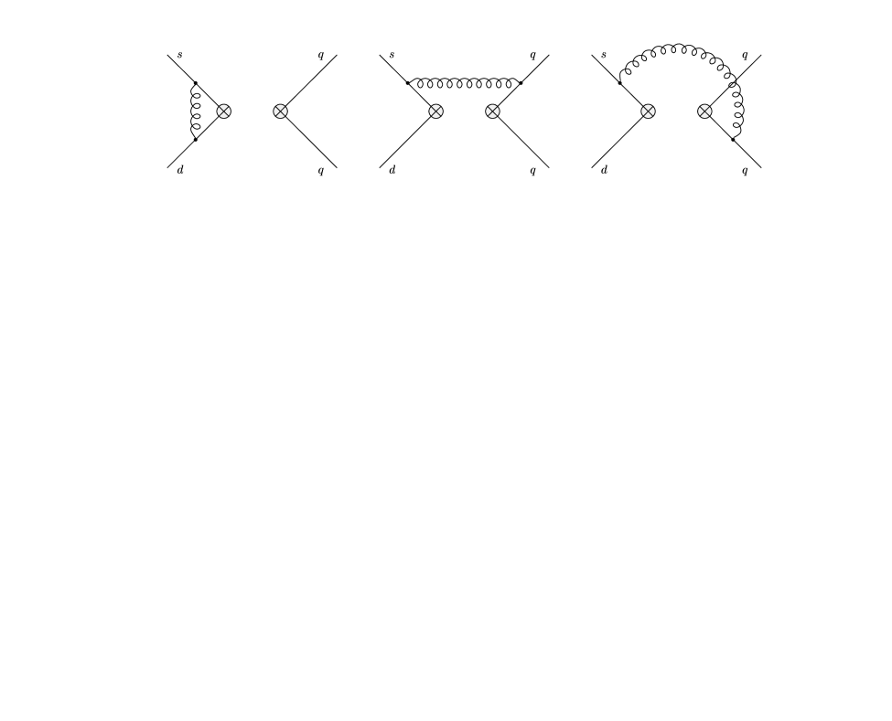
Figure 3: Diagrams contributing to the matrix element of current-current operators at ${\cal O}(\alpha_{s})$.

After renormalization in the NDR scheme, we obtain

$$\langle{\cal O}_{\!LL}(\mu)\rangle_{\rm 1loop} = \langle{\cal O}_{\!LL}\rangle_{\rm tree}+\frac{\alpha_{s}(\mu)}{4\pi}\sum_{k}\!\left[C_{F}\,\hat{1}\!\otimes\!\hat{1}\,{\cal{A}}^{(1)}_{k}(\mu)+T^{a}\!\otimes\!T^{a}{\cal{A}}^{(8)}_{k}(\mu)\right]\,T_{k}\,,\hskip 14.22636pt$$ (5.13)

$$\langle{\cal O}_{\!LR}(\mu)\rangle_{\rm 1loop} = \langle{\cal O}_{\!LR}\rangle_{\rm tree}+\frac{\alpha_{s}(\mu)}{4\pi}\sum_{k}\!\left[C_{F}\,\hat{1}\!\otimes\!\hat{1}\,{\cal{B}}^{(1)}_{k}(\mu)+T^{a}\!\otimes\!T^{a}{\cal{B}}^{(8)}_{k}(\mu)\right]\,T_{k}\hskip 14.22636pt$$ (5.14)

with $k=LL,LR,1,2,3$. The coefficients ${\cal{A}}_{k}$ and ${\cal{B}}_{k}$ which do not vanish are given by

$${\cal{A}}^{(1)}_{LL}(\mu) = -3-2\,\xi\ln x_{q}+2\,\xi\ln x_{\mu}\,,$$

$${\cal{A}}^{(8)}_{LL}(\mu) = -5+6\ln x_{q}-6\ln x_{\mu}\,,$$ (5.15)

$${\cal{A}}^{(8)}_{1}(\mu) = -{\cal{A}}^{(8)}_{2}(\mu)=-2\,{\cal{A}}^{(1)}_{3}(\mu)\ =\ -(3+\xi),$$

$${\cal{B}}^{(1)}_{LR}(\mu) = -3-2\,\xi\ln x_{q}+2\,\xi\ln x_{\mu}\,,$$

$${\cal{B}}^{(8)}_{LR}(\mu) = -7-6\ln x_{q}+6\ln x_{\mu}\,,$$ (5.16)

$${\cal{B}}^{(8)}_{1}(\mu) = {\cal{B}}^{(8)}_{2}(\mu)\ =\ -2\,{\cal{B}}^{(1)}_{3}(\mu)\ =\ -(3+\xi)\,.$$

The results for ${\cal{A}}_{k}$ can be also obtained from [17], after taking the limit $m_{s}=m_{d}=m$.

Unlike the full theory results, (5)-(5.16) are scheme dependent. For instance the constant terms depend on the way $\gamma_{5}$ is defined in $n$ dimensions — in our case they are specific to the NDR scheme. The scheme dependence is generated in the calculation of the matrix elements in the effective theory: for example, in the Dimensional Reduction (DRED) scheme [27, 28] there is no constant part in ${\cal{A}}^{(i)}_{k}$ and ${\cal{B}}^{(i)}_{k}$ but only logarithms. In the ’t Hooft-Veltman (HV) scheme [29], the constants in ${\cal{A}}^{(1,8)}_{LL}(\mu)$ are (1, $-1$) instead of $(-3,-5)$, respectively, and in ${\cal{B}}^{(1,8)}_{LR}(\mu)$ they are (1, 5) instead of $(-3,-7)$ (see also (3.9)-(3.10) of [26]). (5)-(5.16) also depend on the definition of the evanescent operators [30, 31]. It is crucial that this definition follows the one adopted in the calculation of the two-loop ${\cal O}(\alpha_{s}^{2})$ anomalous dimension matrix [26, 15]. In practice, in our case this means that we have to perform the projection on $T_{k}$ by taking traces in $n$ dimensions with anticommuting $\gamma_{5}$. As a consequence of our choice of IR regularization, and in contrast to [8, 32], this is the only occurrence of the evanescent operators in our calculation.

We have now all ingredients needed to match full and effective theories. Taking into account (5.10), (5.13) and (5.14), we see that the color-octet part of the effective Hamiltonian can be written as

$${\cal H}_{\rm eff}^{Z,8} = \frac{G_{F}}{\sqrt{2}}\frac{\alpha_{\scriptscriptstyle W}}{\pi}\frac{\alpha_{s}}{4\pi}\lambda_{t}\,T^{a}\otimes T^{a}\!\!\!\!\sum_{q=u,d,s,c,b}\!\Big{\{}\left(T_{3}^{q}-e_{q}\,s^{2}_{\scriptscriptstyle W}\right)G\,{\cal O}_{LL}+\,e_{q}\,s^{2}_{\scriptscriptstyle W}H\,{\cal O}_{LR}\Big{\}},$$ (5.17)

where the coefficients $G$ and $H$ are given by

$$G \equiv {\cal{Z}}(x_{t},x_{z},s_{\scriptscriptstyle W})+5\,C_{0}(x_{t})+6\,C_{0}(x_{t})\ln x_{\mu_{W}}\,,$$ (5.18)

$$H \equiv {\cal{Z}}(x_{t},x_{z},s_{\scriptscriptstyle W})-7\,C_{0}(x_{t})+6\,C_{0}(x_{t})\ln x_{\mu_{\scriptscriptstyle W}}$$ (5.19)

and we have introduced $x_{\mu_{W}}=\mu_{\scriptscriptstyle W}^{2}/M_{\scriptscriptstyle W}^{2}$. The unphysical and $\xi$-dependent terms obtained from the two-loop calculation of (5.10) have been canceled by analogous terms from the effective theory. Note that the scale $\mu_{\scriptscriptstyle W}$ in (5.18)-(5.19) is the scale at which the matching is performed. The scale $\mu_{\scriptscriptstyle W}$ is not related to the top quark mass renormalization scale $\mu_{t}$ appearing in (5.3) although they can be set equal. We will, however, keep them distinct in the following. Taking advantage of the identity $T_{3}^{q}=e_{q}-1/6$ and using

$$T^{a}\otimes T^{a}=\frac{1}{2}\left(\tilde{1}\otimes\tilde{1}-\frac{1}{N}\hat{1}\otimes\hat{1}\right)\,,$$ (5.20)

where $\tilde{1}$ indicates twisted color indices – like in $Q_{4}$ of (2.3) – we can rewrite (5.17) in terms of the $Q_{i}$ operators:

$${\cal H}_{\rm eff}^{Z,8}=\frac{G_{F}}{\sqrt{2}}\frac{\alpha_{\scriptscriptstyle W}}{36\pi}\frac{\alpha_{s}}{4\pi}\,\lambda_{t}\left[G\left(Q_{3}-3\,Q_{4}\right)-4\,s^{2}_{\scriptscriptstyle W}H\left(Q_{7}-3\,Q_{8}\right)-4\,c^{2}_{\scriptscriptstyle W}\,G\left(Q_{9}-3\,Q_{10}\right)\right].$$ (5.21)

From here one can read the contributions of this class of diagrams to the various Wilson coefficients at the matching scale $\mu_{\scriptscriptstyle W}$ calculated for $\xi_{\scriptscriptstyle W}=1$ in the NDR scheme.

As we have seen above, at the one-loop level and in the case of the color-singlet ${\cal O}(\alpha_{s})$ corrections the dependence on $\sin^{2}\theta_{W}$ drops out in the functions $C_{0,1}(x_{t})$. This is a consequence of the Ward identity which ensures that the photon exchange diagram has no $1/q^{2}$ pole, and it is guaranteed because the momentum carried by the $Z^{0}$ boson is vanishingly small. In the case of the octet contributions the Ward identity does not hold, because the momentum carried by the $Z^{0}$ is not small. Indeed, we verify that the $\sin^{2}\theta_{W}$-dependence is not removed from the Wilson coefficient and that the function ${\cal{Z}}$ can be decomposed into

$${\cal{Z}}(x_{t},x_{z},s_{\scriptscriptstyle W})={\cal{Z}}_{0}(x_{t},x_{z})+s^{2}_{\scriptscriptstyle W}\,{\cal{Z}}_{1}(x_{t},x_{z}).$$ (5.22)

The coefficients ${\cal{Z}}_{0,1}$ are complicated functions of $x_{t}$ and $x_{z}$ and are given in (Appendix) and (Appendix) of the Appendix. As $m_{t}$ and $M_{\scriptscriptstyle W}$ are now accurately determined, ${\cal{Z}}_{0,1}$ can be linearized in the vicinity of their central values. Using the latest experimental results $m_{t}(m_{t})=166\pm 5$ GeV, $M_{\scriptscriptstyle W}=80.394\pm 0.042$ GeV, and $M_{\scriptscriptstyle Z}=91.1867$ GeV [33], we find

$${\cal Z}_{0} = +5.1795+0.038\,(m_{t}-166)+0.015\,(M_{\scriptscriptstyle W}-80.394),$$

$${\cal Z}_{1} = -2.1095+0.0067\,(m_{t}-166)+0.026\,(M_{\scriptscriptstyle W}-80.394)$$ (5.23)

which reproduce the analytic expressions to great accuracy, better than 0.1%, within 2$\sigma$ from the central values.

It is also interesting to see how the HTE approximates these two functions. In this respect we stress that, although $G$ and $H$ are $\xi_{\scriptscriptstyle W}$-dependent quantities, their leading HTE term is gauge-independent, as $Z^{0}$-penguins are the only source of contributions quadratic in $m_{t}$. The contributions quadratic in $m_{t}$ are

$${\cal{Z}}_{0}^{HTE}=\frac{3}{4}\,x_{t}\left(1-\ln x_{z}\right)\,,\hskip 28.45274pt{\cal{Z}}_{1}^{HTE}=0$$ (5.24)

so that we find ${\cal{Z}}_{0}^{HTE}=2.39$ and ${\cal{Z}}_{1}^{HTE}=0$ at leading order in the HTE. At next-to-leading order in the HTE the approximation improves substantially, as we get ${\cal{Z}}_{0}=4.62$ and ${\cal{Z}}_{1}=-1.46$, relatively close to the central values of (5). Finally, we notice that the leading term of the HTE can be obtained considering only the diagrams involving Yukawa couplings of the top quark, as we have explicitly verified.

In summary, in this section we have calculated the gluonic corrections to the $Z^{0}$-penguin diagrams. The main results are (5.8) and (5.21).

6 QCD Corrections to the Electroweak Box Diagrams

The second part of our analysis concerns the electroweak box diagrams. Again, we will consider for definiteness the case of $\Delta S=1$ transitions. Although some ${\cal O}(\alpha_{s})$ results are available in the literature for the case in which all quark involved in the transition are down quarks [17, 34] and for the case of semi-leptonic transitions [7, 8, 32], the electroweak box diagrams involving both down and up quark lines require a new calculation that we describe in this section. Indeed, it is a fortuitous coincidence that at the one-loop level quark box diagrams containing either up or down quarks are described by the single function $B_{0}(x_{t})$ introduced in (2.17). As a by-product of this computation we will also be able to reproduce all the two-loop box results of [17, 34, 8, 32].

First, we need to recall some one-loop results necessary for the subsequent discussion. The one-loop amplitude for $\bar{s}+d\to\bar{q}+q$ with $q=u,c$ can be written as

$$M_{1loop}=\frac{-i}{16\pi^{2}}\frac{g^{4}}{4M_{\scriptscriptstyle W}^{2}}\sum_{i,j}\lambda^{(q)}_{i}\lambda_{j}\,{\cal{S}}^{(u)}(x_{i},x_{j}){\cal O}_{LL},$$ (6.1)

where $\lambda^{(q)}_{i}=|V_{qi}|^{2}$, $\lambda_{j}=V_{js}^{\ast}V_{jd}$ and ${\cal O}_{LL}$ has been defined in (5.6). The function ${\cal{S}}^{(u)}(x_{i},x_{j})$ describes a generic $\Delta S=1$ box with external up quarks and arbitrary internal quark masses $m_{i,j}$. Expanding it up to ${\cal O}(\epsilon)$, it reads

$${\cal{S}}^{(u)}(x_{i},x_{j})={\cal{S}}^{(u)}_{0}(x_{i},x_{j})+\epsilon\,{\cal{S}}^{(u)}_{1}(x_{i},x_{j},x_{\mu})+{\cal O}(\epsilon^{2})$$ (6.2)

with

$${\cal{S}}^{(u)}_{0}(x_{i},x_{j})\hskip 5.69054pt=\hskip 5.69054pt-\frac{16-7x_{i}x_{j}}{16(x_{i}-1)(x_{j}-1)}-\left[\frac{x_{i}^{2}(16+x_{j}(x_{i}-8))}{16(x_{i}-1)^{2}(x_{i}-x_{j})}\ln x_{i}+(x_{i}\longleftrightarrow x_{j})\right]\,,$$ (6.3)

$${\cal{S}}^{(u)}_{1}(x_{i},x_{j},x_{\mu})\hskip 5.69054pt=\hskip 5.69054pt-\frac{40-13x_{i}x_{j}}{32(x_{i}-1)(x_{j}-1)}-\Bigg{[}\frac{x_{i}^{2}(40+x_{j}(3x_{i}-16))}{32(x_{i}-1)^{2}(x_{i}-x_{j})}\ln x_{i}$$

$$\hskip 48.36958pt-\frac{x_{i}^{2}(16+x_{j}(x_{i}-8))}{32(x_{i}-1)^{2}(x_{i}-x_{j})}\ln^{2}x_{i}+(x_{i}\longleftrightarrow x_{j})\Bigg{]}+{\cal{S}}^{(\rm u)}_{0}(x_{i},x_{j})\ln x_{\mu}$$ (6.4)

and $x_{i,j}=m_{i,j}^{2}/M_{\scriptscriptstyle W}^{2}$. ${\cal{S}}^{(u)}$ depends on the $W$-field gauge and the above expressions hold in the ’t Hooft-Feynman gauge. Setting all light quark masses to zero and using the unitarity of the CKM matrix, the only relevant combination in the limit $\epsilon\to 0$ is

$${\cal{S}}^{(u)}(x_{t},0)-{\cal{S}}^{(u)}(0,0)=-4\,B_{0}(x_{t})\,,$$ (6.5)

where $B_{0}(x_{t})$ is the Inami-Lim function of (2.17). Taking advantage of the identity $\sum_{q=u,c}{\cal O}_{LL}=\frac{1}{3}Q_{3}+\frac{2}{3}Q_{9}$, we obtain the effective Hamiltonian induced by the box diagrams with isospin $T_{3}=1/2$ (up) quarks:

$${\cal H}_{\rm eff}(T_{3}=1/2)=-{G_{F}\over\sqrt{2}}\frac{2\alpha_{\scriptscriptstyle W}}{3\pi}\lambda_{t}\,B_{0}(x_{t})\left(Q_{3}+2\,Q_{9}\right)\,.$$ (6.6)

The case of the down-quark box diagrams is slightly more complicated in that there is a mismatch in the CKM factor between the $q=d,s$ and $q=b$ cases. This implies the introduction of two additional operators $Q_{11,12}$ [35]

$$Q_{11}=(\bar{s}d)_{V-A}\;(\bar{b}b)_{V-A}\,,\hskip 28.45274ptQ_{12}=(\bar{s}b)_{V-A}\;(\bar{b}d)_{V-A}\,.$$ (6.7)

Calling ${\cal{S}}^{(d)}(x_{i},x_{j})$ the box function for the down-quark box diagrams, we find after GIM

$$M_{1loop}^{(d,s)}=\frac{-i}{16\pi^{2}}\frac{g^{4}}{2M_{\scriptscriptstyle W}^{2}}\Big{\{}\lambda_{t}\left[{\cal{S}}^{(\rm d)}(x_{t},0)-{\cal{S}}^{(\rm d)}(0,0)\right]\Big{\}}\;{\cal O}_{LL}\,,$$ (6.8)

where we have dropped a term suppressed by $\lambda^{(d,s)}_{t}$. On the other hand, in the case of $b$ quarks $\lambda^{(b)}_{t}$ is not a suppression factor and we obtain in this case

$$M_{1loop}^{(b)}=\frac{-i}{16\pi^{2}}\frac{g^{4}}{4M_{\scriptscriptstyle W}^{2}}\Big{\{}\lambda_{t}\left[{\cal{S}}^{(d)}(x_{t},0)-{\cal{S}}^{(d)}(0,0)\right]{\cal O}_{LL}\hskip 165.02606pt$$

$$+\;\lambda^{(b)}_{t}\lambda_{t}\left[{\cal{S}}^{(d)}(x_{t},x_{t})-2\,{\cal{S}}^{(d)}(x_{t},0)+{\cal{S}}^{(d)}(0,0)\right]\big{(}Q_{11}+Q_{12}\big{)}\Big{\}}\,,\hskip 14.22636pt$$ (6.9)

The function ${\cal{S}}^{(d)}(x_{i},x_{j})$ undergoes the same decomposition of (6.2). In the ’t Hooft-Feynman gauge the coefficients take the form

$${\cal{S}}^{(d)}_{0}(x_{i},x_{j})=\frac{4-7x_{i}x_{j}}{16(x_{i}-1)(x_{j}-1)}+\left[\frac{x_{i}^{2}(4+x_{j}(x_{i}-8))}{16(x_{i}-1)^{2}(x_{i}-x_{j})}\ln x_{i}+(x_{i}\longleftrightarrow x_{j})\right]\,,$$ (6.10)

$${\cal{S}}^{(d)}_{1}(x_{i},x_{j},x_{\mu})=-\frac{4+13x_{i}x_{j}}{32(x_{i}-1)(x_{j}-1)}+\Bigg{[}\frac{x_{i}^{2}(-4+x_{j}(3x_{i}-16))}{32(x_{i}-1)^{2}(x_{i}-x_{j})}\ln x_{i}$$

$$\hskip 31.2982pt-\frac{x_{i}^{2}(4+x_{j}(x_{i}-8))}{32(x_{i}-1)^{2}(x_{i}-x_{j})}\ln^{2}x_{i}+(x_{i}\longleftrightarrow x_{j})\Bigg{]}+{\cal{S}}^{(d)}_{0}(x_{i},x_{j})\ln x_{\mu}\,.$$ (6.11)

In $n=4$ dimensions the combinations present in (6.8) and (6) reduce to

$${\cal{S}}^{(d)}(x_{t},0)-{\cal{S}}^{(d)}(0,0)=B_{0}(x_{t})$$ (6.12)

and

$${\cal{S}}^{(d)}(x_{t},x_{t})-2{\cal{S}}^{(d)}(x_{t},0)+{\cal{S}}^{(d)}(0,0)\equiv{1\over 4}S_{0}(x_{t})=\frac{1}{4}\!\left[\frac{4x_{t}\!-\!11x_{t}^{2}\!+\!x_{t}^{3}}{4(1\!-\!x_{t})^{2}}\!-\!\frac{3x_{t}^{2}\ln x_{t}}{2(1\!-\!x_{t})^{3}}\right],\hskip 14.22636pt$$ (6.13)

where $S_{0}(x_{t})$ is the box function characteristic of $\Delta F=2$ transitions. We see from (6.5) and (6.12) that $T_{3}=1/2$ and $T_{3}=-1/2$ box diagrams involve the same function $B_{0}(x_{t})$. This is true only in $n=4$ dimensions and for the ’t Hooft-Feynman gauge. We will see in the following that there is no such relation at ${\cal O}(\alpha_{s})$.

Using the identity $\sum_{q=d,s,b}{\cal O}_{LL}=\frac{2}{3}(Q_{3}-Q_{9})$, we can write the contribution to the effective Hamiltonian as

$${\cal H}_{\rm eff}(T_{3}=-1/2)={G_{F}\over\sqrt{2}}\frac{\alpha_{\scriptscriptstyle W}}{2\pi}\lambda_{t}\Bigg{\{}\frac{2}{3}B_{0}(x_{t})\left(Q_{3}-Q_{9}\right)+\frac{1}{4}\lambda^{(b)}_{t}\,S_{0}(x_{t})\left(Q_{11}+Q_{12}\right)\Bigg{\}}.$$ (6.14)

The role of the operators $Q_{11,12}$ in the RGE evolution of the Wilson coefficients between $M_{\scriptscriptstyle W}$ and $m_{b}$ has been analyzed in [35]. In the case of $\varepsilon^{\prime}/\varepsilon$, for instance, they can be safely neglected. Their ${\cal O}(\alpha_{s})$ corrections are likely to be irrelevant and will not be considered in the following.

Figure 4: Feynman graphs contributing to the ${\cal O}(\alpha_{s})$ corrections to the electroweak box diagrams. Mirror diagrams are not displayed.

We are now in the position to present the calculation of the gluonic corrections to the one-loop electroweak box diagrams. The relevant diagrams for the case of isospin $T_{3}=1/2$ are shown in Fig. 4. Both color-singlet (c), (d), (g) and color-octet (a), (b), (e), (f) diagrams are present. The calculation proceeds along the same lines as the one of Section 5. Diagrams (e), (f) and (g) present IR divergences which are regulated in the way described in the previous section. The origin and the treatment of the UV divergences, however, is fundamentally different: diagrams (c), (d) have subdivergences related to the quark-gluon interactions and are renormalized in the $\overline{\mbox{MS}}$ scheme. In fact, it is sufficient to renormalize the internal quark masses and to implement the wave function renormalization of the external legs. Of course, in the counterterm diagrams the ${\cal O}(\epsilon)$ parts of (6) and (6) have to be retained. The renormalized amplitude for the process $\bar{s}+d\to\bar{q}+q$ with $q=u,c$ can be written as

$$M_{2loop}^{box}=\frac{-i}{(16\pi^{2})^{2}}\frac{g_{s}^{2}g^{4}}{4M_{\scriptscriptstyle W}^{2}}\sum_{i,j}\lambda^{(q)}_{i}\lambda_{j}\;\sum_{k}\left[C_{F}\,\hat{1}\otimes\hat{1}\,{\cal{V}}^{\,({u},\,1)}_{k}+T^{a}\otimes T^{a}\,{\cal{V}}^{\,(u,\,8)}_{k}\right]T_{k}$$ (6.15)

with $k=LL,1,2,3$. $N$ is the number of colors and $C_{F}=(N^{2}-1)/2N$. The spinor structures $T_{k}$ have been introduced in (5). Setting $\xi_{\scriptscriptstyle W}=1$, keeping the gluon gauge parameter $\xi$ arbitrary, and without making assumptions on the masses of the internal quarks, we find

$${\cal{V}}^{\,({u},\,1)}_{LL}(x_{i},x_{j}) = {\cal{L}}^{\,({u},\,1)}(x_{i},x_{j})-2\,\xi\ln x_{q}\,{\cal{S}}^{(u)}_{0}(x_{i},x_{j})$$

$$+2\,\xi\ln x_{\mu}\,{\cal{S}}^{(u)}_{0}(x_{i},x_{j})+6\ln x_{\mu}\left(x_{i}\frac{\partial}{\partial x_{i}}+x_{j}\frac{\partial}{\partial x_{j}}\right){\cal{S}}^{(u)}_{0}(x_{i},x_{j})\,,\hskip 28.45274pt$$

$${\cal{V}}^{\,({u},\,8)}_{LL}(x_{i},x_{j}) = {\cal{L}}^{\,({u},\,8)}(x_{i},x_{j})+6\ln x_{q}\,{\cal{S}}^{(u)}_{0}(x_{i},x_{j})\,,$$ (6.17)

$${\cal{V}}^{\,({u},\,8)}_{1}(x_{i},x_{j}) = -{\cal{V}}^{\,({u},\,8)}_{2}(x_{i},x_{j})=-2\,{\cal{V}}^{\,({u},\,1)}_{3}(x_{i},x_{j})=-(3+\xi)\,{\cal{S}}^{(u)}_{0}(x_{i},x_{j})\,.$$ (6.18)

All remaining ${\cal{V}}_{k}^{(u,i)}$ vanish. The two terms in the second line of (6) describe the scale dependence introduced by the $\overline{\mbox{MS}}$ renormalization of the external fields and of the internal masses, respectively. The functions ${\cal{L}}^{(u,i)}$ are independent of the gluon gauge. The complete expressions are quite long and can be found in [36].

Concerning the effective theory, only the insertion of the operator ${\cal O}_{LL}$ is relevant in this case and the results can be found in the previous section. It is easy to verify that all the unphysical spinor structures and the gauge-dependent terms of (6)-(6.18) cancel in the matching and we are left only with contributions proportional to $T_{LL}$. Using the unitarity of the CKM matrix and (5.20), the matching of full and effective theory leads to the following contribution to the effective Hamiltonian

$$\Delta\,{\cal H}_{\rm eff}(T_{3}=1/2)={G_{F}\over\sqrt{2}}\frac{\alpha_{\scriptscriptstyle W}}{6\pi}\frac{\alpha_{s}}{4\pi}\lambda_{t}\left[B^{u}_{1}(x_{t})\left(Q_{3}+2\,Q_{9}\right)+\widetilde{B}^{u}_{1}(x_{t})\left(Q_{4}+2\,Q_{10}\right)\right].$$ (6.19)

The functions $B^{u}_{1}(x_{t})$ and $\widetilde{B}^{u}_{1}(x_{t})$ are given by

$$B^{u}_{1}(x_{t}) = -\frac{2x_{t}(23+9x_{t})}{3(x_{t}-1)^{2}}-\frac{16x_{t}(1-5x_{t})}{3(x_{t}-1)^{3}}\ln x_{t}-\frac{x_{t}(9+23x_{t})}{2(x_{t}-1)^{3}}\ln^{2}x_{t}$$

$$-\frac{6x_{t}}{(x_{t}-1)^{2}}\mbox{Li}_{2}(1-x_{t})-\frac{38}{3}B_{0}(x_{t})+4B_{0}(x_{t})\ln x_{\mu_{W}}-32x_{t}\frac{\partial B_{0}(x_{t})}{\partial x_{t}}\,\ln x_{\mu_{t}},$$

$$\widetilde{B}^{u}_{1}(x_{t}) = -\frac{6x_{t}}{x_{t}-1}-\frac{3x_{t}}{2(x_{t}-1)^{2}}\ln^{2}x_{t}-\frac{6x_{t}}{(x_{t}-1)^{2}}\mbox{Li}_{2}(1-x_{t})$$ (6.21)

$$-10\,B_{0}(x_{t})-12\,B_{0}(x_{t})\ln x_{\mu_{W}}\,.$$

Again, these results hold in the ’t Hooft-Feynman gauge $\xi_{\scriptscriptstyle W}=1$ and are specific to the NDR scheme. As we will discuss in more detail later, the scheme dependence resides in the coefficients $-38/3$ and $-10$ that multiply $B_{0}(x_{t})$. Notice also that $B^{u}_{1}$ depends on both $\mu_{t}$ and $\mu_{\scriptscriptstyle W}$.

We now consider the case of $T_{3}=-1/2$ box diagrams. The relevant two-loop diagrams are the analogue of the ones shown in Fig. 4, although in this case one should also consider the Fierz rotated diagrams, which just lead to an overall factor of 2. The renormalized amplitude can therefore be written in the same way as in (6.15), but it is characterized by new coefficients ${\cal{V}}^{(d,i)}$. These coefficients agree with the expressions given in the Appendix of [17]. After the matching with the effective theory and the implementation of the GIM mechanism, we can express the contribution to the effective Hamiltonian of the weak isospin $T_{3}=-1/2$ box diagrams as

$$\Delta\,{\cal H}_{\rm eff}(T_{3}=-1/2)={G_{F}\over\sqrt{2}}\frac{\alpha_{\scriptscriptstyle W}}{3\pi}\frac{\alpha_{s}}{4\pi}\lambda_{t}\left[B^{d}_{1}(x_{t})\left(Q_{3}-Q_{9}\right)+\widetilde{B}^{d}_{1}(x_{t})\left(Q_{4}-Q_{10}\right)\right],$$ (6.22)

where the functions $B^{d}_{1}$ and $\widetilde{B}^{d}_{1}(x_{t})$ are given by

$$B^{d}_{1}(x_{t})\!\! = \!\!-\frac{8-183x_{t}+47x_{t}^{2}}{24(x_{t}-1)^{2}}-\frac{8+27x_{t}+93x_{t}^{2}}{24(x_{t}-1)^{3}}\ln x_{t}+\frac{x_{t}(27+71x_{t}-2x_{t}^{2})}{24(x_{t}-1)^{3}}\ln^{2}x_{t}$$ (6.23)

$$-\frac{2-3x_{t}-9x_{t}^{2}+x_{t}^{3}}{6x_{t}(x_{t}-1)^{2}}\mbox{Li}_{2}(1-x_{t})+\frac{2+x_{t}}{6x_{t}}\,\zeta(2)+\frac{19}{6}B_{0}(x_{t})$$

$$-B_{0}(x_{t})\ln x_{\mu_{W}}+8x_{t}\frac{\partial B_{0}(x_{t})}{\partial x_{t}}\,\ln x_{\mu_{t}}\,,$$

$$\widetilde{B}^{d}_{1}(x_{t})\!\! = \!\!-\frac{8-23x_{t}}{8(x_{t}-1)}-\frac{8-5x_{t}}{8(x_{t}-1)^{2}}\ln x_{t}+\frac{x_{t}(3+2x_{t})}{8(x_{t}-1)^{2}}\ln^{2}x_{t}-\frac{2+x_{t}}{2x_{t}}\,\zeta(2)$$ (6.24)

$$+\frac{2-3x_{t}+3x_{t}^{2}+x_{t}^{3}}{2x_{t}(x_{t}-1)^{2}}\mbox{Li}_{2}(1-x_{t})+\frac{5}{2}B_{0}(x_{t})+3B_{0}(x_{t})\,\ln x_{\mu_{W}}\,.$$

As before, the previous expressions are specific to the NDR scheme and are valid for $\xi_{\scriptscriptstyle W}=1$.

Summarizing, in this section we have calculated the NNLO contributions originated in electroweak box diagrams. The main results are reported in (6.19) and (6.22).

7 Numerical Results

In this section we summarize our results in terms of ${\cal O}(\alpha_{\scriptscriptstyle W}\alpha_{s})$ contributions to the Wilson coefficients of the electroweak penguin operators $Q_{7-10}$ and study their numerical relevance, both at the electroweak scale and at typical hadronic scales in the NDR and HV schemes. We discuss the reduction of the $\mu_{t}$-dependence in the Wilson coefficients and the issue of the renormalization scheme dependence. We conclude with a discussion of the universality of the functions $X$ and $Y$ of the Penguin-Box Expansion.

7.1 Results for the Wilson Coefficients

Let us collect the results of (5.8), (5.21), (6.19) and (6.22). Using

$$G_{0}(x_{t},x_{z}) = {\cal{Z}}_{0}(x_{t},x_{z})+5\,C_{0}(x_{t})+6\,C_{0}(x_{t})\ln x_{\mu_{W}}\,,$$ (7.1)

$$H_{0}(x_{t},x_{z}) = {\cal{Z}}_{0}(x_{t},x_{z})-7\,C_{0}(x_{t})+6\,C_{0}(x_{t})\ln x_{\mu_{\scriptscriptstyle W}}\,,$$ (7.2)

we obtain the following ${\cal O}(\alpha_{\scriptscriptstyle W}\alpha_{s})$ corrections to the Wilson coefficients of the electroweak penguin operators

$$\Delta C_{7}(\mu_{\scriptscriptstyle W}) = \frac{\alpha_{\scriptscriptstyle W}}{6\pi}\frac{\alpha_{s}}{4\pi}\left[s^{2}_{\scriptscriptstyle W}\left(4C_{1}(x_{t})+\frac{2}{3}H_{0}(x_{t},x_{z})\right)+\frac{2}{3}s^{4}_{\scriptscriptstyle W}\,{\cal{Z}}_{1}(x_{t},x_{z})\right]\,,$$ (7.3)

$$\Delta C_{8}(\mu_{\scriptscriptstyle W}) = -\frac{\alpha_{\scriptscriptstyle W}}{3\pi}\frac{\alpha_{s}}{4\pi}\Bigg{[}s^{2}_{\scriptscriptstyle W}\,H_{0}(x_{t},x_{z})+s^{4}_{\scriptscriptstyle W}\,{\cal{Z}}_{1}(x_{t},x_{z})\Bigg{]}\,,$$ (7.4)

$$\Delta C_{9}(\mu_{\scriptscriptstyle W}) = -\frac{\alpha_{\scriptscriptstyle W}}{3\pi}\frac{\alpha_{s}}{4\pi}\Bigg{[}B^{u}_{1}(x_{t})-B^{d}_{1}(x_{t})+2C_{1}(x_{t})-\frac{1}{3}G_{0}(x_{t},x_{z})$$

$$\hskip 49.79231pt-s^{2}_{\scriptscriptstyle W}\left(2C_{1}(x_{t})-\frac{1}{3}G_{0}(x_{t},x_{z})+\frac{1}{3}{\cal{Z}}_{1}(x_{t},x_{z})\right)+\frac{1}{3}\,s^{4}_{\scriptscriptstyle W}{\cal{Z}}_{1}(x_{t},x_{z})\Bigg{]}\,,$$

$$\Delta C_{10}(\mu_{\scriptscriptstyle W}) = -\frac{\alpha_{\scriptscriptstyle W}}{3\pi}\frac{\alpha_{s}}{4\pi}\Bigg{[}\widetilde{B}^{u}_{1}(x_{t})-\widetilde{B}^{d}_{1}(x_{t})+G_{0}(x_{t},x_{z})-s^{2}_{\scriptscriptstyle W}\Big{(}G_{0}(x_{t},x_{z})-{\cal{Z}}_{1}(x_{t},x_{z})\Big{)}$$ (7.6)

$$\hskip 49.79231pt-s^{4}_{\scriptscriptstyle W}\,{\cal{Z}}_{1}(x_{t},x_{z})\Bigg{]}\,.$$

As we have seen above, there are also contributions to $C_{3,4}$ which can be extracted from (5.8), (5.21), (6.19) and (6.22). However, any electroweak correction to a gluon penguin diagram would contribute at the same order. The subset of diagrams we have computed is insufficient for these coefficients. We have organized the results in (7.3)-(7.6) according to powers of $s_{\scriptscriptstyle W}$. It should be clear by now that the zeroth order coefficient is complete and gauge-invariant. The same applies to the coefficient of $s_{\scriptscriptstyle W}^{4}$, as the only missing part of our calculation — the QCD corrections to the photon penguin diagrams — is of ${\cal O}(\alpha_{\scriptscriptstyle W}s^{2}_{\scriptscriptstyle W})$ and cannot contribute to it. On the other hand, only the leading term of the HTE of the $s^{2}_{\scriptscriptstyle W}$ coefficient is complete and gauge-invariant.

As a first check of our results, we can verify that the dependence of the NLO coefficients $C_{i}$ on the matching scale $\mu_{\scriptscriptstyle W}$ and on the top mass renormalization scale $\mu_{t}$ is removed by the scale dependence of the calculated NNLO corrections, up to terms ${\cal O}(\alpha_{\scriptscriptstyle W}s^{2}_{\scriptscriptstyle W})$ originated by the missing photon-penguins. Indeed, it is straightforward to see that

$$x_{\mu_{t}}\frac{\partial}{\partial x_{\mu_{t}}}\left(\vec{C}_{e}^{(1)}(M_{\scriptscriptstyle W})+\frac{\alpha_{s}}{4\pi}\vec{C}_{es}^{(2)}(M_{\scriptscriptstyle W})\right)={\cal O}(\alpha_{s}^{2})$$ (7.7)

and similarly for the $\mu_{\scriptscriptstyle W}$ dependence. This follows from

$$x_{\mu_{t}}\frac{\partial}{\partial x_{\mu_{t}}}\vec{C}_{e}^{(1)}(M_{\scriptscriptstyle W})=-\gamma_{0}^{m}\,\frac{\alpha_{s}}{4\pi}\,x_{t}\,\frac{\partial}{\partial x_{t}}\vec{C}_{e}^{(1)}(M_{\scriptscriptstyle W})$$ (7.8)

and

$$x_{\mu_{\scriptscriptstyle W}}\frac{\partial}{\partial x_{\mu_{\scriptscriptstyle W}}}\vec{C}_{e}^{(1)}(\mu_{\scriptscriptstyle W})=-\frac{1}{2}\,\frac{\alpha_{s}}{4\pi}\,\hat{\gamma}^{(0)^{T}}\,\vec{C}_{e}^{(1)}(\mu_{\scriptscriptstyle W}).$$ (7.9)

Here $\gamma_{0}^{m}=8$ and $\hat{\gamma}^{(0)}$ are the LO anomalous dimension of the top mass and the LO anomalous dimension matrix of the operators $Q_{i}$. Additional $\mu_{\scriptscriptstyle W}$ dependent contributions of ${\cal O}(\alpha_{\scriptscriptstyle W}\alpha_{s}s^{2}_{\scriptscriptstyle W})$ come from the QED induced mixing between the gluon and electroweak penguin operators.

The numerical values of the Wilson coefficients at the electroweak scale are reported in Table 1, where we compare the NLO and NNLO results. In all numerical calculations we employ $M_{\scriptscriptstyle W}=80.394$ GeV, $M_{\scriptscriptstyle Z}=91.1867$ GeV, and $\alpha_{s}(M_{\scriptscriptstyle W})=0.121$ [33]. In Table 1 we furthermore fix $\mu_{\scriptscriptstyle W}=\mu_{t}=M_{\scriptscriptstyle W}$, and consequently adopt $m_{t}(M_{\scriptscriptstyle W})=175.5$ GeV, which follows from the experimental value of the pole top mass, $m_{t}=174.3\pm 5.1$ GeV. For the electroweak mixing angle we use $s^{2}_{\scriptscriptstyle W}=\sin^{2}\hat{\theta}_{\overline{\rm MS}}(M_{\scriptscriptstyle Z})\simeq 0.23145$ [33, 37].

$$\begin{array}[]{|c|r|r|r|r|r|r|}\hline\cr C_{i}(M_{\scriptscriptstyle W})&{\rm NLO}_{\rm NDR}&{\rm NNLO}^{(1)}_{\rm NDR}&{\rm NNLO}^{(2)}_{\rm NDR}&{\rm NNLO}^{\rm HTE}_{\rm NDR}&{\rm NLO}_{\rm HV}&{\rm NNLO}^{(2)}_{\rm HV}\\ \hline\cr\hline\cr C_{7}(M_{\scriptscriptstyle W})&0.135&0.115&0.116&0.114&0.158&0.142\\ \hline\cr C_{8}(M_{\scriptscriptstyle W})&0&0.001&0.002&0.002&0&-0.005\\ \hline\cr C_{9}(M_{\scriptscriptstyle W})&-1.091&-1.004&-1.002&-1.014&-1.067&-0.963\\ \hline\cr C_{10}(M_{\scriptscriptstyle W})&0&-0.019&-0.024&-0.019&0&-0.003\\ \hline\cr\end{array}$$

Table 1: Wilson coefficients of the electroweak penguin operators at the scale $M_{\scriptscriptstyle W}$ in units $\alpha$ in the NDR scheme and HV schemes (see text).

We give three different values for the NNLO coefficients in the NDR scheme: ${\rm NNLO}^{(1)}$ corresponds to the expressions given in (7.3)-(7.6), which, as mentioned above, contain some gauge-dependent terms calculated in the $\xi_{\scriptscriptstyle W}=1$ gauge. In ${\rm NNLO}^{(2)}$, instead, we expand the $s^{2}_{\scriptscriptstyle W}$ coefficients of (7.3)-(7.6) in inverse powers of $m_{t}$ and retain only the leading HTE component. To this end we recall that

$$C_{1}^{\rm HTE}(x_{t})=x_{t}\left(\frac{4}{3}-\zeta(2)+\ln x_{\mu_{t}}-\ln x_{t}\right).$$ (7.10)

The formulation ${\rm NNLO}^{(2)}$ is strictly gauge-independent. The QCD corrections modify $C_{7,9}(M_{\scriptscriptstyle W})$ by about $-15\%$ and $+8\%$, respectively. The difference between ${\rm NNLO}^{(1)}$ and ${\rm NNLO}^{(2)}$ is very small, which is consistent with our expectations about the contributions of the QCD corrected photon penguin diagrams. The inclusion of a recent result for the color-singlet photon penguin contribution [13] would change the results for $C_{7}(M_{\scriptscriptstyle W})$ very little (by about $+3\%$) and marginally ($-0.4\%$) for $C_{9}(M_{\scriptscriptstyle W})$. Following Section 3, we will not include it here. Finally, the fourth column of Table 1 gives $C_{7-10}(M_{\scriptscriptstyle W})$ in the NDR scheme for the case in which all ${\cal O}(\alpha_{s})$ corrections are calculated at leading order in the HTE, ${\rm NNLO}^{\rm HTE}$. The agreement with the third column is relatively good also in this case. We also observe that in the $\xi_{\scriptscriptstyle W}=1$ gauge and at $\mu_{t}=M_{\scriptscriptstyle W}$ the dominant NNLO contribution to $\Delta C_{7-10}$ is provided by $C_{1}(x_{t})$, the color-singlet corrections to the $Z^{0}$-penguin diagrams.

The QCD corrections of (7.3)-(7.6) are specific to the NDR scheme. Using the results given in Section 5, it is not difficult to find the expressions for the Wilson coefficients of (7.3)-(7.6) in the HV scheme: the cofactors of $C_{0}(x_{t})$ in (7.1), (7.2) become (1,5) instead of (5,-7) in NDR; the cofactors of $B_{0}$ in $B^{u}_{1}$ and $\widetilde{B}^{u}_{1}$ in (6), (6.21) are (6,$-2$) instead of ($-38/3,-10$); the cofactors of $B_{0}$ in $B^{d}_{1}$ and $\widetilde{B}^{d}_{1}$ in (6.23), (6.24) become $(-3/2,1/2)$ instead of ($19/6$,5/2). The numerical values of $C_{7-10}(M_{\scriptscriptstyle W})$ in the HV scheme at NLO and NNLO for $\mu_{t}=\mu_{\scriptscriptstyle W}=M_{\scriptscriptstyle W}$ are given in the last two columns of Table 1. Also in this scheme the QCD corrections to $C_{7,9}(M_{\scriptscriptstyle W})$ are ${\cal O}(10\%)$. We note finally that at NNLO $C_{8,10}(M_{\scriptscriptstyle W})$ become non-zero, but still are very small.

7.2 Reduction of the $\mu_{t}$-dependence

It is interesting to compare the $\mu_{t}$ dependence of the Wilson coefficients before and after the inclusion of the ${\cal O}(\alpha_{s})$ corrections. This is done in Figs. 5 for $C_{7}(M_{\scriptscriptstyle W})$ and $C_{9}(M_{\scriptscriptstyle W})$, where we have used the leading log expression for the running mass of the top

$$m_{t}(\mu_{t})=m_{t}(m_{t})\left[\frac{\alpha_{s}(\mu_{t})}{\alpha_{s}(m_{t})}\right]^{12\over 23}$$ (7.11)

and employed the ${\rm NNLO}^{(2)}$ expressions in the NDR scheme.

   

Figure 5: $\mu_{t}$ dependence of $C_{7}(M_{\scriptscriptstyle W})$ and $C_{9}(M_{\scriptscriptstyle W})$ at NLO and after the inclusion of the NNLO corrections for $\mu_{\scriptscriptstyle W}=M_{\scriptscriptstyle W}$ in the NDR scheme.

Despite the fact that the NNLO corrections have not been computed completely, the reduction of the scale dependence is remarkable, and is again consistent with the idea that the contributions we have calculated are the dominant ones. We also observe that the QCD corrections to $C_{7}(M_{\scriptscriptstyle W})$ and $C_{9}(M_{\scriptscriptstyle W})$ are particularly small for $\mu_{t}\approx m_{t}$. This has also been found in the case of rare semi-leptonic decays [7]. As we will discuss below this pattern does not apply to $C_{8}$ and $C_{10}$. However, in view of the fact that $C_{8}(M_{\scriptscriptstyle W})=C_{10}(M_{\scriptscriptstyle W})=0$ at NLO, we will study their $\mu_{t}$-dependence for $\mu\ll M_{\scriptscriptstyle W}$.

In practical applications it is often useful to have simple and compact formulas for the Wilson coefficients at the weak scale. For $\mu_{\scriptscriptstyle W}=M_{\scriptscriptstyle W}$ and $\mu_{t}=m_{t}$, the NDR coefficients in the NNLO⁽²⁾ formulation and in units of $\alpha$ can be written as

$$C_{7}(M_{\scriptscriptstyle W})=0.02185\,x_{t}^{1.1482}\,,\hskip 28.45274ptC_{8}(M_{\scriptscriptstyle W})=0.000718\,x_{t}^{0.661}\,,$$

$$C_{9}(M_{\scriptscriptstyle W})=-0.438\,x_{t}^{0.580}\,,\hskip 19.91684ptC_{10}(M_{\scriptscriptstyle W})=-0.004224\,x_{t}^{1.1071}\,,$$ (7.12)

which have to be compared with the NLO expressions

$$C_{7}^{\rm NLO}(M_{\scriptscriptstyle W})=0.02268\,x_{t}^{1.1423}\,,\ \ \ C_{9}^{\rm NLO}(M_{\scriptscriptstyle W})=-0.434\,x_{t}^{0.590}\,,\ \ \ C_{8,10}^{\rm NLO}(M_{\scriptscriptstyle W})=0\,.$$ (7.13)

These expressions reproduce the results of the complete formulas with an accuracy of 0.2% or better within two sigmas of the present $m_{t}$ value.

7.3 RGE Evolution and Scheme Dependence

$$\begin{array}[]{|c|r|r|r|r|}\hline\cr C_{i}&{\rm NLO_{NDR}}&{\rm NNLO_{NDR}}&{\rm NLO_{HV}}&{\rm NNLO_{HV}}\\ \hline\cr\hline\cr C_{7}(\mu_{b})&-0.002&-0.011&-0.002&-0.010\\ \hline\cr C_{8}(\mu_{b})&0.055&0.060&0.061&0.050\\ \hline\cr C_{9}(\mu_{b})&-1.336&-1.218&-1.336&-1.243\\ \hline\cr C_{10}(\mu_{b})&0.277&0.209&0.280&0.260\\ \hline\cr\hline\cr C_{7}(\mu_{K})&-0.030&-0.032&-0.028&-0.037\\ \hline\cr C_{8}(\mu_{K})&0.142&0.160&0.151&0.135\\ \hline\cr C_{9}(\mu_{K})&-1.538&-1.375&-1.538&-1.445\\ \hline\cr C_{10}(\mu_{K})&0.582&0.441&0.589&0.553\\ \hline\cr\end{array}$$

Table 2: Wilson coefficients of the electroweak penguin operators at typical hadronic scales $\mu_{b}=4.4$ GeV and $\mu_{K}=1.3$ GeV in units of $\alpha$ in the NDR scheme and HV schemes for $\mu_{\scriptscriptstyle W}=\mu_{t}=M_{\scriptscriptstyle W}$ (see text).

Let us now study the evolution of the coefficients down to a typical hadronic scale. The inclusion of NNLO contributions proceeds as explained in Section 3. We will consider two cases: the one of $B$ meson decays, for which we will use $\mu_{b}=4.4$ GeV and the one of $K$ meson decay, corresponding to $\mu_{K}=1.3$ GeV, as used in the analysis of $\varepsilon^{\prime}/\varepsilon$ [38]. The results for NDR and HV schemes are shown in Table 2 for $\mu_{t}=\mu_{\scriptscriptstyle W}=M_{\scriptscriptstyle W}$. We recall that part (but not all) of the scheme dependence of $C_{7-10}$ is canceled in the evolution against similar terms in the anomalous dimension matrix (see e.g. [2]). As demonstrated in detail in Section 4 the renormalization scheme dependence of $C_{7-10}(M_{\scriptscriptstyle W})$ discussed above is canceled by the first term in (4.9) stemming from the renormalization group transformation. The coefficients $\vec{C}(\mu)$ are however scheme dependent through the scheme dependence at the lower end of the RGE evolution represented by the second term in (4.9). The complete cancelation of the scheme dependence of physical amplitudes occurs only with the inclusion of the matrix elements of the operators $Q_{i}$. We employ $\alpha_{s}(M_{\scriptscriptstyle Z})=0.119$, corresponding approximately to $\Lambda^{(4)}=340$ MeV. In Table 2 the entries labeled by NLO refer to the NLO case described in Section 2. The entries identified by NNLO, instead, correspond to our approximation of the full NNLO result in the form NNLO⁽²⁾. At $\mu=4.4$ GeV the shifts due to the new contributions in the NDR scheme and for $\mu_{t}=M_{\scriptscriptstyle W}$ are about $+9\%$ for $C_{8}$, $+9\%$ for $C_{9}$, $-24\%$ for $C_{10}$. $C_{7}$ remains very small. At $\mu_{K}=1.3$ GeV the situation is similar, although the shifts are naturally more pronounced. In the case of the HV scheme the NNLO corrections to $C_{9}$ are somewhat smaller than in the NDR scheme. They are comparable for $C_{7}(\mu_{b})$ and somewhat larger for $C_{7}(\mu_{K})$. The strongest scheme dependence is observed in the case of $C_{8}$ and $C_{10}$, which is not surprising as $Q_{8}$ and $Q_{10}$ are color non-singlet operators. Whereas $C_{8}$ is enhanced in the NDR scheme, it is suppressed in the HV scheme. $C_{10}$ is suppressed in both schemes but the effect is substantial in the NDR scheme and rather small in the HV scheme.

As explained in Section  3, there are other NNLO contributions that we have neglected. Some of them are not known, but we can check the magnitude of the neglected ${\cal O}(\alpha_{\scriptscriptstyle W}\alpha_{s}s^{2}_{\scriptscriptstyle W})$ effects from the term $\alpha_{s}(M_{\scriptscriptstyle W})/(4\pi)\hat{R}^{(1)}(\mu,M_{\scriptscriptstyle W})\vec{C}_{s}^{(1)}$ in (3.15). It turns out that these effects are much smaller than the NNLO contributions we have considered and are completely negligible. We also notice that, among the NNLO contributions in (3.14), the one proportional to $\vec{C}^{(2)}_{es}$ is by far the dominant in the calculation of $C_{7}$ and $C_{9}$.

   

Figure 6: $\mu_{t}$ dependence of $C_{8}(\mu_{K})$ and $C_{10}(\mu_{K})$ at NLO and after the inclusion of the NNLO corrections for $\mu_{\scriptscriptstyle W}=M_{\scriptscriptstyle W}$ in the NDR scheme.

Fig. 6 shows the $\mu_{t}$ dependence of $C_{8}(\mu_{K})$ and $C_{10}(\mu_{K})$ at NLO and NNLO order in the NDR scheme. Again, the reduction of the dependence on the renormalization scale of the top mass is remarkable. In contrast to $C_{7}$ and $C_{9}$ the NNLO corrections to $C_{8}$ and $C_{10}$ are substantial in a large range of $\mu_{t}$ and a “naive” choice $\mu_{t}=m_{t}$ in the NLO expressions would, in particular in the case of $C_{8}$, totally misrepresent the true value of these coefficients. This peculiar behaviour of $C_{8}$ and $C_{10}$ can be traced back to the fact that $C_{8}(M_{\scriptscriptstyle W})=C_{10}(M_{\scriptscriptstyle W})=0$ at NLO.

In Table 3 we show the results for the Wilson coefficients as in Table 2 but this time choosing $\mu_{t}=m_{t}$. We observe a significant reduction of the NNLO corrections in the case of $C_{7}$ and $C_{9}$ relative to Table 2. The corrections to $C_{8}$ and $C_{10}$ in the NDR scheme increase and decrease, respectively. In the case of HV they are smaller than in Table 2 but this time $C_{10}$ is slightly enhanced. In any case the strong scheme dependence of $C_{8}$ and $C_{10}$ observed in Table 2 is also evident here.

$$\begin{array}[]{|c|r|r|r|r|}\hline\cr C_{i}&{\rm NLO_{NDR}}&{\rm NNLO_{NDR}}&{\rm NLO_{HV}}&{\rm NNLO_{HV}}\\ \hline\cr\hline\cr C_{7}(\mu_{b})&-0.009&-0.011&-0.009&-0.010\\ \hline\cr C_{8}(\mu_{b})&0.053&0.059&0.059&0.051\\ \hline\cr C_{9}(\mu_{b})&-1.249&-1.241&-1.249&-1.264\\ \hline\cr C_{10}(\mu_{b})&0.256&0.218&0.259&0.266\\ \hline\cr\hline\cr C_{7}(\mu_{K})&-0.036&-0.033&-0.034&-0.037\\ \hline\cr C_{8}(\mu_{K})&0.135&0.157&0.145&0.135\\ \hline\cr C_{9}(\mu_{K})&-1.437&-1.403&-1.437&-1.468\\ \hline\cr C_{10}(\mu_{K})&0.539&0.459&0.546&0.565\\ \hline\cr\end{array}$$

Table 3: Wilson coefficients of the electroweak penguin operators at typical hadronic scales $\mu_{b}=4.4$ GeV and $\mu_{K}=1.3$ GeV in units of $\alpha$ in the NDR scheme and HV schemes for $\mu_{\scriptscriptstyle W}=M_{\scriptscriptstyle W}$, $\mu_{t}=m_{t}$ (see text).

7.4 Scheme Dependence of $C_{8}$ and $\varepsilon^{\prime}/\varepsilon$

The strong scheme dependence of $C_{8}$ at the NNLO level is welcome. In the case of the CP-violating ratio $\varepsilon^{\prime}/\varepsilon$, the operator $Q_{8}$ is by far the most important electroweak penguin operator due to its large $\Delta I=3/2$ matrix element $\langle Q_{8}(\mu_{K})\rangle_{2}=B_{8}^{(3/2)}(\mu_{K})\langle Q_{8}(\mu_{K})\rangle_{2}^{\rm{vac}}$, where ”$\rm{vac}$” stands for the vacuum insertion approximation. The scheme dependence of $\langle Q_{8}(\mu_{K})\rangle_{2}$ resides fully in $B_{8}^{(3/2)}(\mu_{K})$. As the contribution of $Q_{8}$ is the dominant ${\cal O}(\alpha)$ contribution to $\varepsilon^{\prime}/\varepsilon$ one expects that the product $B_{8}^{(3/2)}(\mu_{K})C_{8}(\mu_{K})$ is approximately $\mu_{K}$ and renormalization scheme independent with small $\mu_{K}$ and scheme dependences to be canceled by contributions of other operators which mix with $Q_{8}$ under renormalization. This is supported by renormalization group studies [14] which also show that at the NLO level $B_{8}^{(3/2)}(\mu_{K})C_{8}(\mu_{K})$ is only weakly dependent on $\mu_{K}$ for $1\mbox{ GeV}\leq\mu_{K}\leq 2\mbox{ GeV}$.

The situation with the scheme dependence of $B_{8}^{(3/2)}(\mu_{K})C_{8}(\mu_{K})$ is different. Only by including the NNLO corrections to $C_{8}(\mu_{K})$ calculated in the present paper $B_{8}^{(3/2)}(\mu_{K})C_{8}(\mu_{K})$ turns out to be almost scheme independent, whereas a substantial scheme dependence is observed at NLO. Indeed using the results of Table 3 and $B_{8,\,\rm{HV}}^{(3/2)}\simeq 1.2\,B_{8,\,\rm{NDR}}^{(3/2)}$ [38] we find for $\mu_{K}=1.3\mbox{ GeV}$

$$\frac{B_{8,\,\rm{HV}}^{(3/2)}(\mu_{K})C_{8}^{\rm{HV}}(\mu_{K})}{B_{8,\,\rm{NDR}}^{(3/2)}(\mu_{K})C_{8}^{\rm{NDR}}(\mu_{K})}=\left\{\begin{array}[]{r@{\hspace{1cm}}l}1.29\hskip 28.45274pt&\mbox{NLO}\,,\\ 1.03\hskip 28.45274pt&\mbox{NNLO}\,.\end{array}\right.$$ (7.14)

This result can be understood by recalling that at NLO $C_{8}$ has the formal expansion ${\cal O}(\alpha/\alpha_{s})+{\cal O}(\alpha)$. Now the NLO term ${\cal O}(\alpha)$ is substantially larger than the leading term ${\cal O}(\alpha/\alpha_{s})$ mainly due to the $Z^{0}$-penguin diagrams which contribute first at the NLO level. In evaluating numerically the product $B_{8}^{(3/2)}C_{8}$ one effectively includes a term ${\cal O}(\alpha\alpha_{s})$ which originates in the product of the large ${\cal O}(\alpha)$ NLO term in $C_{8}$ and the scheme dependent ${\cal O}(\alpha_{s})$ correction in $B_{8}^{(3/2)}$. As the ${\cal O}(\alpha\alpha_{s})$ term in question is really a part of the NNLO contribution and moreover it is substantial, the resulting scheme dependence of $B_{8}^{(3/2)}C_{8}$ at NLO is large. Including the ${\cal O}(\alpha\alpha_{s})$ corrections to $C_{8}$ removes this scheme dependence to a large extent as seen in (7.14).

We would like to remark that the corresponding product $B_{6}^{(1/2)}C_{6}$ related to the dominant QCD-penguin operator in $\varepsilon^{\prime}/\varepsilon$, exhibits a much smaller scheme dependence at NLO than $B_{8}^{(3/2)}C_{8}$. In this case the ratio corresponding to (7.14) is found to be $1.08$ at NLO. This is related dominantly to the fact that the NLO contribution to $C_{6}$ is relatively small compared to the leading term in contrast to the case of $C_{8}$ as discussed above.

What is the impact of our results for $C_{8}$ on $\varepsilon^{\prime}/\varepsilon\,$? Clearly the main theoretical uncertainties in $\varepsilon^{\prime}/\varepsilon$ reside in the values of the hadronic matrix elements which are substantially larger than the renormalization scheme uncertainties just discussed. Yet our calculation of NNLO corrections allows us to reduce considerably the $\mu_{t}$ and in particular the renormalization scheme dependence in the electroweak penguin sector. However, in order to give a shift in $\varepsilon^{\prime}/\varepsilon$ due to NNLO corrections one would have to include similar corrections to QCD-penguin contributions and subdominant ${\cal O}(\alpha\alpha_{s})$ terms.

On the other hand, the inspection of Table 3 and (7.14) shows that the role of the electroweak penguins for fixed hadronic matrix elements is increased by roughly $16\%$ in the NDR scheme and decreased by roughly $7\%$ in the HV scheme compared to the NLO results. As electroweak penguins contribute negatively to $\varepsilon^{\prime}/\varepsilon$, which is dominated by a positive contribution from the QCD penguin operator $Q_{6}$, the NNLO corrections to $C_{8}$ calculated here suppress $(\varepsilon^{\prime}/\varepsilon)_{\rm{NDR}}$ and enhance $(\varepsilon^{\prime}/\varepsilon)_{\rm{HV}}$ over their NLO values. As an example taking central values of the parameters used in [38] and including NNLO corrections to $C_{7-10}(\mu_{K})$ we find

$$\varepsilon^{\prime}/\varepsilon=\left\{\begin{array}[]{r@{\hspace{1cm}}l}5.9\cdot 10^{-4}\hskip 28.45274pt&\mbox{NDR}\,,\\ 6.3\cdot 10^{-4}\hskip 28.45274pt&\mbox{HV}\,.\end{array}\right.$$ (7.15)

to be compared with $7.1\cdot 10^{-4}$ (NDR) and $6.1\cdot 10^{-4}$ (HV) at NLO. Here in contrast to [38] we have used $B_{8,\,\rm{HV}}^{(3/2)}\simeq 1.2\,B_{8,\,\rm{NDR}}^{(3/2)}$ and $B_{6,\,\rm{HV}}^{(1/2)}\simeq 1.2\,B_{6,\,\rm{NDR}}^{(1/2)}$ which results in higher HV values than obtained there. We have checked that the remaining scheme dependence resides dominantly in the QCD-penguin contributions for which NNLO corrections are unknown. For larger (smaller) $B_{8}^{(3/2)}$ at fixed $B_{6}^{(1/2)}$ the impact on $\varepsilon^{\prime}/\varepsilon$ coming from NNLO corrections to electroweak penguin contributions is larger (smaller).

7.5 Universality of the Functions $X$ and $Y$

As discussed in the Introduction, any decay amplitude can be written as a linear combination of $m_{t}$-dependent functions present in the initial conditions $C_{i}(M_{\scriptscriptstyle W})$. In the absence of QCD corrections the gauge independent set relevant for non-leptonic and semi-leptonic rare $K$ and $B$ decays is given by [5]

$$X_{0}=C_{0}-4B_{0}\,,\ \ \ \ Y_{0}=C_{0}-B_{0}\,,\ \ \ \ Z_{0}=C_{0}+\frac{1}{4}D_{0}$$ (7.16)

and $E_{0}$, with $C_{0},B_{0},D_{0}$ and $E_{0}$ entering $C_{i}(M_{\scriptscriptstyle W})$ in (2.9)–(2.15). Here we will only discuss $X_{0}$ and $Y_{0}$. In the case of semi-leptonic FCNC processes the inclusion of ${\cal O}(\alpha_{s})$ corrections to $Z^{0}$-penguin and box diagrams generalizes $X_{0}$ and $Y_{0}$ to

$$X_{\ell}(x_{t})=C_{\ell}(x_{t})-4B_{\ell}(x_{t},+1/2),\ \ \ \ Y_{\ell}(x_{t})=C_{\ell}(x_{t})-B_{\ell}(x_{t},-1/2),$$ (7.17)

where $C_{\ell}(x_{t})\equiv C(x_{t})$ is given in (5.2) and

$$B_{\ell}(x_{t},\pm 1/2)=B_{0}(x_{t})+\frac{\alpha_{s}}{4\pi}B_{1}(x_{t},\pm 1/2)$$ (7.18)

with $B_{1}(x_{t},\pm 1/2)$ given in [8, 32]. Concentrating first on the operators $Q_{3}$ and $Q_{9}$ and ${\cal O}(\alpha_{\scriptscriptstyle W})$ terms in (2.9) and (2.15), respectively, our calculation of gluonic corrections to box and $Z^{0}$-penguin diagrams provides the generalization of $X_{0}$ and $Y_{0}$ relevant for non-leptonic decays as follows

$$\Delta C_{3}(M_{\scriptscriptstyle W}) = \frac{\alpha_{\scriptscriptstyle W}}{6\pi}\left[2Y_{0}-X_{0}\right]\hskip 5.69054pt\to\hskip 5.69054pt\frac{\alpha_{\scriptscriptstyle W}}{6\pi}\left[2Y_{q}-X_{q}\right]\,,$$ (7.19)

$$\Delta C_{9}(M_{\scriptscriptstyle W}) = -\frac{\alpha_{\scriptscriptstyle W}}{6\pi}\left[2Y_{0}+2X_{0}\right]\hskip 5.69054pt\to\hskip 5.69054pt-\frac{\alpha_{\scriptscriptstyle W}}{6\pi}\left[2Y_{q}+2X_{q}\right]\,,$$ (7.20)

where

$$X_{q}(x_{t}) = X_{0}(x_{t})+\frac{\alpha_{s}}{4\pi}\left(C_{1}(x_{t})-{1\over 6}\,G(x_{t},x_{z})+B_{1}^{u}(x_{t})\right)\,,$$ (7.21)

$$Y_{q}(x_{t}) = Y_{0}(x_{t})+\frac{\alpha_{s}}{4\pi}\left(C_{1}(x_{t})-{1\over 6}\,G(x_{t},x_{z})-B_{1}^{d}(x_{t})\right).$$ (7.22)

Analogously we can write in the case of the operators $Q_{4}$ and $Q_{10}$

$$\Delta C_{4}(M_{\scriptscriptstyle W})=\frac{\alpha_{\scriptscriptstyle W}}{6\pi}\left[2\widetilde{Y}_{q}-\widetilde{X}_{q}\right],\ \ \ \ \ \ \ \ \Delta C_{10}(M_{\scriptscriptstyle W})=-\frac{\alpha_{\scriptscriptstyle W}}{6\pi}\left[2\widetilde{Y}_{q}+2\widetilde{X}_{q}\right]\,,$$ (7.23)

where

$$\widetilde{X}_{q}(x_{t})=\frac{\alpha_{s}}{4\pi}\left({1\over 2}\,G(x_{t},x_{z})+\widetilde{B}_{1}^{u}(x_{t})\right),\ \ \ \ \ \widetilde{Y}_{q}(x_{t})=\frac{\alpha_{s}}{4\pi}\left({1\over 2}\,G(x_{t},x_{z})-\widetilde{B}_{1}^{d}(x_{t})\right).$$ (7.24)

Evidently, at NNLO in non-leptonic decays more $m_{t}$-dependent functions appear than in the case of semi-leptonic FCNC processes. Moreover additional functions are necessary to describe the $m_{t}$-dependence of the coefficients $C_{7}$ and $C_{8}$ as seen in (7.3) and (7.4). Furthermore, gluon corrections to photon penguins and electroweak corrections to gluon penguins will introduce new $m_{t}$-dependent functions not present in semi-leptonic FCNC decays.

We conclude therefore that at the NNLO level in non-leptonic decays the structure of $m_{t}$-dependence is much more involved than in semi-leptonic FCNC decays. On the other hand, if we restrict our discussion to the dominant $m_{t}$-dependence residing in $C_{9}(M_{\scriptscriptstyle W})$ we can say something concrete about the violation of the universality of the $m_{t}$-dependent functions addressed briefly in the Introduction. To this end we write

$$X_{q}(x_{t}) \!\!\!\!=\!\!\!\! X_{\ell}(x_{t})\!+\!\frac{\alpha_{s}}{4\pi}\!\left[4B_{1}(x_{t},\!-1/2)\!-\!{1\over 6}G(x_{t},x_{z})\!+\!B_{1}^{u}(x_{t})\right]\equiv\eta_{q\ell}^{X}\,X_{\ell}(x_{t})\equiv\eta_{q}^{X}\,X_{0}(x_{t}),\hskip 34.14322pt$$ (7.25)

$$Y_{q}(x_{t}) \!\!\!\!=\!\!\!\! Y_{\ell}(x_{t})\!+\!\frac{\alpha_{s}}{4\pi}\!\left[B_{1}(x_{t},\!-1/2)\!-\!{1\over 6}G(x_{t},x_{z})\!-\!B_{1}^{d}(x_{t})\right]\equiv\eta_{q\ell}^{Y}\,Y_{\ell}(x_{t})\equiv\eta_{q}^{Y}\,Y_{0}(x_{t}).$$ (7.26)

Clearly, the size of the various $\eta$ factors depends on the choice of $\mu_{t}$. In Table 4 we report their values for $\mu_{t}=M_{\scriptscriptstyle W}$ and $\mu_{t}=m_{t}$ in the NDR and HV schemes. As usual, we fix $\mu_{\scriptscriptstyle W}=M_{\scriptscriptstyle W}$.

$$\begin{array}[]{|c|r|r|r|r|}\hline\cr&\vrule\lx@intercol\hfil\mu_{t}=M_{\scriptscriptstyle W}\hfil\lx@intercol\vrule\lx@intercol&\vrule\lx@intercol\hfil\mu_{t}=m_{t}\hfil\lx@intercol\vrule\lx@intercol\\ \hline\cr&{\rm NDR}&{\rm HV}&{\rm NDR}&{\rm HV}\\ \hline\cr\hline\cr\eta^{X}_{q}&0.912&0.894&0.980&0.962\\ \hline\cr\eta^{Y}_{q}&0.911&0.908&1.006&1.003\\ \hline\cr\eta^{X}_{q\ell}&0.985&0.968&0.986&0.966\\ \hline\cr\eta^{Y}_{q\ell}&0.993&0.991&0.994&0.990\\ \hline\cr\end{array}$$

Table 4: $\eta$ factors for the functions $X$ and $Y$ in different schemes and for different $\mu_{t}$.

For $\mu_{t}=M_{\scriptscriptstyle W}$ the universality of $X$ and $Y$ is broken at ${\cal O}(\alpha_{s})$ by terms which are relatively small with respect to the NNLO correction, although not negligible in the HV scheme. This follows also from our previous remark that for this choice of scale the largest contribution to $C_{9}$ comes from $C_{1}(x_{t})$, which is the same for hadronic and semi-leptonic decays. In the case of $\mu_{t}=m_{t}$, however, the ${\cal O}(\alpha_{s})$ corrections to $X,Y$ never exceed $4\%$ and $C_{1}(x_{t})$ plays no longer a dominant role. Although the universality of $X$ and $Y$ is broken by effects which are of the same order of the NNLO correction, these corrections are anyway much smaller in this case for $X$ and $Y$ than in the case $\mu_{t}=M_{\scriptscriptstyle W}$.

8 Summary

In this paper we have calculated the ${\cal O}(\alpha_{s})$ corrections to the $Z^{0}$-penguin and electroweak box diagrams relevant for non-leptonic $\Delta S=1$ and $\Delta B=1$ decays. This calculation provides the complete ${\cal O}(\alpha_{\scriptscriptstyle W}\alpha_{s})$ and ${\cal O}(\alpha_{\scriptscriptstyle W}\alpha_{s}\sin^{2}\theta_{\scriptscriptstyle W}m_{t}^{2})$ corrections to the Wilson coefficients of the electroweak penguin four quark operators relevant for non-leptonic $K$- and $B$-decays. We have given arguments supported by numerical estimates that the corrections calculated by us constitute by far the dominant part of the next-next-to-leading (NNLO) contributions to these coefficients in the renormalization group improved perturbation theory.

The main results for ${\cal O}(\alpha_{s})$ corrections to the $Z^{0}$-penguin diagrams can be found in (5.8) and (5.21). Those for the box diagrams in (6.19) and (6.22). The main results for the Wilson coefficients of the electroweak penguin operators are collected in (7.3)–(7.6). The numerical values of these coefficients are collected in Tables 1–3 and in Figs. 5 and 6.

Our main findings are as follows:

• The inclusion of NNLO corrections allows to reduce considerably the uncertainty due to the choice of the scale $\mu_{t}$ in the running top quark mass $m_{t}(\mu_{t})$ present in NLO calculations. This is illustrated in Figs. 5 and 6.

• While NNLO corrections to $C_{7}$ and $C_{9}$ are generally moderate and very small for the choice $\mu_{t}=m_{t}$, they are sizable in the case of $C_{8}$ and $C_{10}$. This is illustrated in Tables 5 and 6. In particular we observe substantial renormalization scheme dependence in $C_{8}$ and $C_{10}$, whereas the scheme dependence in $C_{7}$ and $C_{9}$ is significantly smaller.

• The strong scheme dependence of $C_{8}$ allows to cancel to a large extent the scheme dependence of the matrix element $\langle Q_{8}\rangle_{2}$ relevant for $\varepsilon^{\prime}/\varepsilon$ so that the contribution of this dominant electroweak operator to $\varepsilon^{\prime}/\varepsilon$ is nearly scheme independent. This should be contrasted with the existing NLO calculations of $\varepsilon^{\prime}/\varepsilon$ which exhibit sizeable scheme dependence in the electroweak penguin sector.

• In the case of $\Delta B=1$ decays the most important among the electroweak penguin operators is the operator $Q_{9}$. As the NNLO corrections for $\mu_{t}=m_{t}$ are in the ball park of a few percent, our results have smaller impact on non-leptonic $\Delta B=1$ decays except for the reduction of the $\mu_{t}$-dependence.

• We have also investigated the breakdown of the universality in the $m_{t}$-dependent functions $X$ and $Y$. As these functions are dominated by the contribution of the color singlet $Z^{0}$-penguin diagram which is universal, the breakdown of universality through color non-singlet $Z^{0}$-contributions and box diagrams is small as illustrated in Table 4.

Although we have seen that there are arguments suggesting that our subset of NNLO corrections is dominant, several other contributions have to be calculated in order to complete the NNLO analysis for non-leptonic decays. We have discussed this formally in Section 3. A step in this direction has been made recently in [13] where ${\cal O}(\alpha_{s}^{2})$ corrections to the initial values $C_{1-6}(M_{\scriptscriptstyle W})$ have been calculated. Yet the complete ${\cal O}(\alpha_{s})$ corrections to the photon penguin diagrams relevant for non-leptonic decays and in particular the three loop anomalous dimensions ${\cal O}(\alpha_{s}^{3})$ and ${\cal O}(\alpha\alpha_{s}^{2})$ of the set $Q_{1-10}$ are unknown. The present work and the complementary calculation in [13] constitute the first steps torwards a complete NNLO calculation of non-leptonic decays and we have demonstrated here that the NNLO corrections to the Wilson coefficients of electroweak penguin operators are of phenomenological relevance.

Acknowledgments

We are grateful to E. Franco, S. Jäger, M. Misiak, L. Silvestrini and J. Urban for interesting discussions and communications. A. J. B. would like to thank Fermilab theory group for a great hospitality during his stay in September. This work has been supported in part by the Bundesministerium für Bildung und Forschung under contract 05 HT9WOA.

Appendix

In this Appendix we report the analytic expressions for the functions ${\cal{Z}}_{0,1}(x_{t},x_{z})$ introduced in (5). They read

$${\cal{Z}}_{0}(x_{t},x_{z})=-\frac{x_{t}\left(20-20x_{t}^{2}-457x_{z}+19x_{t}x_{z}+8x_{z}^{2}\right)}{32(x_{t}-1)x_{z}}$$

$$+\frac{x_{t}\left(10x_{t}^{3}-11x_{t}^{2}x_{z}-x_{t}(30-16x_{z})+4(5-17x_{z}+x_{z}^{2})\right)}{16(x_{t}-1)^{2}x_{z}}\ln x_{t}$$

$$+\frac{x_{t}\left(10-10x_{t}^{2}-17x_{z}-x_{t}x_{z}-4x_{z}^{2}\right)}{16(x_{t}-1)x_{z}}\ln x_{z}-\frac{x_{z}\left(10x_{t}^{2}-x_{t}(4-x_{z})+8x_{z}\right)}{32(x_{t}-1)^{2}}\ln^{2}x_{t}$$

$$-\frac{1}{4}x_{z}^{2}\ln^{2}x_{z}-\left[\frac{8+12x_{t}+x_{t}^{2}}{4x_{z}}-\frac{5(x_{t}-1)^{2}(2+x_{t})}{16x_{z}^{2}}\right.$$ (A1)

$$\left.-\frac{12-3x_{t}^{3}-3x_{t}^{2}(4-x_{z})+4x_{t}(3-x_{z})+4x_{z}-x_{z}^{2}}{8(x_{t}-1)^{2}}\right]\ln x_{t}\ln x_{z}$$

$$-\left(\frac{8+12x_{t}+x_{t}^{2}}{2x_{z}}-\frac{5(x_{t}-1)^{2}(2+x_{t})}{8x_{z}^{2}}-\frac{3\left(4+8x_{t}+2x_{t}^{2}-x_{t}^{3}\right)}{4(x_{t}-1)^{2}}\right)\mbox{Li}_{2}(1-x_{t})$$

$$+\frac{(x_{z}-1)^{2}\left(5-6x_{z}-5x_{z}^{2}\right)}{4x_{z}^{2}}\,\mbox{Li}_{2}(1-x_{z})-\frac{5-16x_{z}+12x_{z}^{2}+2x_{z}^{4}}{4x_{z}^{2}}\,\zeta(2)$$

$$+\frac{x_{t}(4-x_{z})\left(88-30x_{z}-25x_{z}^{2}-2x_{t}(44-5x_{z}-6x_{z}^{2})\right)}{32(x_{t}-1)^{2}x_{z}}\,\phi\left(\frac{x_{z}}{4}\right)$$

$$+\frac{16x_{t}^{4}-x_{t}(20-x_{z})x_{z}^{2}+8x_{z}^{3}-8x_{t}^{3}(14+5x_{z})+8x_{t}^{2}(12-7x_{z}+x_{z}^{2})}{32(x_{t}-1)^{2}x_{z}}\,\phi\left(\frac{x_{z}}{4x_{t}}\right)$$

$$-\Bigg{[}\frac{22+33x_{t}-x_{t}^{2}}{16(x_{t}-1)x_{z}}-\frac{5(x_{t}-1)(2+x_{t})}{16x_{z}^{2}}+\frac{2+5x_{t}^{2}+10x_{z}+x_{t}(15+x_{z})}{16(x_{t}-1)^{2}}\Bigg{]}\Phi(x_{t},x_{z})$$

and

$${\cal{Z}}_{1}(x_{t},x_{z})=\frac{x_{t}(20-20x_{t}^{2}-265x_{z}+67x_{t}x_{z}+8x_{z}^{2})}{48(x_{t}-1)x_{z}}$$

$$-\frac{x_{t}\left(10x_{t}^{3}-15x_{t}^{2}x_{z}+4(5-7x_{z}+2x_{z}^{2})-x_{t}(30+20x_{z}+4x_{z}^{2})\right)}{24(x_{t}-1)^{2}x_{z}}\ln x_{t}$$

$$-\frac{x_{t}(10-\!10x_{t}^{2}-\!33x_{z}+\!15x_{t}x_{z}-\!4x_{z}^{2})}{24(x_{t}-1)x_{z}}\ln x_{z}+\frac{x_{z}(8-\!16x_{t}+\!2x_{t}^{2}+\!10x_{z}+7x_{t}x_{z})}{48(x_{t}-1)^{2}}\ln^{2}x_{t}$$

$$+\frac{x_{z}(4+5x_{z})}{24}\ln^{2}x_{z}+\Bigg{[}\frac{20+6x_{t}+x_{t}^{2}}{12x_{z}}-\frac{5(x_{t}-1)^{2}(2+x_{t})}{24x_{z}^{2}}$$ (A2)

$$\hskip 17.07182pt+\frac{3x_{t}^{3}+2x_{t}^{2}(12-x_{z})-x_{t}(18-16x_{z}+x_{z}^{2})-2(9+4x_{z}-x_{z}^{2})}{12(x_{t}-1)^{2}}\Bigg{]}\ln x_{t}\ln x_{z}$$

$$+\left(\frac{20+6x_{t}+x_{t}^{2}}{6x_{z}}-\frac{5(x_{t}-1)^{2}(2+x_{t})}{12x_{z}^{2}}-\frac{6+6x_{t}-8x_{t}^{2}-x_{t}^{3}}{2(x_{t}-1)^{2}}\right)\mbox{Li}_{2}(1-x_{t})$$

$$-\frac{(x_{z}-1)^{2}\left(5-10x_{z}-7x_{z}^{2}\right)}{6x_{z}^{2}}\,\mbox{Li}_{2}(1-x_{z})+\frac{10-40x_{z}+36x_{z}^{2}+4x_{z}^{3}+5x_{z}^{4}}{12x_{z}^{2}}\,\zeta(2)$$

$$+\frac{x_{t}(x_{z}-4)\left(24-26x_{z}-13x_{z}^{2}-6x_{t}(4-x_{z}-x_{z}^{2})\right)}{16(x_{t}-1)^{2}x_{z}}\,\phi\left(\frac{x_{z}}{4}\right)-\Bigg{[}\frac{2x_{t}^{2}(2+x_{t})}{3(x_{t}-1)x_{z}}$$

$$\hskip 17.07182pt-\frac{24x_{t}^{3}+12x_{t}^{2}(14+x_{z})-2x_{z}(4+5x_{z})-x_{t}(80-36x_{z}+7x_{z}^{2})}{48(x_{t}-1)^{2}}\Bigg{]}\,\phi\left(\frac{x_{z}}{4x_{t}}\right)$$

$$+\Bigg{[}\frac{10-x_{t}-x_{t}^{2}}{8(x_{t}-1)x_{z}}-\frac{5(x_{t}-1)(2+x_{t})}{24x_{z}^{2}}+\frac{6+3x_{t}^{2}+14x_{z}+5x_{t}(7+x_{z})}{24(x_{t}-1)^{2}}\Bigg{]}\,\Phi(x_{t},x_{z})\,.$$

We recall that $\zeta(2)=\pi^{2}/6$. The function $\phi(z)$ appearing in the above expressions is given by

$$\phi(z)=\left\{\begin{array}[]{ll}4\sqrt{{z\over 1-z}}~{}\mbox{Cl}_{2}(2\arcsin\sqrt{z})\,,&0<z\leq 1\,,\\ {1\over\beta}\left[-4{\rm Li_{2}}({1-\beta\over 2})+2\ln^{2}({1-\beta\over 2})-\ln^{2}(4z)+2\zeta(2)\right]\,,&z>1\,,\end{array}\right.$$ (A5)

where $\mbox{Cl}_{2}(x)={\rm Im}\,{\rm Li_{2}}(e^{ix})$ is the Clausen function and $\beta=\sqrt{1-{1/z}}$. Defining

$$\lambda(x,y)=\sqrt{(1-x-y)^{2}-4xy},$$

the function $\Phi(x,y)$ admits two different representations, according to the sign of $\lambda^{2}(x,y)$. For $\lambda^{2}\geq 0$ we have

$$\Phi(x,y)=\lambda\left\{2\ln\left(\frac{1+x-y-\lambda}{2}\right)\ln\left(\frac{1-x+y-\lambda}{2}\right)-\ln x\ln y\right.\hskip 28.45274pt$$

$$\left.-2\,\mbox{Li}_{2}\left(\frac{1+x-y-\lambda}{2}\right)-2\,\mbox{Li}_{2}\left(\frac{1-x+y-\lambda}{2}\right)+2\,\zeta(2)\right\},$$ (A6)

while for $\lambda^{2}\leq 0$

$$\Phi(x,y)=-2\,\sqrt{-\lambda^{2}}\left\{\mbox{Cl}_{2}\left[2\arccos\left(\frac{-1+x+y}{2\sqrt{xy}}\right)\right]\right.\hskip 113.81102pt$$

$$\left.+\mbox{Cl}_{2}\left[2\arccos\left(\frac{1+x-y}{2\sqrt{x}}\right)\right]+\mbox{Cl}_{2}\left[2\arccos\left(\frac{1-x+y}{2\sqrt{y}}\right)\right]\right\}.$$ (A7)

Additional details on this function can be found in [39].

References

• [1] R. Fleischer, Int. J. of Mod. Phys. A12 (1997) 2459; A.J. Buras and R. Fleischer, hep-ph/9704376, in Heavy Flavours II, World Scientific (1998), Eds. A.J. Buras and M. Lindner, p. 65.
• [2] G. Buchalla, A.J. Buras, and M.E. Lautenbacher, Rev. Mod. Phys. 68 (1996) 1125.
• [3] T. Inami and C.S. Lim, Progr. Theor. Phys. 65 (1981) 297, ibid. 65 (1981) 1772 (E).
• [4] A.J. Buras, hep-ph/9806471, in Probing the Standard Model of Particle Interactions, eds. R. Gupta, A. Morel, E. de Rafael and F. David (Elsevier Science B.V., Amsterdam, 1998), p. 281; A.J. Buras, hep-ph/9905437, Lectures given at the 14th Lake Louise Winter Institute.
• [5] G. Buchalla, A.J. Buras and M.K. Harlander, Nucl. Phys. B 349 (1991) 1.
• [6] G. Buchalla and A.J. Buras, Nucl. Phys. B398 (1993) 285.
• [7] G. Buchalla and A.J. Buras, Nucl. Phys. B400 (1993) 225.
• [8] M. Misiak and J. Urban, Phys. Lett. B451 (1999) 161.
• [9] K. Adel and Y.P. Yao, Modern Physics Letters A8 (1993) 1679; Phys. Rev. D 49 (1994) 4945.
• [10] C. Greub and T. Hurth, Phys. Rev. D 56 (1997) 2934.
• [11] A.J. Buras, A. Kwiatkowski and N. Pott, Nucl. Phys. B 517 (1998) 353.
• [12] M. Ciuchini, G. Degrassi, P. Gambino and G. F. Giudice, Nucl. Phys. B 527 (1998) 21.
• [13] C. Bobeth, M. Misiak and J. Urban, hep-ph/9910220.
• [14] A.J. Buras, M. Jamin, and M.E. Lautenbacher, Nucl. Phys. B408 (1993) 209.
• [15] M. Ciuchini, E. Franco, G. Martinelli, and L. Reina, Nucl. Phys. B415 (1994) 403.
• [16] W. Marciano and A. Sirlin, Phys. Rev. D22 (1980) 2695.
• [17] A.J. Buras, M. Jamin, and P.H. Weisz, Nucl. Phys. B347 (1990) 491.
• [18] P. Gambino, P.A. Grassi, and F. Madricardo, Phys. Lett. B454 (1999) 98.
• [19] P. Gambino, A. Kwiatkowski, and N. Pott, Nucl. Phys. B544 (1999) 532.
• [20] K. Aoki, et al., Suppl. Progr. Theor. Phys. 73 (1982) 1.
• [21] S. Wolfram, The MATHEMATICA book, 3rd edition, Wolfram Media, 1996.
• [22] J. Küblbeck, M. Böhm, and A. Denner, Comp. Phys. Commun. 60 (1991) 165; H. Eck, FeynArts 2.0—A generic Feynman diagram generator, PhD thesis, Universität Würzburg, 1995; the latest version 2.2 with updated User’s Guide by T. Hahn is available at ftp://ftp.physik.uni-wuerzburg.de/pub/hep/index.html.
• [23] M. Jamin and M.E. Lautenbacher, Comp. Phys. Commun. 74 (1993) 265.
• [24] G. Degrassi, P. Gambino, and S. Fanchiotti, ProcessDiagram, unpublished.
• [25] R. Mertig and R. Scharf, Comp. Phys. Commun. 111 (1998) 265.
• [26] A.J. Buras, M. Jamin, M.E. Lautenbacher, and P.H. Weisz, Nucl. Phys. B400 (1993) 37.
• [27] W. Siegel, Phys. Lett. B84 (1979) 193.
• [28] A.J. Buras and P.H. Weisz, Nucl. Phys. B333 (1990) 66.
• [29] G. ’t Hooft and M. Veltman, Nucl. Phys. B44 (1972) 189. P. Breitenlohner and D. Maison, Commun. Math. Phys. 52 (1977) 11,39,55.
• [30] M.J. Dugan and B. Grinstein, Phys. Lett. B256 (1991) 239.
• [31] S. Herrlich and U. Nierste, Nucl. Phys. B455 (1995) 39.
• [32] G. Buchalla and A.J. Buras, Nucl. Phys. B548 (1999) 309.
• [33] The LEP and SLD Electroweak Working Groups, preprint CERN-EP/99-15, February 1999; for the most recent preliminary results, see http://www.cern.ch/LEPEWWG.
• [34] J. Urban, et al., Nucl. Phys. B523 (1998) 40.
• [35] G. Buchalla, A.J. Buras, and M.K. Harlander, Nucl. Phys. B337 (1990) 313.
• [36] U. A. Haisch, QCD Korrekturen zu den Wilson Koeffizienten der elektroschwachen Pinguin Operatoren, Diploma thesis, TU München, 1999.
• [37] G. Degrassi, P. Gambino, and A. Sirlin, Phys. Lett. B394 (1997) 188.
• [38] S. Bosch et al., hep-ph/9904408.
• [39] A.T. Davydychev and B. Tausk, Nucl. Phys. B397 (1993) 123.