Scales and Phases of Non-Perturbative QCD

Abstract

This is a short write-up of lectures at UK Theory Institute, Swansea UK, Sept.99; and XVII School “QCD: Perturbative or Non-perturbative?” Lisbon,Portugal, Oct.99. The covered topic include (i) discussion of the scales at which perturbative description should be changed by the non-perturbative one. A number of various examples are considered, leading to different scales, related to instantons or confinement effects; (ii) Instanton vacuum as an Instanton Liquid; (iii) The phase diagram of QCD at finite temperature and density, and especially description of a recent progress in Color Superconductivity.

1 Introduction

I hardly need an explanation of why I have devoted so large portion of these lectures to such introductory subject as “scales” of non-perturbative QCD. First of all, it answers the question put in the title of the Lisbon school. The second reason: somewhat surprisingly to me, naive simplistic ideas originating in 70’s - the picture hadrons as some structureless perturbative “bags”, with very soft non-perturbative effects appearing only at its boundaries at the scale 1 fm – are still alive and well, in spite of multiple evidences to the contrary, pointed to existence of some substructures inside hadrons. The lectures in such schools is probably the right place to collect at least few simplest evidences for that in one place.

Indeed, the perturbative QCD naturally points toward the $\Lambda_{QCD}\sim 200\ MeV$, the position of the so called Landau pole, as the momentum scale where it becomes inapplicable. Since the inverse of it, 1 fm, is a typical hadronic size, such cutoff indeed seemed natural. The basic approach to non-perturbative physics which has started in 70’s, the QCD sum rules, have been based on such a picture. If the non-perturbative fields be so “soft”, the derivative expansion, known as Operator Product Expansion (OPE), should be reasonable convergent. Furthermore, smooth connection between hadronic and partonic approaches hoped to be possible.

However it was realized in 80’s that the non-perturbative fields actually form structures with sizes significantly smaller than 1 fm. Two most important non-perturbative objects are instantons (with the average size $\rho\sim 1/3fm$ [1]) and confining strings (with the radius of the gluoelectric field only about $r_{string}\approx 1/5fm$, see fig.2b ). the ratio of those to hadronic size R enters in the 4-th power for $\rho$ and in the 2-th for $r_{string}$, so in both cases only a small fraction, few percent, of hadronic volume is occupied by them. The simplest picture of it is that of constituent quarks (or, possibly, scalar diquarks as well) of the size $\sim\rho$, connected by strings.

Can we see it in some observables? The simplest thing is to monitor the onset of the non-perturbative effects at small distances/ large momenta where these phenomena just become comparable to perturbative effects, and, furthermore, the OPE expansion in derivatives start to fail. Where it happens would define the scales we speak about, as you see the number depends on a particular physical problem considered: several different situation which have been identified so far will be discussed in this section. For pedagogical reason, we do it in two rounds: at the first one (section 2) we present the “naive” predictions and, in many cases, see if those really work.

In the second round (the next sections 3,4) we discuss the explanations (to the extent they are understood today). The conclusions we draw from these observations are that in several observables already the distances $r=0.1-0.2$ used in these studies are already large enough to be outside the validity domain of the original quark-gluon description, even reinforced by the OPE corrections. Effective approaches like Interacting Instanton Liquid Model (IILM) or Abelian Higgs Model (AHM) should rather be used here, and those indeed provide at least semi-quantitative explanations of the non-perturbative effects.

One of the reasons the “naive” point of view mentioned above has survived for so long is that many applications deal with a special case of vector currents. Those are related with such long-studied reactions as the $e^{+}e^{-}\rightarrow$ hadrons and deep inelastic scattering. The QCD sum rules work well for this cases, e.g. the “next twist” correction to deep inelastic scattering are surprisingly small, etc. (We will show some of this in section 5, when we will discuss vector correlators.) However, if one looks more systematically at various channels (see e.g. review [19]), it is clear that the behavior of the vector channels is in fact a single exception. Cancellation of all corrections in this case is observed but not yet fully understood. It seems like vector currents simply cannot see these vacuum/hadronic substructure at all.

We go into more detailed discussion of the instanton-induced effects in chapter 4. It is shown there that consistent treatment of those, to all orders in ’t Hooft interaction, has been worked out. The so called Interacting Instanton Liquid Model (IILM) reproduces all correlation functions known from phenomenology (hadronic masses and coupling constants) and/or direct lattice measurements.

We continue to discuss instanton-induced effects in the last chapter 5, but now in connection with “new frontiers” in QCD leading to qualitatively new phases. Among those are Quark-Gluon Plasma (QGP) at $high$ T and high baryonic density; Color Superconductivity (CSC) at $low$ T and high baryonic density, and the Conformal Phase at larger number of flavors.

2 The Scales of Non-Perturbative QCD

2.1 The Chiral Scale

Historically the first is the so called chiral scale $\Lambda_{\chi}\sim 1\ GeV$, the upper limit of low energy effective theories such as effective chiral Lagrangians or Nambu-Jona-Lasinio model [2]. Although it does not follow that it is also the low boundary of perturbative treatment, it cannot at least be lower.

These effective theories appeared in 60’s, before QCD was even invented. Their parameters were simply fitted to observations: e.g. the first Weinberg term of the chiral Lagrangian contains 2 derivatives and the pion decay constant $f_{\pi}$, the next have 4 derivatives and the so called Leutwyler couplings, etc. The “chiral scale” appears when one asks at which momenta all terms of the chiral Lagrangian become of the same magnitude.

The NJL model is somewhat more microscopic: it does not start with the Goldstone modes (pions), but derives instead the chiral symmetry breaking and Goldstone modes starting from some hypothetical 4-fermion interaction. I would not describe this model here, and only make few comments about it. (i) It was the first bridge between theory of superconductivity and quantum field theory: in a way, it first shown that the vacuum of the of strong interaction should be truly non-perturbative. It has a non-zero quark condensate and a gap 330-400 MeV, known as “constituent quark mass”; (ii) The model has basically 2 parameters: the strength of its 4-fermion interaction G and the cutoff $\Lambda\sim.8-1GeV$. The latter regulates the loops: this model is non-renormalizable. The latter parameter can also be seen as the inverse size of the constituent quarks; (iii) The interaction on which NJL model was based is hypothetical, and we should ask now if QCD actually generates it. People have been first trying to explain the NJL forces as being due to one gluon exchange diagrams. However it became clear by now that it is not so, and the true origin of the NJL-type short-range quark-antiquark attractions comes from the instantons; (iv) The symmetries of the resulting 4-fermion effective interaction, known as ’t Hooft Lagrangian, are not the same as of the original NJL model. They explicitly break this chiral U(1) symmetry (rotating all fermions by $exp(i\phi*\gamma_{5})$), as a result of which the $SU(3)_{f}$ singlet meson $\eta^{\prime}$ is $not$ a Goldstone boson. NJL model was wrong at this point.

Instead, we rather consider another incarnation of the chiral scale, defined as the energy/momentum scale at which the non-perturbative effects become equal to perturbative ones (in fact, the zeroth order in $\alpha_{s}$) in $J^{P}=O^{\pm}$ correlation functions.

Let us consider two currents separated by space-like distance x (the spatial distance, or Euclidean time) and consider the correlation functions of the type

$$K(x)=<T(J(x)J(0))>$$ (1)

with $J(x)=\bar{\psi}(x)\Gamma\psi(x)$. The matrix $\Gamma$ contains $\gamma_{5}$ for pseudoscalar channels, and a flavor matrices, if we discuss e.g. pions. For simplicity, we will restrict ourselves in what follows to 2 quark flavors. It means we have 4 channels: $\pi$ (P=-1, I=1), $\sigma$ (P=+1,I=0), $\eta$ (P=-1,I=0) and $\delta$ (or ???) (P=+1,I=1).

In all cases at small x we expect $K(x)\approx K_{0}(x)$ where the latter corresponds to just free propagation of light quarks. If they are massless, the correlators are $K_{0}(x)=12/(\pi^{4}x^{6})$, basically the square of the massless quark propagator.

The first deviations due to non-perturbative effects have been calculated using the OPE [11], in the context of QCD sum rules. Ignoring subtleties, one can view it as just expansion in x at small x. For scalar and pseudoscalar channels the result for the first correction is

$${K(x)\over K_{0}(x)}=1+{x^{4}\over 384}<(gG)^{2}>+...$$ (2)

If the “gluon condensate” is made out of soft vacuum filed, they are are long range as compared to $x$ and therefore all their arguments can be simply taken at the point x=0. The value of the “gluon condensate” appearing here was estimated previously from charmonium sum rules:

$$<(gG)^{2}>_{SVZ}\approx.5\,GeV^{4}$$ (3)

Thus, the OPE suggests the scale at which the correction becomes equal to the first term:

$$x_{OPE}=(384/<(gG)^{2}>_{SVZ})^{1/4}\approx 1.0\,fm$$ (4)

which seems to be completely consistent with the expectations.

However, as the Novikov, Shifman, Vainshtein and Zakharov soon noticed [3], this (and other OPE corrections) had completely failed to describe all $J^{P}=O^{\pm}$ channels. It was very puzzling, because for vector and axial channels it did a good job [11]. That is why they asked an important question (the title of their paper): “Are all hadrons alike?”.

How do we know that this scale is wrong? Let us just do the simplest thing: consider the pion contribution to the correlator in question

$$K_{\pi}(x)={\lambda_{\pi}^{2}\over 4\pi^{2}x^{2}}$$ (5)

The coupling constant is defined as $\lambda_{\pi}=<0|J(0)|\pi>$ and the rest is nothing else as the scalar massless propagator. (We can ignore the pion mass at distances in question.)

Because both the pion term and the gluon condensate correction are $1/x^{2}$, let us compare the coefficients. Ideal matching would mean they are about the same:

$$\lambda_{\pi}^{2}\approx{<(gG)^{2}>_{SVZ}\over 8\pi^{2}}$$ (6)

The r.h.s. is about 0.0063 GeV⁴. However (unlike the better known coupling to the axial current $f_{\pi}$), the $\lambda_{\pi}$ is surprisingly large. The l.h.s. of this relation is actually $\lambda_{\pi}^{2}=(.48\,GeV)^{4}=0.053\,GeV^{4}$, or about 10 times larger than the r.h.s. It means some other and much larger effect should explain deviation from the perturbative behavior. Why it has not showed up in the vector channels? We return to these questions in the next section.

2.2 The Scale of the $J^{P}=O^{\pm}$ glueball correlation functions

It is defined in the same way as the first one, only for scalar and pseudoscalar glueball correlators. Instead of the quark currents we have now operators $G_{\mu\nu}^{2}$ and $G_{\mu\nu}\tilde{G}_{\mu\nu}$ (tilde means dual field in electric-magnetic sense, or convolution with $\epsilon_{\alpha\beta\gamma\delta}/2$. The analogous OPE expressions for these two channels [3] now starts with the next gluonic “condensate”

$$K_{J=\pm 1}(x)=\pm{384\over\pi^{4}x^{8}}[1\pm{\pi^{2}x^{6}\over 192}<g^{3}f^{abc}G_{\mu\nu}^{a}G_{\nu\sigma}^{b}G_{\sigma\nu}^{c}>+...]$$ (7)

Again, the first term is the free propagation of gluons, it is the largest one at small x. Note that the power of x in both terms simply follows from dimension. Demanding that these two terms are equal, we get the corresponding “OPE scale”.

However, as emphasized in this paper [3], other theoretical arguments suggested that in fact the non-perturbative physics should start at much smaller scale. One of them is based on low energy theorem

$$\int d^{4}xK_{+}(x)={128\pi^{2}\over b}<(gG)^{2}>$$ (8)

where b=${11N_{c}\over 3}-{2N_{f}\over 3}\approx 9$ is the first coefficient of the beta function.

One way to see what it means is to assume that the major deviation at small distances is due to the contribution of the scalar glueball . Then the integral can be related to the coupling constant $\lambda_{0+}=<0|G^{2}|{0+}\ glueball>$ and the glueball mass $m_{0+}$ in a simple case

$${\lambda_{0+}^{2}\over m_{0+}^{2}}={128\pi^{2}\over b}<(gG)^{2}>$$ (9)

It is known from lattice and phenomenology that $m_{0+}\approx 1.6GeV$, so we now can obtain the coupling. Then we can go back to $K_{+}(x)$ at small x and see where the glueball contribution becomes equal to the perturbative part, to define the scale.

Like in the pion case, both the OPE correction and the coupling produce $1/x^{2}$ effects at small distances, so we again compare the coefficients. The OPE-hadron matching would work if they are close

$$\lambda_{0+}^{2}\approx 8<g^{3}f^{abc}G_{\mu\nu}^{a}G_{\nu\sigma}^{b}G_{\sigma\nu}^{c}>$$ (10)

but in fact the value we infer from the low energy theorem gives 1.8 GeV⁶ for the l.h.s., which again significantly exceeds the l.h.s. (when the phenomenological value of the VEV of $G^{3}$ operator is substituted.).

More strict way [3] to say the same thing is to go to momentum representation (Fourier transform $\tilde{K}_{+}(q)$ of the correlation function. The total integral over x corresponds to the zero momentum value. Since we know it, we can subtract it in the dispersion relation

$$\tilde{K}_{+}(Q)={1\over\pi}\int ds{Im\tilde{K}_{+}(s)\over(s+Q^{2})}$$ (11)

where $Q^{2}=-q^{2}>0$. The subtraction improves the convergence of the integral at large Q of the dispersion relation, namely

$${\tilde{K}_{+}(Q)\over Q^{2}}={\tilde{K}_{+}(0)\over Q^{2}}+{1\over\pi}\int ds{Im\tilde{K}_{+}(s)\over s(s+Q^{2})}$$ (12)

This argument shows that in momentum space the effective subtraction term becomes equal to perturbative one at the momentum scale $\Lambda_{0^{\pm}glueballs}\sim(3-4)\ GeV$, the largest of the effective scales of the non-perturbative QCD Other set of arguments presented in the same paper have shown, that the same scale should appear in the pseudoscalar glueball channel as well. Why this happens in this case at much larger scale than for any quark channels?

2.3 Heavy Quarkonia and Small Size Instantons as Dynamical Dipoles

Another way of looking at the onset of non-perturbative physics is to separate color charges by some small distance, and see what happens. (The correlation functions considered above deal with two colorless operators, also separated by a small distance x.) We will call such cases generically “a small-size color dipoles”. There would be three different kinds of those.

Historically the first example are states of heavy quarkonia. The non-perturbative correction to their energies was calculated by Voloshin and Leutwyler [10] by OPE: $\delta E\sim<0|g^{2}G_{\mu\nu}^{2}|0>r^{2}\ \tau$ where the spatial size $r\sim 1/(\alpha_{s}M)$ and the rotational time $\tau\sim 1/(\alpha_{s}^{2}M)$, both small for large quark mass M. (I am not going to bother you with exact expression, in which r appears as some dipole matrix element and $\tau$ as energy denominators, as well by questions how small is $\alpha_{s}$ and what is its argument.)

The question is whether this correction is indeed what is the case in reality. The answer probably exists or can be worked out using the spectroscopic information about Upsilons at hand: unfortunately I am not aware of any precision studies of it.

Let me therefore move on to another kind of “dynamical dipoles”, the instantons, now 4-dimensionally symmetric, with $r\sim\tau\sim\rho$. One of the reason is I know it better, but there is also a more scientific explanation of why one should do it instead. Instantons in general are much more sensitive tool, because the tunneling probability contains the perturbative/semi-classic term (as well as all non-perturbative corrections) in the exponent.

(A side remark: as noticed in my paper [12], it is in particular should be very important for fixing the value of $\Lambda_{QCD}$. Experimentalists made tremendous efforts to get it from scaling violation and similar effects containing log($\Lambda_{QCD})$, but still get poor accuracy. Lattice practitioners use hadronic masses and especially splittings of some quarkonium levels for this purpose, which are effects $const*\Lambda_{QCD}$, and improved the accuracy. But the the density of small size instantons, calculated semi-classically in a seminal paper by ’t Hooft [14], contains $O(\Lambda_{QCD})^{b}$ where $b=(11N_{c}/3-2N_{f}/3)\sim 9$. So the instanton-based determination of $\Lambda_{QCD}$ should be potentially 10 times more accurate!)

Similar to Voloshin-Leutwyler correction, the OPE-based result [11] predicts the following correction to the density of instantons of size $\rho$:

$$dn(\rho)=dn_{pert}(\rho)(1+{\pi^{4}\rho^{4}\over 2g^{4}}<0|g^{2}G_{\mu\nu}^{2}|0>+...)$$ (13)

It is also second order dipole approximation: the instanton dipole is $O(\rho^{2}/g)$. Note the generic 4-th power of $\rho$ is also determined by the dimension of the lowest gauge invariant local operator. Note also the sign: it is nothing else but a generic attraction resulting from $any$ second order perturbation. However both these conclusions happen to be in apparent conflict with the lattice data (see below).

In Fig.[1](a) we show recent lattice data for the instanton size $distribution$ in pure SU(3) gauge theory [13]. (There are others but, this work includes such refinements as improved lattice action and back extrapolation to zero smoothening.) One can clearly see, that a rapid rise at small $\rho$ turns into a strong suppression. The former behavior is consistent with the semi-classical one-loop result [14]:

$${dN_{0}\over d\rho}|_{pert}={C_{N_{c}}\over\rho^{5}}({8\pi^{2}\over g^{2}(\rho)})^{2N_{c}}(\rho\Lambda)^{b}$$ (14)

where $C_{N_{c}}$ is the normalization constant, the $\rho^{-5}$ factor and the term with the coupling constant comes from the Jacobian of the zero modes, and $b=(11N_{c}/3-2N_{f}/3)$ as already mentioned.

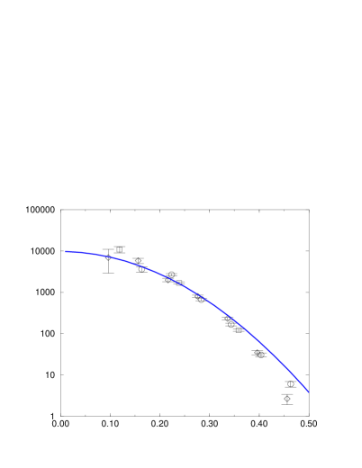
Fig. 1: (a) The instanton density $dn/d\rho d^{4}z$, [fm^-5] versus its size $\rho$ [fm]. (b) The combination $\rho^{-6}dn/d\rho d^{4}z$, in which the main one-loop behavior drops out for $N_{c}=3,N_{f}=0$. The points are from the lattice work [13], for this theory, with $\beta$=5.85 (diamonds), 6.0 (squares) and 6.1 (circles). Their comparison should demonstrate that results are rather lattice-independent. The line corresponds to the proposed expression $\sim exp(-2\pi\sigma\rho^{2})$, see text.

Sharp maximum seen in Fig.[1](a) appears at rather small $<\rho>\approx 1/3$ $fm$, much smaller that their spacing $R\approx 1$ $fm$. This results in a non-trivial “vacuum diluteness” parameter [1] to which we turn in section 5, but now we are not interested in a typical instanton size but rather in their suppression. Therefore we re-plot the same data in Fig.[1](b), with the leading semi-classical behavior taken away. Now the maximum is gone and one finds the $same$ suppression pattern at both sides of the maximum. The OPE prediction (13) is not seen: probably it is only true at $very$ small $\rho$. The suppression effect is clearly $O(\rho^{2})$, and not just for small $\rho$ but in the whole region.

Fig. 2: (a) The potential at small distances from [31], the quantity $r_{0}\approx 0.5$ fm denotes the so called Sommer scale is used in lattice works. (b) The fits of the transverse distribution of electric and magnetic fields in the string, obtained in lattice calculation, to ANO vortex solution of the AHM [9]. It leads to Higgs mass 1.3 GeV.

2.4 Small Static Dipoles

Another way to look at these issues is to use small static color dipoles, or short strings. As time scale $\tau$ is now unlimited, there is no OPE prediction like (13). However using just the second order dipole approximation [27] one gets a similar prediction of the non-perturbative corrections to the static potential

$$V(r)=-{4\alpha_{s}(r)\over 3}{1\over r}$$

$$+r^{2}\int d\tau\ e^{(-{3\alpha_{s}(r)\tau\over 2r})}<0|G_{\mu\nu}(\tau)U_{\tau}G_{\mu\nu}(0)U^{+}_{\tau}|0>)$$ (15)

where the field strengths are separated by the time delay $\tau$, with $U_{\tau}$ being the appropriate parallel transports. Note that it is $O(r^{2})$.

However recent lattice data on V(r) at small r [31] have found a clear O(r) effect instead (suggested previously in [30]):

$$V(r)=-{4\alpha_{s}(r)\over 3}{1\over r}+\sigma_{0}r+...$$ (16)

The small-distance tension is larger than the asymptotic one $\sigma_{0}\approx(4-5)\sigma_{\infty}$. (I however had to warn the reader that it has rather uncertain error, because subtraction of the perturbative potential depends on technical details.)

This O(r) potential for short strings makes sense to me mostly because there are many other evidences that the QCD confining strings are surprisingly thin. Lattice studies [17, 9] (the latter is shown in Fig.2b) show in particular that the so called “energy radius” (at which it decreases by 1/e) is about $\delta_{1/e}\approx.18$ fm, while that for the action distribution is about twice larger.

This observation also has many phenomenological consequences. One is just another argument explaining weak string-string interactions known from Regge phenomenology. Another is “hadron diluteness”: color field inside hadrons occupy only few percent of the volume

$$(\delta_{1/e}/R_{h})^{2}\sim(1/5)^{2}$$ (17)

This is contrary to the MIT bag model which views the $whole$ hadronic interior to be in the perturbative phase. In other words, the value for the bag constant $B_{MIT}\sim 50\,MeV/fm^{3}$ was hugely under-estimated: it is $B\sim 1000\,MeV/fm^{3}$ or more. (Similar but different argument was made two decades ago in [34].)

3 Instanton-induced effects at small distances

3.1 The Renormalized Charge

We have not listed this issue in the list of observations presented above, because the effective charge itself is not so easily observable. Nevertheless, all calculations deal with it in some way or another, and so it is impossible to avoid it in a theory discussion. So let us ask what constitutes the first non-perturbative correction to the effective charge. It is defined here as the coefficient in an effective action for some external weak background field $G_{\mu\nu}^{a}$, in which $both$ perturbative loop corrections and the non-perturbative effects are to be included.

A very simple non-perturbative effect was suggested long ago by Callan, Dashen and Gross (CDG) [6]: instantons are simply dipoles and therefore they are polarized by external field and produce some dielectric constant, exactly like atoms do. The external field is supposed to be normalized at some normalization scale $\mu$, and CDG has proposed to include all instantons with size $\rho<\rho_{max}=1/\mu$. The effective charge is then defined as:

$${8\pi^{2}\over g^{2}_{eff}(\mu)}=b\,\ln({\mu\over\Lambda_{pert}})\\ -{4\pi^{2}\over(N_{c}^{2}-1)}\int^{\rho_{max}}_{0}dn(\rho)\rho^{4}({8\pi^{2}\over g^{2}_{eff}(\rho)})^{2}$$

where $b=11N_{c}/3-2N_{f}/3$ is the usual one-loop coefficient of the beta function, and $dn(\rho)$ is the distribution of instantons (and anti-instantons) over size.

CDG could not calculate it then, as the instanton size distribution was unknown. Plugging in lattice data (such as shown in Fig.1a) for SU(2) gluodynamics, SU(3) gluodynamics we get [5] curves shown in Fig.(3). The curve for QCD with fermions is not from lattice: we do not have it yet, so it corresponds to IILM. Note a rapid departure from the perturbative logarithmic running coupling constant.

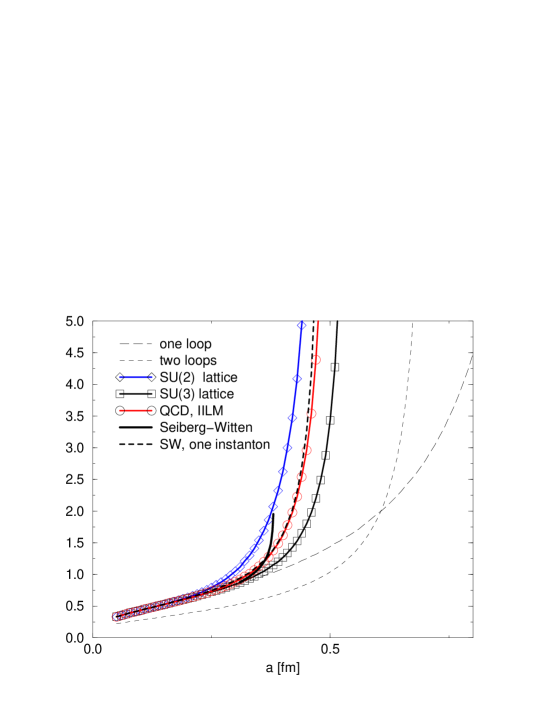
Fig. 3: The effective charge $b\,g^{2}_{eff}(\mu)/8\pi^{2}$ (b is the coefficient of the one-loop beta function) versus normalization scale $\mu$ (in units of its value at which the one-loop charge blows up). The thick solid line correspond to exact solution [24] for the N=2 SYM, the thick dashed line shows the one-instanton correction. Lines with symbols (as indicated on figure) stand for N=0 QCD-like theories, SU(2) and SU(3) pure gauge ones and QCD itself. Thin long-dashed and short-dashed lines are one and two-loop results.

Is this indeed what is happening? In order to answer such questions above I have used either lattice data or hadronic phenomenology: let me now use another tool from the theory tool-box, namely a solvable model. So we [5] are going to compare the charge in QCD to that for the N=2 supersymmetric theory, for which the famous exact effective Lagrangian was found by Seiberg and Witten [24].

$${8\pi\over g^{2}(u)}={K(\sqrt{1-k^{2}})\over K(k)}$$ (18)

where K is elliptic integral and the argument

$$k^{2}={(u-\sqrt{(}u^{2}-4\Lambda^{4}))\over(u+\sqrt{u^{2}-4\Lambda^{4}}))}$$ (19)

is a function of gauge invariant vacuum expectation of squared scalar field

$$u={1\over 2}<\phi^{2}>={a^{2}\over 2}+{\Lambda^{4}\over a^{2}}+\ldots$$ (20)

and a is just its VEV. For large $a$ there is a weak coupling expansion which includes instanton effects

$${8\pi\over g^{2}(u)}={2\over\pi}\left(\log\left({2a^{2}\over\Lambda^{2}}\right)-{3\Lambda^{4}\over a^{4}}+\ldots\right)$$ (21)

The exact coupling blows up at $u=2\Lambda^{2}$, which means that the factor between the exact strong interaction scale and the perturbative one is in this theory $\Lambda_{\infty}=2^{3/2}\Lambda$. Actually this is the ratio of the scale $\sqrt{u}$ to the scale $a$ at which the perturbatively evolved coupling (one-loop) blows up. If one were to account for the next term in the expansion of $u$, the ratio of scales is reduced to $\sqrt{2}\sqrt{2+\sqrt{2}}$. The fact that instanton effects can be important at such a high scale was anticipated in Ref. [6] and is presumably due to the significance of the pre-factor in instanton calculations.)

The behavior is shown in Fig.(3), where we have included both a curve which shows the full coupling (thick solid line), as well as a curve which illustrates only the one-instanton correction (thick dashed one). The units on both axis are chosen so that the naive one-loop running looks the same in both theories. And – surprise, surprise – the instanton-induced corrections seem to be the nearly the same as well.

I think this comparison teaches us few lessons. The main of them: if the instanton-induced corrections to the charge itself becomes large, the perturbative expansion in g have to be abandoned. I do not know what exactly one can make out of (nearly ideal) numerical matching of these two theories, QCD and N=2 SUSY gluodynamics. Note however the very rapid change of the coupling induced by instantons, although different in formulae, but so similar in the curves. It is also of interest that the full multi-instanton sum makes the rise in the coupling even more radical than with only the one-instanton correction incorporated. It is also interesting to observe that at the scale where the true coupling blows up, the perturbatively evolved coupling is still not very large. Individually, the perturbative log and instanton corrections are well defined at this region: however they cancel each other in the inverse charge. This is encouraging from the point of view of developing a consistent expansion for the instanton corrections. The rapid rise in the coupling is also encouraging in that it ensures that perturbation theory is valid almost to the point where it blows up. For a consistent picture of QCD, in which perturbation theory still appears to be applicable at the $c$-quark scale, while the theory is non-perturbative at 1 GeV, such a dramatic effect is essential.

3.2 The Chiral Scale in Spin-0 Light-Quark correlators

The physical origin of the chiral scale has been traced down to instantons-induced effects [1], for recent detailed review see [4]. The main points are: (i) the instanton-induced interaction strong and short-range, (ii) it is attractive for the pion channel, repulsive for the $\eta^{\prime}$, and (iii) (to first order) it does not affect the vector channels such as $\rho,\omega$. It explains $both$ successes and failures of the OPE sum rules, reproducing the phenomenology also for all spin-0 correlation functions [18]. So far, we have only mentioned the pion contribution, and noted that it deviates from perturbative behavior at unusually small distances.

After this prelude we return to evaluation of the short distance behavior of correlation functions in the single-instanton approximation (SIA) [18]. The main idea is that if $x-y$ is small compared to the typical instanton separation $R$, we expect that the contribution from the instanton $I=I_{*}$ closest to the points $x$ and $y$ will dominate over all others. For quark propagator in the subspace of the instanton zero modes this implies

$$S(x,y)\;=\;\sum_{IJ}\psi_{I}(x)\left(\frac{1}{T+im}\right)_{IJ}\!\!\psi^{\dagger}_{J}(y)\;\simeq\;\psi_{I_{*}}(x)\left(\frac{1}{T+im}\right)_{I_{*}I_{*}}\!\!\psi^{\dagger}_{I_{*}}(y)\;\simeq\;\frac{\psi_{I_{*}}(x)\psi^{\dagger}_{I_{*}}(y)}{m^{*}}$$ (22)

where we have approximated the diagonal matrix element by its average, $(T+im)^{-1}_{I_{*}I_{*}}\simeq N^{-1}\sum_{I}(T+im)^{-1}_{II}$, and introduced the effective mass $m^{*}$ $(m^{*})^{-1}=N^{-1}\sum\lambda^{-1}$. In the following we will use the mean field estimate $m^{*}=\pi\rho(2n/3)^{1/2}$. As a result, the propagator in the SIA looks like the zero mode propagator of a single instanton, but for a particle with an effective mass $m^{*}$.

The $\pi$ and $\eta^{\prime}$ correlators receive zero modes contributions. In the single instanton approximation, we find [18]

$$\Pi^{SIA}_{\pi,\eta^{\prime}}(x) = \pm\int d\rho\,n(\rho)\frac{6\rho^{4}}{\pi^{2}}\frac{1}{(m^{*})^{2}}\frac{\partial^{2}}{\partial(x^{2})^{2}}\left\{\frac{4\xi^{2}}{x^{4}}\left(\frac{\xi^{2}}{1-\xi^{2}}+\frac{\xi}{2}\log\frac{1+\xi}{1-\xi}\right)\right\},$$ (23)

where $\xi^{2}=x^{2}/(x^{2}+4\rho^{2})$. There is also a non-zero mode contribution to these correlation functions which is not very important.

Putting in standard instanton parameters, we find that at very short distances $x\simeq.3$ fm, this contributions to the correlator coming from the instanton zero modes are larger than the contributions included in the OPE (see Fig.4a).

For the $\eta^{\prime}$, the instanton contribution is strongly repulsive. The flip of the sign is easy to understand: the instanton corrections comes only from flavor-changing diagram $\bar{u}u\rightarrow\bar{d}d$, which has different sign in correlators of $J_{\pi 0}=(\bar{u}\gamma_{5}u-\bar{d}\gamma_{5}d)$ and $J_{\eta^{\prime}}=(\bar{u}\gamma_{5}u+\bar{d}\gamma_{5}d)$ This is because the instanton accounts for the $U(1)_{A}$ anomaly. The SIA was extended to the full pseudoscalar nonet in [18]. It was shown that simply replacing $m^{*}\to m^{*}+m_{s}$ gives a good description of $SU(3)$ flavor symmetry breaking and the $\pi,K,\eta$ correlation functions.

In the vector $\rho,\omega$ correlators the zero modes cannot contribute since the chiralities do not match. Non-vanishing contributions come from the non-zero mode propagator and from interference between the zero mode part and the leading mass correction

$$\Pi^{SIA}_{\rho}(x,y) = {\rm Tr}\left[\gamma_{\mu}S^{nz}(x,y)\gamma_{\mu}S^{nz}(y,x)\right]+2{\rm Tr}\left[\gamma_{\mu}\psi_{0}(x)\psi_{0}^{\dagger}(y)\gamma_{\mu}\Delta(y,x)\right]$$ (24)

The latter term survives even in the chiral limit, because the factor $m$ in the mass correction is cancelled by the $1/m$ from the zero mode. Also note that the result corresponds to the standard DIGA, so multi-instanton effects are not included. After averaging over the instanton coordinates, we find [20]

$$\Pi^{SIA}_{\rho}(x) = \Pi^{0}_{\rho}+\int d\rho\,n(\rho)\frac{12}{\pi^{2}}\frac{\rho^{4}}{x^{2}}\frac{\partial}{\partial(x^{2})}\left\{\frac{\xi}{x^{2}}\log\frac{1+\xi}{1-\xi}\right\}$$ (25)

Similar to the OPE, this correction is only weakly attractive at intermediate distances.

An interesting observation is the fact that it is the only singular term in the instanton contribution. In fact, the OPE of any mesonic correlator in any self dual field contains only dimension 4 operators [21]. This means that for all higher order operators either the Wilson coefficient vanishes (as it does, for example, for the triple gluon condensate $\langle g^{3}f^{abc}G^{a}_{\mu\nu}G^{b}_{\nu\rho}G^{c}_{\rho\mu}\rangle$) or the matrix elements of various operators of the same dimension cancel each other. This is a very remarkable result, because it helps to explain the success of QCD sum rules based on the OPE in a number of channels. In the instanton model, the gluon fields are very inhomogeneous, so one would expect that the OPE fails for $x\ll\rho$. The Dubovikov-Smilga result shows how many observables can be absolutely blind to very strong gauge fields, as long as they are locally self dual.

3.3 Instantons and the duality scale for $J^{PC}=O^{\pm}$ glueballs

Let me first explain qualitatively why in this case the scale should be larger than in the light quark channels. The reason is the gluonic field strength inside instantons is very large.

The magnitude of the color fields inside the instanton is $O(1/g)$, and in the correlation functions in question (such as $<G^{2}(x)G^{2}(y)>$) it enters in the 4-th power. Therefore, the instanton correction is proportional to the action of the instanton squared, $(8\pi^{2}/g^{2})^{2}\sim 100$ where for estimate we have used the action to be of the order of 10. The corresponding correction with light quarks have zero modes instead of gluonic field strength, and its integral over space is not the action but just one, from the normalization of fermionic mode. So we speak about enhancement of roughly 2 orders of magnitude.

For one-instanton calculation we can start from expansion of the gluon operators around the classical fields. In the lowest order one should simply insert the classical field of an instanton into the operators, it leads to [18]

$$\Pi_{S,P}^{SIA}(x) = \int d\rho\,n(\rho)\frac{8192\pi^{2}}{g^{4}\rho^{4}}\frac{\partial^{3}}{\partial(x^{2})^{3}}\left\{\frac{\xi^{6}}{x^{6}}\left(\frac{10-6\xi^{2}}{(1-\xi^{2})^{2}}+\frac{3}{\xi}\log\frac{1+\xi}{1-\xi}\right)\right\}$$ (26)

where $\xi$ is defined as in (23). There is no classical contribution in the tensor channel, since the stress tensor in the self-dual field of an instanton is zero. Note that the perturbative contribution in the scalar and pseudoscalar channels have opposite sign, while the classical contribution has the same sign. To first order in the instanton density, we therefore find all three scenarios : attraction in the scalar channel, repulsion in the pseudoscalar and no effect in the tensor channel.

The single-instanton prediction can be compared with the OPE, and it is much larger indeed. Furthermore, if one uses the standard $\rho,n$ of the instanton vacuum, it matches it the scale inferred from low energy theorem very well.

Numerical calculations of glueball correlators in different instanton ensembles were performed in [22]. At short distances, the results are consistent with the single instanton approximation. At larger distances, the scalar correlator is modified due to the presence of the gluon condensate. This means that (like the $\sigma$ meson), the correlator has to be subtracted and the determination of the mass is difficult. In the pure gauge theory we find $m_{0^{++}}=1.5$ GeV. While the mass is consistent with QCD sum rule predictions, the coupling is much larger than expected from calculations that do not enforce the low energy theorem.

In [22] we also measured glueball wave functions. The most important result is that the scalar glueball is indeed small, $r_{0^{++}}=.2$ fm and determined by the size of an instanton, while the tensor is much bigger, sensitive to interactions at the size determined by the average distance between instantons 1 fm.

In the pseudoscalar channel the correlator is very repulsive and there is no clear indication of a glueball state. In the full theory (with quarks) the correlator is modified due to topological charge screening. The non-perturbative correction changes sign and a light (on the scale of the glueballs) state, the $\eta^{\prime}$ appears. Non-perturbative corrections in the tensor channel are tiny. Isolated instantons and anti-instantons have a vanishing energy momentum tensor, so the result is entirely due to interactions.

4 Confinement effects at small distances

4.1 Instanton Suppression

The central idea of this Section is that $O(\rho^{2})$ suppression of instantons can be due to a “dual superconductivity” [23], a scenario in which some composite objects condense, forming the non-zero vacuum expectation value (VEV) of the magnetically charged scalar field $\phi$. My first (naive) argument was that in such theory, unlike the QCD itself, at least there is the dimension-2 operator $|\phi|^{2}$.

The composites may be magnetic monopoles [23, 24], or P-vortices, or something else: anyway one is lead to an incarnation of the old Landau-Ginzburg effective theory, Abelian Higgs Model (AHM), describing interaction of a “dual photon” and “dual Higgs” fields. AHM was applied to the description of the QCD strings, as Abrikosov-Nielsson-Olesen vortices [25].

Before we go into details, let us point out a striking similarity between these two problems. A vortex is the 2d topologically non-trivial configuration, in which $\phi$ vanishes at the center, the Dirac string where the dual potential must be singular. An instanton problem is in a way the previous one squared. The 4d picture of the fields is like two string cross sections in two orthogonal 2d planes. Higgs field $\phi$ again vanishes at the center, because in the singular gauge (the only one good for multi-instanton configurations) the gauge field is $A_{\mu}(x)^{2}\sim 1/x^{2}$ at the origin, acting as a centrifugal barrier. Since “melting” of the dual superconductor at the center is not a small modification, one generally cannot expect the OPE-type calculations to hold. In both problems one has first to solve for the field and then calculate the energy or action. Fortunately, for instantons in a Higgsed vacuum it was already done by ’t Hooft [14]: for fundamentally charged Higgs the answer is

$$\Delta S=4\pi^{2}\rho^{2}|<\Phi>|^{2}$$ (27)

Note that it leads to the $O(\rho^{2})$ suppression law we need to explain Fig.[1](b), and that $\Delta S$ should not necessarily be small. We return to speculations on the exact nature of the Higgs and the dual photon fields of the Landau-Ginzburg model (needed to evaluate the strength of the effect) below.

Encouraged by this, we return to instantons and try to apply the same reasoning. Since both the ’t Hooft correction (27) and the string tension (30) scales as the Higgs VEV squared, we expect qualitatively that

$${dN\over d\rho}={dN\over d\rho}|_{pert}exp{(-C\sigma\rho^{2})}$$ (28)

where C is some numerical constant. In order to find C one has to identify the scalar and the dual photon fields of the AHM, and explain how they are coupled to the colored gauge field of the instanton. In the AHM treatment of the QCD string [28] the magnetic field of the dual photon is identified directly with the color-electric gauge field inside the string. It does not create problems because this electric field can be considered Abelian.

Applying the same ideas for instantons, let us first note that their $self-duality$ helps: because electric and magnetic fields are identical, the “magnetic” potential $C_{\mu}$ and the original one $A_{\mu}$ are also the same. However both are intrinsically non-Abelian, so only a particular component (or a combination of those) can be identified with the Abelian “dual photon” of the effective theory. In other words, an Abelian projection is inevitable, and there is no unique or preferred way to do it. Lacking better ideas, we simply do what lattice people do: just select one of possible projections and see what happens. Clearly, selecting Higgs field interacting with a particular component of the gauge potential means breaking the gauge group (which the vacuum of the Standard model does and that of QCD does not). But we proceed anyway, simply re-scaling the dual fields in a way that their Lagrangian (1) matches the ’t Hooft one. If we do so, it leads to identification $<\Phi>^{2}=(2/3)\phi_{0}^{2}$, or the constant C in (28) to be $C=2\pi$. Putting it all together, we can now compare this result to the exponential suppression. The corresponding curves are shown in Fig.1, and it works very well.

Brief summary. The “dual superconductivity” leading to confinement in the QCD vacuum seems to be surprisingly robust. Instanton suppression and/or string tension considered before both fix the AHS Higgs VEV rather accurately. The string size and small-r potential provide hints that the Higgs and dual photon masses are large, in the 1-1.5 GeV range. Their exact nature remains unclear.

Outlook: one may test our suggestions by comparing instanton suppression in theories with variable number of colors and/or flavors. Unfortunately available data for the SU(2) color group or SU(3) with dynamical fermions are not yet good enough to do so.

Another challenging set of questions is related with instanton suppression at non-zero temperatures T and/or densities. At high T or density, in the quark-gluon plasma phase, the answer is clear: the instanton electric fields are again suppressed, but now by the usual Debye screening[34]. It leads to a factor $exp(-a(T,\mu)\rho^{2})$ similar to the one discussed above, where the coefficient $a(T,\mu=0)$ was calculated in [35] and then generalized to the $\mu\neq 0$ in [1]. Note that confinement is not completely gone: it remains for spatial Wilson loops. The most interesting point is what happens close to the deconfinement transition. Since 2 and 3 color gouge theories have it of the second and the first kind, respectively, a detailed study of the instanton suppression at $T\approx T_{c}$ is of great interest.

4.2 Long and Short Strings

Now we briefly review applications of the dual superconductivity idea to the QCD string, or the ANO vortex line, done in a series of papers [29]. Among clear successes of this approach is: (i) prediction of weak string-string interaction, putting it around the boundary of type I and II superconductivity; (ii) prediction of a whole set of potentials other than central. Both agree well with available lattice data, for a review see [17].

The effective Lagrangian used in [28] is

$$L={4\over 3}[{1\over 4}(\partial_{\mu}C_{\nu}-\partial_{\nu}C_{\mu})^{2}+$$ (29)

$${1\over 2}|(\partial_{\mu}-ig_{m}C_{\mu})\phi|^{2}+{\lambda\over 4}(|\phi|^{2}-|\phi_{0}|^{2})^{2}]$$

where we have omitted interaction with quarks at the ends. $C_{\mu}$ is dual color potential coupled to Higgs with magnetic coupling $g_{m}=2\pi/g$. Assuming that we are exactly at the boundary of the type I and II superconductivity, the masses of the Higgs and the “dual photon” are equal $M_{\phi}=M_{C}=g_{m}\phi_{0}$. The (classical) string tension is directly related to Higgs VEV

$$\sigma={4\pi\over 3}|\phi_{0}|^{2}$$ (30)

In effective dual model [28] the string width is related to masses of dual photon and Higgs, being the large non-perturbative scale of the 3-ed kind we are speaking about. The data mentioned put it in the “glueball mass range”, around 1.3 GeV according to Fig.2b (It is difficult for me to access the error involved.)

5 QCD Vacuum as the Instanton Liquid

5.1 The qualitative picture

It was already mentioned that, as pointed out in [1], the typical instanton size is significantly smaller than their separation $R=n^{-1/4}\approx 1fm$, or

$$\rho_{\rm max} \sim 1/3\,{\rm fm}.$$ (31)

If so, the following qualitative picture of the QCD vacuum emerges

1. Since the instanton size is significantly smaller than the typical separation $R$ between instantons, $\rho/R\sim 1/3$, the vacuum is fairly dilute. The fraction of spacetime occupied by strong fields is only a few per cent.

2. The fields inside the instanton are very strong $G_{\mu\nu}\gg\Lambda_{QCD}^{2}$. This means that the semi-classical approximation is valid, and the typical action is large

   $$S_{0}=8\pi^{2}/g^{2}(\rho)\sim 10-15\gg 1.$$ (32)

   Higher order corrections are proportional to $1/S_{0}$ and presumably small.

3. Instantons retain their individuality and are not destroyed by interactions. From the dipole formula, one can estimate

   $$|\delta S_{int}|\sim(2-3)\ll S_{0}.$$ (33)

4. Nevertheless, interactions are important for the structure of the instanton ensemble, since

   $$\exp|\delta S_{int}|\sim 20\gg 1.$$ (34)

   This implies that interactions have a significant effect on correlations among instantons, the instanton ensemble in QCD is not a dilute gas, but an interacting liquid.

The aspects of the QCD vacuum for which the instantons are most important are those related with light fermions. Their importance in the context of chiral symmetry breaking is related to the fact that the Dirac operator has a chiral zero mode in the field of an instantons. These zero modes are localized quark states around instantons, like atomic states of electrons around nuclei. At finite density of the instantons those states can become collective, like atomic states in metals. The resulting de-localized state corresponds to the wave function of the quark condensate.

5.2 How to calculate?

In this lectures there is no place for technical details, which may be found in the original papers. Rather we try to explain the logical structure and possible alternatives of the theory. For that reason, discussion of possible methods to calculate something with instantons is put into the introduction, with only results of the calculation reported below.

In the QCD partition function there are two types of fields, gluons and quarks, and so the first question one addresses is which integral to take first.

(i) One way is to eliminate $gluonic$ degrees of freedom first. Physical motivation for that may be that gluonic states are heavy and an effective fermionic theory should be better suited to derive an effective low-energy theory. In the instanton framework, this approach was started by ’t Hooft who discovered that instantons lead to new effective interactions between light quarks. We will present the explicit form of such four-fermion interaction for two-flavor QCD below.

It is a well-trotted path and one can follow it along the development for a similar four-fermion theory, the NJL model. One can do simple mean field or random field approximation (RPA) diagrams, and find the mean condensate and properties of the mesons. Unfortunately, it is difficult to do more. For example, baryons are states with three quarks, and using quasi-local four-fermion Lagrangians for the three body problem is technically a very difficult (although solvable) quantum mechanical problem. There were no attempts to sum more complicated diagrams.

(ii) The opposite strategy can be to do $fermion$ integral first. It is a simple step, because they only enter quadratically, leading to a fermionic determinant. This is the way lattice people proceed. In the instanton approximation, it leads to the Interacting Instanton Liquid Model, defined by the following partition function:

$$Z=\sum_{N_{+},\,N_{-}}{1\over N_{+}!N_{-}!}\int\prod_{i}^{N_{+}+N_{-}}[d\Omega_{i}\;d(\rho_{i})]\exp(-S_{\rm int})\prod_{f}^{N_{f}}\det(\hat{D}+m_{f})\,,$$ (35)

describing a system of pseudo-particles interacting via the bosonic action and the fermionic determinant. Here $d\Omega_{i}=dU_{i}\,d^{4}z_{i}\,d\rho_{i}$ is the measure in color orientation, position and size, associated with single instantons and $d(\rho)$ is the single instanton density $d(\rho)=dn_{I,\bar{I}}/d\rho dz$.

The gauge interaction between instantons is approximated by a sum of pure two-body interaction $S_{\rm int}=\frac{1}{2}\sum_{I\neq J}S_{\rm int}(\Omega_{IJ})$. Genuine three body effects in the instanton interaction are not important as long as the ensemble is reasonably dilute. Implementation of this part of the interaction (quenched simulation) is quite analogous to usual statistical ensembles made of atoms.

As already mentioned, quark exchanges between instantons are included in the fermionic determinant. Finding a diagonal set of fermionic eigenstat es of the Dirac operator is similar to what people are doing, e.g., in quantum chemistry when electron states for molecules are calculated. The difficulty of our problem is however much higher, because this set of fermionic states should be determined for $all$ configurations which appear during the Monte-Carlo process.

If the set of fermionic states is however limited to the subspace of instanton zero modes, the problem becomes tractable numerically. Typical calculations in the IILM involved up to N$\sim 100$ instantons (+anti-instantons): it means that the determinants of $N\times N$ matrices are involved. Such determinants can be evaluated by the ordinary workstation (and even PC these days) so quickly, that straightforward Monte Carlo simulation of IILM is possible in a matter of minutes. On the other hand, expanding the determinant in a sum of products of matrix elements, one can easily identify the sum of all closed loop diagrams up to order $N$ in the ’t Hooft interaction. Thus, in this way we take care of (practically) all orders!

5.3 Correlation functions

Fig. 4: Pion correlation function in various approximations and instanton ensembles. In the top figure we show the phenomenological expectation (solid), the OPE (dashed), the single instanton (dash-dotted) and mean field approximations (dashed) as well as data in the random instanton ensemble. In the bottom figure we compare different instanton ensembles, random (open squares), quenched (circles) and interacting (streamline: solid squares, ratio ansatz solid triangles).

There is no place here to explain the details of how we performed calculations in the Interacting Instanton Liquid Model (IILM): they are done by Monte Carlo, in a way not so different from standard methods used in other statmech models. Different versions of the model (mentioned in figures below as IILM(rat) etc) differ by a particular ansatz for gauge field used, from which the interaction is calculated. Note also, that these figures mostly contain also a curve marked “phen”: this is how the correlator actually look like, according to phenomenology.

We simply jump to show a sample of results. Correlation functions in the different instanton ensembles were calculated in several papers (see original refs in [4]). Some of them (like vector and axial-vector ones) turned out to be easy: nearly any variant of the instanton model can reproduce well the (experimentally known!) correlators. Some of them are sensitive to details of the model very much: two such cases are shown in Figs. 4-5. The pion correlation functions in the different ensembles are qualitatively very similar. The differences are mostly due to different values of the quark condensate (and the physical quark mass) in the different ensembles. Using the Gell-Mann, Oaks, Renner relation, one can extrapolate the pion mass to the physical value of the quark masses. The results are consistent with the experimental value in the streamline ensemble (both quenched and unquenched), but clearly too small in the ratio ansatz ensemble. This is a reflection of the fact that the ratio ansatz ensemble is not sufficiently dilute.

Fig. 5: Eta prime meson correlation functions. The various curves and data sets are labeled as in Fig. 4.

Fig. 6: Rho meson correlation functions. The various curves and data sets are labeled as in Fig. 4. The dashed squares show the non-interacting part of the rho meson correlator in the interacting ensemble.

In Fig. 6 we also show the results in the $\rho$ channel. The $\rho$ meson correlator is not affected by instanton zero modes to first order in the instanton density. The results in the different ensembles are fairly similar to each other and all fall somewhat short of the phenomenological result at intermediate distances $x\simeq 1$ fm. We have determine the $\rho$ meson mass and coupling constant from a fit. The $\rho$ meson mass is somewhat too heavy in the random and quenched ensembles, but in very good agreement with the experimental value $m_{\rho}=770$ MeV in the interacting ensemble.

Since there are no interactions in the $\rho$ meson channel in the RPA, it is important to study whether the instanton model provides any binding at all. In the instanton model, there is no confinement, and $m_{\rho}$ is close to the two (constituent) quark threshold. In QCD, the $\rho$ meson is also not a true bound state, but a resonance in the 2$\pi$ continuum. In order to determine whether the continuum contribution in the instanton model is predominantly $2\pi$ or 2 quark would require the determination of the corresponding three point functions (which has not been done yet). Instead, we will compare the full correlation function with the non-interacting one, where we use the average (constituent quark) propagator determined in the same ensemble (Fig. 6). As explained above, this comparison provides a measure of the strength of interaction. We observe that there is an attractive interaction generated in the interacting liquid. The interaction is due to correlated instanton-anti-instanton pairs. This is consistent with the fact that the interaction is considerably smaller in the random ensemble. In the random model, the strength of the interaction grows as the ensemble becomes more dense. However, the interaction in the full ensemble is significantly larger than in the random model at the same diluteness. Therefore, most of the interaction comes from dynamically generated pairs.

The situation is drastically different in the $\eta^{\prime}$ channel. Among the $\sim 40$ correlation functions calculated in the random ensemble, only the $\eta^{\prime}$ and the isovector-scalar $\delta$ were found to be completely unacceptable: The correlation function decreases very rapidly and becomes $negative$ at $x\sim 0.4$ fm. This behavior is incompatible even with a normal spectral representation. The interaction in the random ensemble is too repulsive, and the model “over-explains” the $U(1)_{A}$ anomaly.

The results in the unquenched ensembles (closed and open points) significantly improve the situation. This is related to dynamical correlations between instantons and anti-instantons (topological charge screening). The single instanton contribution is repulsive, but the contribution from pairs is attractive. Only if correlations among instantons and anti-instantons are sufficiently strong, the correlators are prevented from becoming negative. Quantitatively, the $\delta$ and $\eta_{\rm ns}$ masses in the streamline ensemble are still too heavy as compared to their experimental values. In the ratio ansatz, on the other hand, the correlation functions even show an enhancement at distances on the order of 1 fm, and the fitted masses are too light. This shows that the $\eta^{\prime}$ channel is very sensitive to the strength of correlations among instantons.

In summary, pion properties are mostly sensitive to global properties of the instanton ensemble, in particular its diluteness. Good phenomenology demands $\bar{\rho}^{4}n\simeq 0.03$, as originally suggested in[1]. The properties of the $\rho$ meson are essentially independent of the diluteness, but show sensitivity to $\bar{I}I$ correlations. These correlations become crucial in the $\eta^{\prime}$ channel.

5.4 Baryonic correlation functions

Existence of a strongly attractive interaction in the pseudoscalar quark-antiquark (pion) channel also implies an attractive interaction in the scalar quark-quark (diquark) channel. This interaction is phenomenologically very desirable, because it immediately explains why the nucleon and lambda are light, while the delta and sigma are heavy.

The proton currents (with no derivatives and the minimum number of quark fields) with positive parity and spin $1/2$ are given by[26]. It is useful to rewrite these currents in terms of scalar and pseudoscalar diquarks

$$\eta_{1,2} = (2,4)\left\{\epsilon_{abc}(u^{a}Cd^{b})\gamma_{5}u^{c}\mp\epsilon_{abc}(u^{a}C\gamma_{5}d^{b})u^{c}\right\}.$$ (36)

Nucleon correlation functions are defined by $\Pi^{N}_{\alpha\beta}(x)=\langle\eta_{\alpha}(0)\bar{\eta}_{\beta}(x)\rangle$, where $\alpha,\beta$ are the Dirac indices of the nucleon currents. In total, there are six different nucleon correlators: the diagonal $\eta_{1}\bar{\eta}_{1},\,\eta_{2}\bar{\eta}_{2}$ and off-diagonal $\eta_{1}\bar{\eta}_{2}$ correlators, each contracted with either the identity or $\gamma\cdot x$. Let us focus on the first two of these correlation functions (for more detail, see[4] and references therein).

Fig. 7: Nucleon and delta correlation functions $\Pi_{2}^{N}$ and $\Pi_{2}^{\Delta}$. Curves labeled as in Figs. 4-6.

The correlation function $\Pi_{2}^{N}$ in the interacting ensemble is shown in Fig. 7. There is a significant enhancement over the perturbative contribution which is nicely described in terms of the nucleon contribution. Numerically, we find $m_{N}=1.019$ GeV. In the random ensemble, we have measured the nucleon mass at smaller quark masses and found $m_{N}=0.96\pm 0.03$ GeV. The nucleon mass is fairly insensitive to the instanton ensemble. However, the strength of the correlation function depends on the instanton ensemble. This is reflected by the value of the nucleon coupling constant, which is smaller in the IILM. In[33] we studied all six nucleon correlation functions. We showed that all correlation functions can be described with the same nucleon mass and coupling constants.

The fitted value of the threshold is $E_{0}\simeq 1.8$ GeV, indicating that there is little strength in the “three quark continuum” (dual to higher resonances in the nucleon channel). The fact that the nucleon in IILM is actually bound can also be demonstrated by comparing the full nucleon correlation function with that of three non-interacting quarks (the cube of the average propagator. The full correlator is significantly larger than the non-interacting one.

Significant part of this interaction was traced down to strongly attractive scalar diquarks. The nucleon (at least in IILM) is a strongly bound diquark, plus a loosely bound the third quark.

The properties of this diquark picture of the nucleon continue to be disputed by phenomenologists. We would return to diquarks in the next section, where they would become Cooper pairs of Color Superconductors.

In the case of the $\Delta$ resonance, there exists only one independent current, given (for the $\Delta^{++}$) by

$$\eta^{\Delta}_{\mu}=\epsilon_{abc}(u^{a}C\gamma_{\mu}u^{b})u^{c}.$$ (37)

However, the spin structure of the correlator $\Pi^{\Delta}_{\mu\nu;\alpha\beta}(x)=\langle\eta^{\Delta}_{\mu\alpha}(0)\bar{\eta}^{\Delta}_{\nu\beta}(x)\rangle$ is much richer. In general, there are ten independent tensor structures, but the Rarita-Schwinger constraint $\gamma^{\mu}\eta_{\mu}^{\Delta}=0$ reduces this number to four.

The mass of the delta resonance is too large in the random model, but closer to experiment in the unquenched ensemble. Note that similar to the nucleon, part of this discrepancy is due to the value of the current mass. Nevertheless, the delta-nucleon mass splitting in the unquenched ensemble is $m_{\Delta}-m_{N}=409$ MeV, larger but comparable to the experimental value 297 MeV. It mostly comes from the absence of attractive scalar diquarks in this channel.

6 The Phases of QCD

Turning to finite temperature/density QCD now, let me start with emphasizing its main goals. Those are not to use once again a semi-classical or perturbative calculations, similar to what have been done before in vacuum. What we are looking for here are new phases of QCD (and related theories), namely new self-consistent solutions which differs qualitatively from what we have in the QCD vacuum.

One such phase occurs at high enough temperature $T>T_{c}$: it is known as Quark Gluon Plasma (QGP). It is a phase understandable in terms of basic quark and gluon-like excitations [34], without confinement and with unbroken chiral symmetry in the massless limit. One of the main goals of heavy ion program, especially at new Brookhaven dedicated facility RHIC, is to study transitions to this phase.

Another one, which gets much attention recently, is the direction of finite density. Very robust Color Superconductivity was found to be the case here. Let me also mention one more frontier $not$ to be discussed below, which has not yet attracted sufficient attention: namely transition (or many transitions?) as the number of light flavors $N_{f}$ grows. The minimal scenario includes transition from the usual hadronic phase to one more unusual QCD phase, the $conformal$ one, in which there are no particle-like excitations and correlators are power-like in the infrared. Even the position of the critical point is unknown.

That the main driving force of these studies is the intellectual challenge it provides. In order to prove to you that the problems related with mechanism of confinement and chiral symmetry breaking are not simple, it is enough to remind that a lot of people who moved these days into quantum gravity/string theory did so partly because of frustration with the non-perturbative QCD. However I still think that, with the help of all experimental data, real and numerical, we have at hand for QCD we still have much better chances here.

6.1 The Phase diagram

The QCD phase diagram version circa 1999 [44] is shown in Fig 8(a), at the baryonic chemical potential $\mu$ (normalized per quark, not per baryon) - the temperature T plane. Some part of it is old: it is hadronic phase at small values of both parameters, and QGP phase at large T,$\mu$.

The phase transition line separating them most probably does not really start at $T=T_{c},\mu=0$ but at a “endpoint” E, a remnant of the so called QCD tricritical point which QCD has in the chiral (all quarks are massless) limit. Although we do not know where it is, we hope we know how to find it, see [43]. The proposed ideas rotate around the fact that the order parameter, the VEV of the sigma meson, is at this point truly massless, and creates a kind of a “critical opalesence”. Similar phenomena were predicted and then indeed observed at the endpoint of another line (called M from multi-fragmentation), separating liquid nuclear matter from nuclear gas phase.

The large-density (and low-T) region looks rather different from what was shown at conferences just few months ago: there appear two new Color Super-conducting phases there. Unfortunately heavy ion collisions do not cross this part of the phase diagrams, and so it belongs to a neutron star physics.

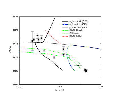
Fig. 8: (a) Schematic phase diagram of QCD, in temperature T- baryon chemical potential $\mu$ plane. E and M show critical endpoints of first order transitions: M (from multi-fragmentation) is that for liquid-gas transition in nuclear matter. The color superconducting phases, CSC2 and CSC3 are explained in the text. (b) The part of the phase diagram which has been experimentally accessible by heavy ion collisions. Closed (open) points correspond to chemical (thermal) freeze-out. The zigzag is the adiabatic paths correspond to entropy per baryon ratio indicated. Lines of thermal freeze-out for central sulfur-sulfur and PbPb collisions, as well as the initial line for PbPb are also indicated.

The 2-flavor-like color superconductor CSC2 phase was known before [37], but realization that it should be induced by instantons [40, 41] has increased the gaps (and $T_{c}$) from a few MeV scale to $\sim$100 MeV (50 MeV). In the hindsight is should hardly be surprising, since the $same$ interaction in $\bar{q}q$ channel is responsible for chiral symmetry breaking, producing the gap (the constituent quark mass) as large as 350-400 MeV. Furthermore, in the two-color QCD, there is the so called Pauli-Gursey symmetry which relates these two condensates. So at high density the chiral condensate $<\bar{q}q>$ simply rotates into superconductor one $<qq>$, while the gap remains the same.

The symmetries of the CSC2 phase are similar to the electroweak part of the Standard Model, with the condensed scalar isoscalar $ud$ diquark operating as Higgs. The colored condensate breaks the color group, making 5 out of 8 gluons massive. The 3-flavor-like phase, CSC3, is brand new: it was proposed in [42] based on one gluon exchange interaction, but in fact it is favored by instantons as well [44]. Its unusual features include color-flavor locking and coexistence of both types of condensates, $<qq>$ and $<\bar{q}q>$. It combines features of the Higgs phase (8 massive gluons) and of the usual hadronic phase (8 massless “pions”).

Above I mention approach to high density starting from the vacuum. One can also work out in the opposite direction, starting from very large densities and going down. As it was noticed in ref. [47], electric part of one-gluon exchange is screened, and therefore the Cooper pairs appears due to magnetic forces. It is interesting by itself, as a rare example: one has to take care of time delay effects of the interaction. The result is the indefinitely growing gaps at large $\mu>10GeV$, as $\Delta\sim\mu exp(-{3\pi^{2}\over\sqrt{2}g(\mu)})$.

6.2 Finite T transition and Large Number of Flavors

There is no place here to discuss this subject in details: there are rather extensive lattice data now, and so we actually know quite a lot about these transition.

Let me only emphasize what it is look like from the perspective of the instanton-based theory. If the near-random set of instantons leads to chiral symmetry breaking and quasi-zero modes at low T, we should be able to explain in the same terms how the high-T phase look like. The simplest solution would be just disappearance of instantons at $T>T_{c}$, and at some early time people thought this is what actually happens. However, it should not be like this because the Debye screening which is killing them only appears at $T=T_{c}$. Lattice data works have also found no depletion of the instanton density up to $T=T_{c}$.

On the other hand, the absence of the condensate and quasi-zero modes can only mean that the “liquid” is now broken into finite pieces. The simplest of them are pairs, or the instanton-anti-instanton molecules. This is precisely what instanton simulations have found [4]. Whether it is or is not so on the lattice is not yet clear. Some nice molecules were located, but the evidences for the molecular mechanism are still far from being completely convincing. No alternative have been so far proposed, however.

The results of simulations with $N_{f}=2,3,5$ flavors with equal masses can be summarized as follows. For $N_{f}=2$ there is second order phase transition which turns into a line of first order transitions in the $m-T$ plane for $N_{f}>2$. If the system is in the chirally restored phase ($T>T_{c}$) at $m=0$, we find a discontinuity in the chiral order parameter if the mass is increased beyond some critical value. Qualitatively, the reason for this behavior is clear. While increasing the temperature increases the role of correlations caused by fermion determinant, increasing the quark mass has the opposite effect. We also observe that increasing the number of flavors lowers the transition temperature. Again, increasing the number of flavors means that the determinant is raised to a higher power, so fermion induced correlations become stronger. For $N_{f}=5$ we find that the transition temperature drops to zero and the instanton liquid has a chirally symmetric ground state, provided the dynamical quark mass is less than some critical value. Studying the instanton ensemble in more detail shows that in this case, all instantons are bound into molecules.

Unfortunately, little is known about QCD with different numbers of flavors from lattice simulations. There are data by the Columbia group for $N_{f}=4$. The most important result is that chiral symmetry breaking effects were found to be drastically smaller as compared to $N_{f}=0,2$. In particular, the mass splittings between chiral partners such as $\pi-\sigma,\,\rho-a_{1},\,N(\frac{1}{2}^{+})-N(\frac{1}{2}^{-})$, extrapolated to $m=0$ were found to be 4-5 times smaller. This agrees well with what was found in the interacting instanton model: more work in this direction is certainly needed.

6.3 Color superconductivity

My interest was initiated by finding [33] that in the instanton liquid model even without $any$ quark matter, the ud scalar diquarks are very deeply bound, by amount comparable to the constituent quark mass. So, phenomenological manifestations [39] of such diquarks have in fact deep dynamical roots: they follow from the same basic dynamics as the “superconductivity” of the QCD vacuum, the chiral ($\chi$-)symmetry breaking. These spin-isospin-zero diquarks are related to pions, and should be quite robust element of nucleon (octet baryons) structure .

Another argument for deeply bound diquarks comes from bi-color ($N_{c}=2$) theory: in it the scalar diquark is degenerate with pions. By continuity from $N_{c}=2$ to $3$, a trace of it should exist in real QCD.

Explicit calculations with instanton-induced forces for $N_{f}=2,N_{c}=3$ QCD have been made in two simultaneous papers [40, 41]. Indeed, a very robust Cooper pairs and gaps $\Delta\sim$ 100 MeV were found. From then on, the field is booming.

Instantons create the following amusing triality: there are three attractive channels which compete: (i) the instanton-induced attraction in $\bar{q}q$ channel leading to $\chi$-symmetry breaking. (ii) the instanton-induced attraction in $qq$ which leads to color superconductivity. (iii) the light-quark-induced attraction of $\bar{I}I$, which leads to pairing of instantons into “molecules” and a Quark-Gluon Plasma (QGP) phase without $any$ condensates.

How the calculations are actually made?. Analytically, mostly in the mean field approximation, similar to the original BCS theory in Gorkov formulation. Total thermodynamical potential consists of “kinetic energy” of the quark Fermi gas, including mass operators of two types (shown in figure below). The “potential energy” in such approximation is the interaction Lagrangian convoluted with all possible condensates. For example, instanton-induced one with $N_{f}=3$ leads to two types of diagrams shown in Fig.4, with (a) $<\bar{q}q>^{3}$ and (b) $<qq>^{2}<\bar{q}q>$. Then one minimizes the potential over all condensates and get gap equations: algebra may be involved because masses/condensates are color-flavor matrices.

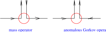
Fig. 9: (a) Two mass operators; (b) and example of two contribution to the potential energy for 3 flavor theory, including cube of the $<\bar{q}q>$ and $|<qq>|^{2}<\bar{q}q>$.

Bi-color QCD: a very special theory One reason it is special is well known to lattice community: its fermionic determinant is $real$ even for non-zero $\mu$, which makes simulations possible.

However the major interest to this theory is related the so called Pauli-Gursey symmetry. We have argued above that pions and diquarks appear at the same one-instanton level, and are so to say brothers. In bi-color QCD they becomes identical twins: due to additional symmetry mentioned the diquarks are degenerate with mesons.

In particular, the $\chi$-symmetry breaking is done like this $SU(2N_{f})\rightarrow Sp(2N_{f})$, and for $N_{f}=2$ the coset $K=SU(4)/Sp(4)=SO(6)/SO(5)=S^{5}$. Those 5 massless modes are pions plus scalar diquark S and its anti-particle $\bar{S}$.

Vector diquarks are degenerates with vector mesons, etc. Therefore, the scalar-vector splitting is in this case about twice the constituent quark mass, or about 800 MeV. It should be compared to binding in the “real” $N_{c}=3$ QCD of only 200-300 MeV, and to zero binding in the large-$N_{c}$ limit.

The corresponding sigma model describing this $\chi$-symmetry breaking was worked out in [40]: for further development see [50]. As argued in [40], in this theory the critical value of transition to Color Superconductivity is simply $\mu=m_{\pi}/2$, or zero in the chiral limit. The diquark condensate is just rotated $<\bar{q}q>$ one, and the gap is the constituent quark mass. Recent lattice works [49] and instanton liquid simulation [51] display it in great details, building confidence for other cases.

Two flavor Three color QCD: the CSC2 phase The first studies of instanton-induced CSC were made for this theory: [40, 41, 46]. The gap around 100 MeV was found, and the main point is a competition between the usual $\chi$-symmetry breaking (pairing in the $\bar{q}q$ channel) with CSC (pairing in the $qq$ channel). In the corresponding high density phase we called CSC2 the chiral symmetry is simply restored.

In all these works one more possible phase (intermediate between vacuum and CSC2), Fermi gas of constituent quarks, with both $M,\Delta\neq 0$ - was unstable. However in last more refined calculation [44] it obtains a small window. Its features are amusingly close to those of nuclear matter: but it isn’t, of course: to get nucleons one should go outside the mean field. First attempted to do so in [44] was for another cluster - the $\bar{I}I$ molecules. At T=0 it is however only 10% correction to previous results, but is dominant as T grows.

Three color Three flavor QCD produces a new phenomenon called color-flavor locking [42]. It means that the diquark condensate has the following structure $\langle q_{i}^{a}Cq_{j}^{b}\rangle=\bar{\Delta}_{1}\delta_{ia}\delta_{bj}+\bar{\Delta}_{2}\delta_{ib}\delta_{ja}$, where ij are color and ab flavor indices. It is very symmetric, reducing $SU(3)_{c}SU(3)_{f}\rightarrow SU(3)_{diagonal}$. We call it the CSC3 phase: it still breaks chiral symmetry.

It was verified to be the lowest in [42] for the one gluon exchange interaction (adequate for high density): in this case only ¡qq¿ condensate exists. About the same phase appears for the instanton-induced Lagrangian (adequate for intermediate density) [44]: but now the $<\bar{q}q>$ condensates are non-zero as well. The color-flavor locking is probably always the case for that theory.

Gaps $\delta_{i}$ and masses $\sigma_{i}$ (proportional to $<\bar{q}q>$), following from instanton-based calculation [44], are shown as a function of $\mu$ in the following figure

Physics issues under discussion for CSC3 include hadron-quark continuity. As pointed out in [53], the CSC3 phase not only has the same symmetries as hadronic matter (e.g. broken $\chi$-symmetry), but also very similar excitations. 8 gluons become 8 massive vector mesons, 3*3 quarks become 8+1 “baryons”. The 8 massless pions remain massless. Furthermore, photon and gluons are combined into a massless $\gamma_{inside}$. Calculation of masses and coupling constants of all of them is now in progress. Can these phases be $distiquished$, and should there be $any$ phase transition in the $N_{f}=3$ theory, separating it from nuclear matter? There is no need for it, at least from symmetry point of view.

The realistic QCD(Two light plus strange flavor) was studied in several papers [44, 52]. Just kinematically it is easy to see that us,ds Cooper pairs with zero momentum is difficult to make: for $\mu_{u,d}=\mu_{s}$ the momenta $p^{F}_{u,d}\neq p^{F}_{s}$. Instantons generate also a dynamical operator $m_{s}(\bar{u}\bar{d})(ud)$. Resulting behavior is as shown in our first figure.

Asymptotically large densities At $\mu>>1GeV$ the instantons are Debye-screened [1], as well as the electric (Coulomb) gluons. So magnetic gluons overtake electric ones [47]. $Magnetically$ bound Cooper pair is interesting by itself, as a rare example: one has to take care of time delay effects with Eliashberg eqn, etc. Angular integral leads to second log in the gap equation, leading to unusual answer: $\Delta\sim\mu\ exp(-3\pi^{2}/\sqrt{2}g)$ which implies that the gap grows indefinitely with $\mu$ and pQCD becomes finally justified. However, it is the case for huge densities, with $\mu>10GeV$ or so.

Final remarks. All variants of CSC have an “internal photon” (a combination of the photon and gluon) for which the condensate is not charged and which therefore is not expelled from it. So, is it a superconductor, after all?

I think the answers is still “yes”. For example, if one puts a piece of CSC into a magnet, it should still levitate: although $\gamma_{inside}$ is massless, the magnet uses $\gamma_{outside}$ field and a part of it is expelled.

Let me finish this section with few homework questions. What is the role of confinement in all these transitions? What is nuclear matter for different quark masses, anyway? Do we have other phases in between, like diquark-quark phase or (analog of) K condensation, or different crystal-like phases? Is there indeed a (remnant of) the tricritical point which we can find experimentally? And, How can we do finite density calculations on the lattice?

References

- [1] E.V. Shuryak. Nucl.Phys.B203 (1982) 93,116,140.
- [2] Y. Nambu and G. Jona-Lasinio. Phys. Rev., 122:345, 1961.
- [3] V. A. Novikov, M. A. Shifman, A. I. Vainshtein, and V. I. Zakharov. Nucl. Phys., B191:301, 1981.
- [4] T. Schafer and E.V. Shuryak. Rev.Mod.Phys.70: 323-426, 1998: hep-ph/9610451
- [5] L.Randall, R.Rattazzi and E.V.Shuryak, Phys. Rev. D59(1999), hep-ph/9803258.
- [6] C. G. Callan, R. Dashen and D. J. Gross, Phys. Rev.D17 (1978) 2717.
- [7] N. Seiberg and E. Witten, Nucl. Phys.B426 (1994) 19.
- [8] N. Dorey, V. Khoze and M.P. Mattis, Phys. Rev. D54 (1996) 2921; F. Fucito and G. Travaglini, Phys. Rev. D55 (1997) 1099; N. Dorey, V. Khoze and M.P. Mattis, Phys. Lett B390 (1997) 205.
- [9] F.V.Gubarev, E.-M.Ilgenfritz, M.I.Polikarpov, T.Suzuki hep-lat/9909099.
- [10] M.B.Voloshin, Nucl.Phys. 154 (1979) 365; H.Leutwyler, Phys.Lett.B98 (1981) 447.
- [11] M.A. Shifman, A.I. Vainshtein, V.I. Zakharov, Phys.Lett.76B:471,1978
- [12] E.V. Shuryak, Phys.Rev.D52, 5370 (1995).
- [13] A. Hasenfratz and C.Nieter, Instanton Content of the SU(3) Vacuum,hep-lat/9806026.
- [14] G. ’t Hooft. Phys. Rev., D14:3432, 1976
- [15] D. I. Diakonov and V. Yu. Petrov. Nucl. Phys. B245,259 (1984).
- [16] I. I. Balitsky and A. V. Yung, Phys. Lett. 168B, 113 (1986), J. J. M. Verbaarschot, Nucl. Phys., B362,33,(1991)
- [17] G.S.Bali, The Mechanism of Quark Confinement,hep-ph/9809351.
- [18] E. V. Shuryak. Nucl. Phys., B214:237, 1983.
- [19] E. V. Shuryak. Rev. Mod. Phys., 65:1, 1993.
- [20] N. Andrei and D. J. Gross. Phys.Rev., D18:468, 1978.
- [21] M. S. Dubovikov and A. V. Smilga. Nucl. Phys., B185:109, 1981.
- [22] T. Schäfer and E. V. Shuryak. Phys. Rev. Lett., 75:1707, 1995.
- [23] Y. Nambu, Phys. Rev. D 10, 4262 (1974); S. Mandelstam, Phys. Rep. 23C, 145 (1976); G. ’t Hooft, in Proceedings of the European Physics Society 1975, edited by A. Zichichi (Editrice Compositori, Bologna, 1976), p.1225.
- [24] N. Seiberg and E.Witten, Nucl.Phys.B426:19-52,1994, Erratum-ibid.B430:485-486,1994.
- [25] A. A. Abrikosov, Sov. Phys. JETP 32, 1442 (1957); H. B. Nielsen and P. Olesen, Nucl. Phys. B61, 45 (1973).
- [26] B. L. Ioffe. Nucl. Phys.,, B188:317, 1981.
- [27] I.I.Balitsky, Nucl.Phys. B254 (1985) 166.
- [28] M.Baker and R.Steinke, An effective string theory…, hep-ph/99095375.M. Baker, J. S. Ball, N. Brambilla, G. M. Prosperi, and F. Zachariasen, Phys. Rev. D 54, 2829 (1996).
- [29] M. Baker, J. S. Ball, and F. Zachariasen, Phys. Lett. 152B, 351 (1985);Phys. Rev. D 44, 3328 (1991); 51, 1968 (1995); 56, 4400 (1997); S. Maedan and T. Suzuki, Prog. Theor. Phys., 81, 229 (1989).
- [30] R.Akhoury and V.I.Zakharov, Phys.Lett. B438 (1998) 165, hep-ph/9710487
- [31] G.S.Bali, Are there short-distance…,hep-ph/9905287
- [32] F.V.Gubarev, M.I.Polikarpov and V.I.Zakharov, i Phys.Lett. B438 (1998) 147, hep-th/9805175 and 9812030.
- [33] T. Schäfer, E. V. Shuryak, and J. J. M. Verbaarschot. Nucl. Phys., B412:143, 1994.
- [34] E. V. Shuryak. Phys. Lett., B79:135, 1978.
- [35] R. D. Pisarski and L. G. Yaffe, Phys. Lett. B97,110 (1980).
- [36] E.V.Shuryak, Phys.Rept.61,71(1980)
- [37] S. C. Frautschi (Erice78),F. Barrois, Nucl. Phys. B129, 390 (1977),D. Bailin and A. Love, Phys. Rep. 107, 325 (1984)
- [38] T.Schaefer, E.V.Shuryak., J.Verbaarschot Nucl. Phys. B412, 143 (1994)
- [39] M. Anselmino et al., Rev. Mod. Phys. 65, 1199 (1993).
- [40] R. Rapp, T. Schäfer, E. V. Shuryak and M. Velkovsky Phys. Rev. Lett. 81 (1998) 53.
- [41] M. Alford, K. Rajagopal and F. Wilczek Phys. Lett. B422 247 (1998).
- [42] M. Alford, K. Rajagopal and F. Wilczek, hep-ph/9804403.
- [43] M. Stephanov, K. Rajagopal, E.V.Shuryak, Phys.Rev.Lett.81( 1998), hep-ph/9806219
- [44] R. Rapp, T. Schäfer, E. V. Shuryak and M. Velkovsky,hep-ph 9904353, Ann.of Phys., in press.
- [45] J.Berges and K.Rajagopal, Nucl.Phys. B538, 215 (1999) hep-ph/9804233
- [46] G. W. Carter, D.I.Diakonov, hep-ph/9812445.
- [47] D.T. Son, Phys.Rev. D59:(1999); hep-ph/9812287
- [48] T.Schafer and F.Wilczek hep-ph/9906512
- [49] S. Hands, J.B.Kogut, M.-P.Lombardo, S.E. Morrison, hep-lat/9902034; M.-P.Lombardo hep-lat/9907025;
- [50] J.B. Kogut, M.A. Stephanov, D. Toublan, hep-ph/9906346
- [51] T. Schäfer, Phys. Rev D57 (1998) 3950.
- [52] T. Schäfer and F. Wilczek, hep-ph/9903503.M. Alford, J. Berges, and K. Rajagopal, hep-ph/9903502.
- [53] T.Schafer and F.Wilczek, Phys.Rev.Lett. 82,3956 1999) hep-ph/9811473
- [54] Deog Ki Hong, M.Rho and I.Zahed, hep-ph/9906551