Superconducting String Texture

Abstract

We present a detailed analytical and numerical study of a novel type of static, superconducting, classically stable string texture in a renormalizable topologically trivial massive $U(1)$ gauge model with one charged and one neutral scalar. An upper bound on the mass of the charged scalar as well as on the current that the string can carry are established. A preliminary unsuccesful search for stable solutions corresponding to large superconducting loops is also reported.

The term texture is attributed generically to topological configurations trivial at spatial infinity. The winding of the fields takes place over a finite region which roughly defines the location of the configuration. Such defects have attracted considerable attention, both in particle physics and cosmology. Well known examples are the skyrmion which offers a useful alternative description of the nucleon, and the global texture used recently to implement an appealing mechanism for structure formation in the Universe. In cosmological applications one makes use of the instability of three dimensional texture in renormalizable purely scalar theories. All such configurations are unstable towards shrinking, they collapse to a point and eventually decay to scalar radiation. This is a natural decay mechanism, which on the one hand prevents the domination of the energy density by texture-like defects, and on the other it leads to highly energetic events, which can provide the primordial fluctuations necessary for structure formation.

In particle physics one would be more interested in observing such solitons in accelerator experiments, and the above instability is an unwanted feature. One approach to stabilize such configurations was the introduction into the action of higher derivative terms. However, being non-renormalizale, such terms are undesirable in the tree level action, and furthermore it has not been possible so far to produce in a controlable unambiguous way a quartic term of the right sign to lead to stable solitons. An alternative way has been advocated recently and has succesfully stabilized texture in realistic extensions of the Standard Model with more than the minimal one Higgs doublet content. The texture here is stabilized by the gauge interactions.

An extended Higgs sector in the effective low energy theory of electroweak interactions is favoured by supersymmetry, superstring theory and is necessary if one wishes to arrange for an efficient and potentially realistic electroweak baryogenesis. Examples of simple realistic models with a multiple Higgs field content are the two Higgs-doublet standard model (2HSM), and the minimal supersymmetric standard model (MSSM). It is well known that no finite energy topological strings or particle-like solitons exist in these models, and furthermore if no additional spontaneously broken discrete global symmetries are introduced, they do not carry domain walls either.

However, it was pointed out recently [1], that an extended Higgs sector supports generically the existence of a new class of quasi-topological metastable solutions. Like topological solitons these objects are characterised by a winding, which counts the number of times the relative phase of the Higgs multiplets winds around its manifold as we scan the space transverse to the defect. Unlike topological solitons on the other hand, their existence is not decided by the symmetry structure alone of the theory. In particular, they do not exist for all values of parameters and are at best classically stable. They are local minima of the energy functional and decay to the vacuum via quantum tunneling [1]. Alternatively, they can be thought of as embedded textures, which, in contrast to the previously discussed electroweak or Z-strings [2], are trivial at spatial infinity. We occasionally refer to these defects generically as ${\it ribbons}$, reminiscent of the way they look in the simplest 1+1 dimensional paradigm presented in [1], [3].

The above ideas have been explicitly demonstrated with the construction of membranes [1] [4] [5] [6] and infinite straight strings [7] [8] in the context of simple toy models or in the 2HSM for realistic values of its parameters, including the MSSM as a special case. Finally, even though no stable particle-like solitons have been suggested so far in any of these realistic models, a new tower of sphaleron solutions was obtained, characterised by a finite number of modes of instability [9]. When they exist, these new solutions have lower energy than the standard model sphalerons or deformed sphalerons and furthermore, they are less unstable having smaller in magnitude eigenfrequencies of instability.

The string texture in particular discussed so far, may also be viewed as semilocal three dimensional, static, classically stable generalizations of the Belavin-Polyakov solitons [10] of the $O(3)$ non-linear $\sigma-$model. A massive $U(1)$ [7] or the $SU(2)\times U(1)$ [8] gauge fields of the 2HSM stabilize these solitons against the shrinking instability induced by the scalar potential terms [11]. The charged fields vanish at the center of the string, but are non-zero on a tube of radius and thickness both of electroweak scale, surrounding its axis. This configuration is a novel kind of bosonic superconducting string. Contrary to the one presented in [12], it is not absolutely stable, it has different topological characteristics and is more ”economical” employing the same Higgs field both for its formation as well as for its superconductivity.

Two issues arise naturally. First, to what extent is it possible to generalise the above stable string solutions and allow for a current to flow along them, while retaining their stability? More importantly, could there exist stable particle-like configurations, current-carrying loops of such superconducting strings? Being of the electroweak scale, such a loop would correspond to a particle with mass of a few TeV and would be the first example of a stable soliton in a realistic model of particle physics with a chance to be produced in the next generation of accelerator experiments.

Clearly, it should not be surprising that one may in principle allow for a current to flow along the string. After all, a perturbatively small current may reduce slightly the stability of the string, but it should not make a local minimum of the energy dissappear altogether.

The existence of stable loops on the other hand, depends crucially on the maximum current such a string can sustain. Imagine a piece of length $2\pi R$ of superconducting string with thickness $\bar{\rho}$ and winding $Q$ in the transverse directions. Introduce a current along it by a twist $\nu\equiv N/R$ of $N$ full turns of the phase of the charged scalar over the string length $2\pi R$, and glue the ends of the string together to form a loop. Parametrize by $\varphi$ the angle around the loop and by $\rho,\theta$ the radial coordinate and the polar angle in the plane transverse to the string. The configuration may then be represented by $\Phi=f(\rho)e^{iQ\theta}e^{iN\varphi}$. The profile $f(\rho)$ may conveniently be approximated by a constant $\bar{f}$ on a tube surrounding the string axis. With $\tilde{g}$ the gauge coupling, the corresponding current density components are $J_{\varphi}\sim{\tilde{g}}{\bar{f}}^{2}N/R$ flowing along the loop, and $J_{\theta}\sim{\tilde{g}}{\bar{f}}^{2}Q/\bar{\rho}$ perpendicular to $J_{\varphi}$ roughly on a tube of radius $\bar{\rho}$ surrounding the string axis. The total current $I$ circulating in the loop is given by the surface integral of $J_{\varphi}$ over the string cross section and equals $I\sim J_{\varphi}\pi{\bar{\rho}}^{2}\sim{\tilde{g}}{\bar{f}}^{2}N\pi\bar{\rho}^{2}/R$. Similarly, the current per unit string length in the $\theta$ direction is $i\sim J_{\theta}\bar{\rho}\sim{\tilde{g}}{\bar{f}}^{2}Q$. $I$ gives rise to a magnetic field whose flux through the superconducting loop is constant and given by $\Phi_{0}\sim IR\sim{\tilde{g}}N{\bar{f}}^{2}\pi{\bar{\rho}}^{2}$. Its energy is, up to inessential logarithmic corrections [13], equal to $E_{m}\sim\Phi_{0}^{2}/2R\sim({\tilde{g}}{\bar{f}}^{2}N\pi\bar{\rho}^{2})^{2}/2R$. The string tension may be approximated by the magnetic energy of the field produced by $J_{\theta}$. It is given by $E_{T}\sim B_{\varphi}^{2}(Volume)/2\sim i^{2}2\pi R\pi\bar{\rho}^{2}/2\sim({\tilde{g}}{\bar{f}}^{2}Q\pi\bar{\rho})^{2}R$. The minimum of the total energy $E=E_{m}+E_{T}$ is at $R/\bar{\rho}\simeq N/\sqrt{2}Q$, or equivalently at the value of the $\Phi$ twist

$$\nu\simeq\sqrt{2}\;{Q\over\bar{\rho}}$$ (1)

The pressure due to the squeezed magnetic field through the loop opposes the tendency of the loop to contract to zero radius, and the system reaches an equilibrium with radius given in (1).

The argument of the preceding paragraph is based on several simplifying assumptions. The string was treated as a perfect superconducting wire, with definite thickness and perfect Meissner effect, while the loop was assumed to have $R\gg\bar{\rho}$. However, the above discussion shows that it is unlikely to form a stable loop the way we describe it here, unless the straight string can support a current strong enough to satisfy (1).

The precise evaluation of the maximum current that a straight string texture can support and the existence of stable loops are dynamical questions, which require detailed numerical study. In this paper we take a first step and examine these issues in the context of a simple massive $U(1)$ gauge model [7], which captures most of the relevant features of the 2HSM. In section 1 we describe the model we shall be interested in. A perturbative semiclassical analysis is presented, which leads to the necessary and sufficient conditions for the existence of stable texture, carrying the current induced by a fixed twist per unit length in the charged scalar. Section 2 contains the detailed numerical study of the model. We confirm the analytical results, we make precise the meaning of the conditions for stability obtained in section 1, and show that (1) cannot be satisfied in the context of this model. This is in line with the results of a first preliminary attempt to find stable loops, also reported in section 2. A summary and some remarks concerning superconducting string texture in the realistic 2HSM are offered in the discussion section. Finally, a semiclassical proof that a massless $U(1)$ gauge field does not lead to stable texture is presented in the Appendix.

I The model - Semiclassical analysis

A simple field theoretical laboratory [7] to study the main features of string texture contains a complex scalar field $\Phi=\Phi_{1}+i\Phi_{2}$ coupled to a massive U(1) gauge field $Z_{\mu}$ as well as to a neutral scalar $\Phi_{3}$. Their dynamics is described by the Lagrangian density

 

$${{\cal L}=}$$

  (2)

where $Z_{\mu\nu}=\partial_{\mu}Z_{\nu}-\partial_{\nu}Z_{\mu}$ and $D_{\mu}=\partial_{\mu}+igZ_{\mu}$. The gauge boson should be massive for stable strings to exist (see Appendix I). We choose to call it Z because its role in the context of (2) is analogous to that of $Z^{0}$ in realistic electroweak theories [8].

The potential is given by

$$V(\Phi,\Phi_{3})={\lambda\over 4}(\sum_{a=1}^{3}\Phi_{a}^{2}-v^{2})^{2}+{\kappa^{2}\over 8}(\Phi_{3}-v)^{4}+{1\over 2}\mu^{2}|\Phi|^{2}$$ (3)

The classical vacuum of the model is

$$\Phi=0\;,\;\;\Phi_{3}=v$$ (4)

and the masses of $Z$, $\Phi$ and $\Phi_{3}$ are $m$, $\mu$ and $m_{H}\equiv\sqrt{2\lambda}v$, respectively. We have not considered the most general potential consistent with the O(2) invariane of the model, nor have we tried to generate the gauge boson mass more naturally via Higgs mechanism with an extra complex scalar. For convenience we keep the number of fields and the couplings to a minimum. As mentioned in the introduction, string texture of the type studied below has already been predicted to exist also in a large class of realistic models [8]. Of course, a $U(1)$ gauge field with an explicit mass term does not spoil renormalizability, provided it couples to a conserved current.

The field equations of the model are

$$\partial^{\mu}Z_{\mu\nu}+m^{2}Z_{\nu}=J_{\nu}$$ (5)

$$D^{\mu}D_{\mu}\Phi=-{{\partial V}\over{\partial{\Phi^{\star}}}}\;,\;\;\;\partial^{\mu}\partial_{\mu}\Phi_{3}=-{{\partial V}\over{\partial{\Phi_{3}}}}$$ (6)

The gauge current

$$J_{\mu}\equiv{g\over{2i}}\Bigl{(}\Phi^{\star}D_{\mu}\Phi-(D_{\mu}\Phi)^{\star}\Phi\Bigr{)}$$ (7)

is automatically conserved by the $\Phi-$equations of motion. Combined with (5) it implies the transversality

$$\partial^{\mu}Z_{\mu}=0$$ (8)

of the gauge field.

Finally, the energy density of (2) is

 

$${{\cal E}=}$$

  (9)

where $i,j=1,2,3$.

Having a unique classical vacuum (4) and a trivial target space the model does not support the existence of any kind of absolutely stable topological solitons. However, notice that in the naive limit

$$\lambda\to\infty\;\;{\rm and}\;\;g,\kappa,\mu\to 0$$ (10)

the magnitude $F\equiv\sqrt{\Phi_{a}\Phi_{a}}$ of the triplet $\Phi_{a}$ freezes at its vacuum value $v$, and (2) reduces to a decoupled massive gauge field plus the ungauged O(3) non-linear $\sigma-$model

$${\cal L}_{0}={{m_{H}^{2}}\over{2\lambda}}{1\over 2}\partial_{\mu}n^{a}\partial^{\mu}n^{a}$$ (11)

for the unit-vector field

$$n^{a}\equiv{{\Phi_{a}}\over F}$$ (12)

It is well known that ${\cal L}_{0}$ has topologically stable static string solutions [10]. To simplify their description, one may replace the unit field $n^{a}$ by a complex scalar $\Omega$ through the stereographic projection

$$n_{1}+in_{2}={{2\Omega}\over{1+|\Omega|^{2}}}\;,\;n_{3}={{1-|\Omega|^{2}}\over{1+|\Omega|^{2}}}$$ (13)

from the unit sphere $S^{2}$ onto the complex plane. The strings of (11) stretching along the $x_{3}$ axis, are given by holomorphic functions $\Omega(z)$, where $z=x_{1}+ix_{2}$. They are classified by the number of times $Q$ the transverse two-space wraps around the target space. Convenient expressions for this integer winding number $Q$ are

 

$${Q=}$$

  (14)

with $\partial\equiv\partial/\partial z$, and lowercase Greek indices taking the values 1, 2 in the transverse directions. The simplest solution

$$\Omega_{0}={{\bar{\rho}e^{i\alpha}}\over{z-z_{0}}}$$ (15)

with arbitrary constant $\bar{\rho}$, $\alpha$ and $z_{0}$, the only one that will interest us explicitly in this paper, describes an infinite string of ”thickness” $\bar{\rho}$ stretched parallel to the third axis through $z_{0}$; it has $Q=1$ and energy per unit length $E_{0}=2\pi m_{H}^{2}/\lambda$.

It is natural to expect, that even if we should relax ”slightly” the above limits on the parameters, solutions close to (15) will continue to exist and be stable. Any statement about existence and classical stability of solutions should of course depend only upon the classically relevant parameters of the model. Of the six parameters in ${\cal L}$, we choose $m$ to set the scale and define $m=1$. By appropriate rescallings a second one may be pulled outside of the action to play the role of the semiclassical parameter $\hbar$, and we are left with four classically relevant ones. We rescale $F\to F/\sqrt{2\lambda}$ and $Z_{\mu}\to Z_{\mu}/\sqrt{2\lambda}$, to bring (2) to the form

 

$${{\cal L}={1\over{2\lambda}}\Bigl{[}}$$

  (16)

with the four classically relevant dimensionless parameters explicitly shown to be

$$\mu\;,\;\;m_{H}\equiv\sqrt{2\lambda}v\;,\;\;\tilde{g}\equiv{g\over\sqrt{2\lambda}}\;,\;\;\tilde{\kappa}\equiv{\kappa\over{\sqrt{2\lambda}}}$$ (17)

Following [7], to find static minima of the energy we proceed in two steps. First, we keep the unit vector field ${\bf n}$ fixed and time independent, and minimize the energy with respect to the Higgs magnitude $F$ and the gauge field $Z_{\mu}$. Assuming they stay close to their vacuum values one finds:

$$F\simeq m_{H}\Bigl{[}1-{1\over{m_{H}^{2}}}((\partial_{i}{\bf n})^{2}+\mu^{2}(n_{1}^{2}+n_{2}^{2}))\Bigr{]}$$ (18)

$$Z_{0}=0\;\;{\rm and}\;\;Z_{k}\simeq 2{\tilde{g}}m_{H}^{2}\int d^{3}yG_{kl}(x-y)j_{l}(y)$$ (19)

where

$$j_{l}(x)={1\over 2}(n_{2}\partial_{l}n_{1}-n_{1}\partial_{l}n_{2})$$ (20)

and $G_{kl}(x-y)$ is the three-dimensional massive Green function

$$G_{kl}(x)=\int{{d^{3}p}\over{(2\pi)^{3}}}e^{-i{\bf p}\cdot{\bf x}}{{\delta_{kl}+p_{k}p_{l}}\over{{\bf p}^{2}+1}}$$ (21)

Using (18) and (19) one next eliminates $F$ and $Z_{\mu}$ from the energy and is left with the effective energy functional for the angular field ${\bf n}$:

 

$${{}E={m_{H}^{2}\over{2\lambda}}\Bigl{[}\int d^{3}x{1\over 2}(\partial_{i}{\bf n})^{2}}$$

  (22)

The first integral is the non-linear sigma model leading contribution. The terms in the second integral are the corrections due to the potential, while the last term is due to the gauge interaction. Our semiclassical perturbation scheme is consistent provided

$$|F-m_{H}|\ll m_{H}\;\;{\rm and}\;\;{\tilde{g}}Z_{i}{\bf n}\ll\partial_{i}{\bf n}$$ (23)

are satisfied everywhere.

The configurations ${\bf n}({\bf x})$ of interest in this article are current-carrying infinite strings, which may also be thought of as almost straight pieces of a large closed loop. They will be taken of the form

$$n_{1}+in_{2}=e^{i\nu x_{3}}\Bigl{(}{\tilde{n}}_{1}(x_{1},x_{2})+i{\tilde{n}}_{2}(x_{1},x_{2})\Bigr{)}$$ (24)

with constant $\nu$. This is not the most general ansatz for such a string, since $\nu$ could in general depend also upon the transverse coordinates; nevertheless it is expected to capture its main features [14].

For string configurations of the form (24), with thickness $\bar{\rho}$ in the transverse $(x_{1},x_{2})$ plane, conditions (23) translate into:

$${1\over{m_{H}\bar{\rho}}}\;,\;\;{\nu\over{m_{H}}}\;,\;\;{\mu\over{m_{H}}}\;,\;\;{\tilde{\kappa}}m_{H}\bar{\rho}\;,\;\;{\tilde{g}}m_{H}min(\bar{\rho},1)\ll 1$$ (25)

The thickness $\bar{\rho}$ will be determined dynamically in the sequel, and one should a posteriori verify that the above constraints can indeed be satisfied. Notice that contrary to what the naive limit (10) seems to suggest, $\lambda$ does not have to be very large for the validity of our conclusions. It may be arbitrarily small, consistent with our semiclassical treatment, and still satisfy the conditions of existence and stability of solutions, which are expressed in terms of ${\tilde{g}}$, ${\tilde{\kappa}}$, $\mu$ and $m_{H}$.

To leading order in our approximation the model at hand has the Belavin-Polyakov topological string solutions, the simplest of which is configuration (24) with $\nu=0$ and ${\tilde{n}}_{1}+i{\tilde{n}}_{2}$ given by (13), (15) with arbitrary thickness $\bar{\rho}$. According to [7], turning on the interactions and, by the same reasoning, introducing a fixed twist per unit length as in (24), affect to leading order only the thickness $\bar{\rho}$ of the string. To determine the position of possible equilibrium values of $\bar{\rho}$ one should insert into (22) the ”twisted $Q=1$ Belavin-Polyakov” configuration (24) with ${\tilde{n}}_{1}+i{\tilde{n}}_{2}$ given by (13) and (15), and minimize the resulting expression of the energy per unit length with respect to $\bar{\rho}$ .

Consistency of our approximation requires the additional condition

$$\bar{\rho}\delta\equiv\bar{\rho}\sqrt{\nu^{2}+\mu^{2}}\ll 1$$ (26)

and the energy per unit length takes the form:

 

$${{\cal E}(\bar{\rho})\simeq}$$

  (27)

$R$ is an infrared cut-off assumed to be much larger than $\bar{\rho}$.

A few comments are in order: First, the logarithmic divergence in (27) appears only in the case $Q=1$ studied here. It is due to the slow fall-off at infinity of the $Q=1$ Belavin-Polyakov configuration, and dissappears for all higher $Q$. But even for $Q=1$ its presence in (27) is an artifact of our approximation. With non-vanishing $\nu$ and/or $\mu$ all fields approach their vacuum asymptotic values much faster and all dangerous integrals become finite. As will be verified numerically, no infrared divergence is actually present in the energy and for all practical purposes $A\equiv ln(R/\bar{\rho})$ should be interpreted as a constant of order one. Second, notice that to the order of our approximation the current and the $\Phi$ mass enter in ${\cal E}(\bar{\rho})$ only in the combination $\nu^{2}+\mu^{2}$, and consequently they have the same effect on the zeroth order solution. Finally, conditions (25) and (26), necessary for the consistency of our semiclassical approach, may be combined into

$${1\over{m_{H}\bar{\rho}}}\;,\;\;{\tilde{\kappa}}m_{H}\bar{\rho}\;,\;\;{\tilde{g}}m_{H}min(\bar{\rho},1)\;,\;\;\bar{\rho}\delta\ll 1$$ (28)

According to (27), the twist, the $\Phi$-mass, and the potential, all tend to reduce the string thickness. The gauge interaction tends to blow it up. Is it possible to obtain a stable equilibrium? Following [7], where the case $\delta=0$ was analysed, we define $\Delta^{2}\equiv 6A\delta^{2}/m_{H}^{2}$, and conclude that for values of the parameters

$$a\equiv{{{\tilde{\kappa}}^{2}+\Delta^{2}}\over{\tilde{g}}^{2}}\;\;{\rm and}\;\;b\equiv{2\over{{\tilde{g}}^{2}m_{H}^{4}}}$$ (29)

below the solid line of Figure 1

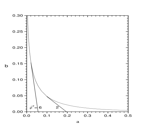
FIG. 1.: The semiclassical boundary of the stability region for stable strings in the $(a,b)$ plane. The square $\bar{\rho}^{2}$ of the thickess of some solutions is also shown.

and for small enough $1/m_{H}$ and $\delta$ to satisfy conditions (28), a stable solution exists. For a given $\nu$ it is a small deformation of the twisted $Q=1$ Belavin-Polyakov configuration with size $\bar{\rho}$ as shown on the corresponding tangent to the curve. Its energy per unit length is guaranteed by (28) to differ only slightly from $E_{0}=2\pi m_{H}^{2}/\lambda$. The precise meaning of inequalities (28), as well as the computation of the lower bound on $m_{H}$ and of the upper bound on $\delta$ for a stable solution to exist corresponding to a given point $(a,b)$ in the stability region are dynamical questions dealt with numerically in the following sections.

II Numerical results

A String texture

In this subsection we shall perform a detailed numerical study of the string texture solutions of (2) in order to verify and extend the analytical semiclassical results reviewed briefly above. We find it convenient to start with $\delta=0$ and leave the more general case for a later section.

The ansatz

We use the most general static ($\partial/\partial t=0$), $x_{3}-$independent ($\partial/\partial{x_{3}}=0$), axially symmetric ansatz for an infinite straight string with winding $Q$ stretched along the $x_{3}-$axis

 

$${\Phi=f(\rho)e^{iQ\theta}\;}$$

  (30)

with $\rho$ and $\theta$ the usual polar coordinates in the transverse plane. For static configurations the $Z_{0}$ dependent part of the energy density is the sum $(\partial_{i}Z_{0})^{2}+m^{2}Z_{0}^{2}+e^{2}|\Phi|^{2}Z_{0}^{2}$ of three positive terms minimized for $Z_{0}(\rho)=0$. Similarly, $Z_{3}(\rho)=0$ and $Z_{\rho}(\rho)=0$. Note that constraint (8) and current conservation are automatically satisfied by the ansatz.

The energy density and the current of the ansatz in terms of the rescaled quantities, for which we keep the same symbols, are

 

$${{\cal E}}$$

  (31)

and

$$J_{\theta}=-{\tilde{g}}\Bigl{(}{Q\over\rho}-{\tilde{g}}K(\rho)\Bigr{)}f^{2}$$ (32)

respectively, while the magnetic field ${\bf B}\equiv\nabla\times{\bf Z}$ points in the 3-direction and is equal to

$$B_{3}=K^{\prime}+{{K(\rho)}\over\rho}$$ (33)

Extremizing the energy functional one is led to the following field equations for the unknown functions $f$, $G$ and $K$:

 

$${{}-(K^{\prime}+{K\over\rho})^{\prime}-{\tilde{g}}({{Q}\over\rho}-{\tilde{g}}K)f^{2}+K=0}$$

  (34)

It may be checked that they coincide with equations (5) and (6) evaluated for the ansatz.

The boundary conditions

As usual, finiteness of the energy and the field equations are used to determine the boundary conditions. It is straightforward to check that in the present case of vanishing $\Phi$-mass and twist, the solution at infinity behaves like

 

$${f(\rho)\sim C_{1}/\rho^{Q}\;,}$$

  (35)

while specifically for $Q=1$, the case of interest below, its behaviour at the origin is

$$f(\rho)\sim C_{2}\rho\;,\;\;G(\rho)\sim C_{3}+C_{4}\rho^{2}\;,\;\;K(\rho)\sim{\tilde{g}}C_{2}^{2}\rho$$ (36)

with constant $C_{i}$, $i$=1,2,3 and $C_{4}$ related to $C_{3}$ by $8C_{4}+(m_{H}-C_{3})[2C_{3}(C_{3}+m_{H})+{\tilde{\kappa}}^{2}(C_{3}-m_{H})^{2}]=0$. Consequently, the energy density of a $Q=1$ string behaves as $1/\rho^{4}$ at large distances.

Numerics - Solution search

To search for string texture solutions of (2) we used a relaxation method [15] with locally variable mesh size and the convenient set of boundary conditions

$$f(0)=0\;,\;\;K(0)=0\;,\;\;(\rho f^{\prime})(0)=0$$ (37)

$$G(\infty)=m_{H}\;,\;\;(\rho G^{\prime})(\infty)=0\;,\;\;B_{3}(\infty)=0$$ (38)

following from (35) and (36). One starts with an initial trial configuration, which is iteratively improved until it becomes a solution of the field equations within satisfactory accuracy. As an extra check of the accuracy of the solutions obtained, we used three virial conditions, whose general form we shall describe in the next section. Typically they were satisfied within one part in $10^{3}-10^{4}$. Finally, to make sure that the solutions correspond to local minima of the energy and are stable, we perturbed slightly each one of them, using a large number of smooth random perturbations and verified that the perturbed configurations were always of higher energy.

As explained in the previous section, stable solutions are not expected to exist in an arbitrary model (2), but only in those with parameters within the stability region. Using the semiclassical results to guide the search, one starts with a choice of $(a,b)$ in the stability region. The tangent to the thick curve that passes through $(a,b)$ corresponds to a size value $\bar{\rho}(a,b)$. According to the semiclassical analysis a stable solution should exist, which is a small deformation of (15) with size $\bar{\rho}(a,b)$, provided all conditions (28) are satisfied. Figure 1 shows that $\bar{\rho}$ lies typically between one and five, while $a$ and $b$ are smaller than one. Thus, to satisfy the third constraint in (28)

$${\tilde{g}}m_{H}=\sqrt{{2\over b}}{1\over{m_{H}}}\ll 1$$ (39)

one should take

$$m_{H}\gg\sqrt{{2\over b}}$$ (40)

All remaining conditions are then automatically satisfied. A general remark which follows from the semiclassical analysis is that models with parameters in the upper left corner of Figure 1 favour the existence of thick strings, with the constraints satisfied for relatively low Higgs masses. On the other hand, to find thin strings, one has to search in models with large Higgs mass, and parameters in the lower right corner of Figure 1.

To summarize, the theory with a given set of values of $(a,b)$ in the stability region, and $m_{H}$ satisfying (40), should have a stable solution close to (15) with size $\bar{\rho}(a,b)$. The values of the couplings ${\tilde{g}}$ and ${\tilde{\kappa}}$ follow from $a$, $b$ and $m_{H}$. Accordingly, a good guess for the initial configuration necessary for our numerical procedure is configuration (15) for the scalars and vanishing gauge fields.

Results

We start with the verification that stable solutions exist. We restrict ourselves throughout to the most interesting case $Q=1$.

Applying the recipe of the previous paragraph, choose $a$=0.001, $b$=0.2 and $m_{H}=4$. They correspond to ${\tilde{g}}\simeq 0.2$, ${\tilde{\kappa}}\simeq 0.006$. The profile of the stable texture obtained with an initial configuration with $\bar{\rho}=6.7$ is shown in Figure 2. We have been able to go deeper inside the upper left corner of Figure 1 and find stable string texture for $m_{H}$ as low as two.

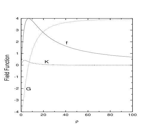
FIG. 2.: The profile of the string in the model with ${\tilde{g}}=0.2$, ${\tilde{\kappa}}=0.006$ and $m_{H}=4$. Its energy is $E=13.6\times 4\pi$.

Similarly, Figure 3 presents the profile of the solution for $a$=0.25, $b$=0.01 and $m_{H}=20$. It corresponds to the model with ${\tilde{g}}=0.04$ and ${\tilde{\kappa}}=0.02$.

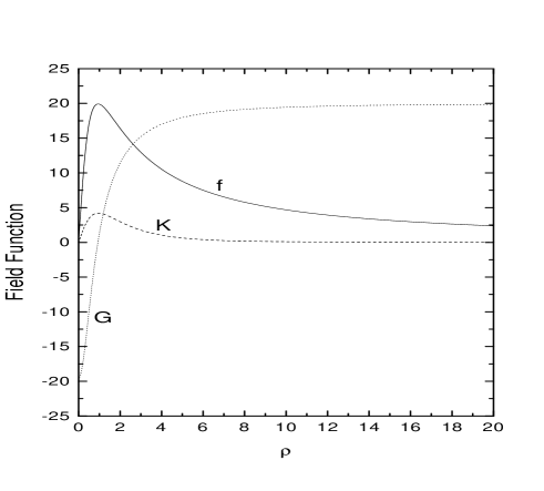
FIG. 3.: For parameters in the lower right corner of Figure 1 stable solutions require larger $m_{H}$ and are thinner.

For both solutions presented above the value of ${\tilde{g}}m_{H}\simeq 0.8$. Thus, the constraint (39) should in practice be interpreted roughly as ${\tilde{g}}m_{H}<1$. Notice that like in the wall case [4] all string solutions discussed here have energies per unit length smaller and within 20% from the value $4\pi m_{H}^{2}$ corresponding to the limiting Belavin - Polyakov solution.

In Figure 4 we plot the Higgs magnitude $F(\rho)\equiv\sqrt{f^{2}+g^{2}}$, the magnetic field $B_{3}$ and the current $J_{\theta}$ for the second solution.

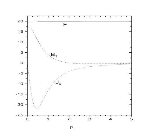
FIG. 4.: The profiles of the Higgs magnitude (solid line), the magnetic field (dashed) and the current (dotted) of the string texture of Figure 3.

Note that the Higgs magnitude differs, in accordance with the theoretical analysis, only slightly from its vacuum value $m_{H}$. Furthermore, it is everywhere non-zero, so that the unit vector field $n_{a}\equiv\Phi_{a}/F$ is well defined and the corresponding winding number (14) unambiguous. Finally, it should be pointed out that the magnetic field takes both positive and negative values. One may verify that the total magnetic flux is zero, as expected from the asymptotic behaviour of the gauge field in (35).

For fixed values of $a$=0.02 and $b$=0.05 we find solutions for a variety of $m_{H}=10,20,30,50$. Their sizes (defined approximatelly for the purposes of this plot by the zero of $G(\rho)$) are plotted in Figure 5 against $m_{H}$ and shown to be roughly constant in accordance with the semiclassical analysis.

For very large $m_{H}$ though one expects deviations from this result. According to Appendix I the thickness of the solutions should eventually increase with $m_{H}$ and for very large Higgs mass be pushed to infinite size. No stable string exists for zero gauge boson mass.

Our next task is to perform a numerical study of the extent of the stability region in the $(a,b)$ plane and compare it against the semiclassical result. We were unable to find stable texture for parameters $(a,b)$ lying above the dashed curve in Figure 6. Notice the remarkable agreement with the leading order semiclassical curve also depicted for convenience by the solid line.

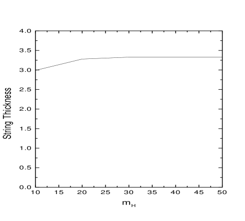
FIG. 5.: For fixed $a$ and $b$ the thickness of the string is rather insensitive to the value of $m_{H}$.

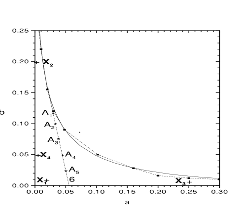
FIG. 6.: The stability region as determined numerically (dashed line) plotted together with the semiclassical result (solid curve).

Finally, it is interesting to test the semiclassical prediction that an infinite set of theories, characterized by parameters on a line of fixed $\bar{\rho}$, all lead to string solutions of the same thickness. The sizes of the solutions obtained for the theories corresponding to the points $A_{1}$ to $A_{5}$ on the line of Figure 6 corresponding to $\bar{\rho}\simeq\sqrt{6}$ are plotted in Figure 7. The Higgs mass was chosen in such a way that the quantity ${\tilde{g}}m_{H}$ is constant and equal to 0.5.

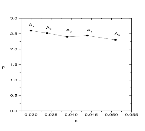
FIG. 7.: The sizes of the string solutions for parameter values corresponding to the points $A_{1}$ to $A_{5}$ of Figure 6, plotted against $a$.

B Twisted strings - Wire quality

Next, we shall extend the previous results and search numerically for current-carrying string texture. We take the string, preferably thought of as a long straight piece of a large loop, stretching along the $x_{3}$-axis and generalise the axially symmetric ansatz used in the previous section, to include a twist in the complex scalar along $x_{3}$

 

$${{}\Phi=f(\rho)e^{iQ\theta}e^{iu(x_{3})}\,,\;\;\Phi_{3}=G(\rho)}$$

  (41)

The gauge current flowing along the string is given by $J_{3}=-g(du/dx_{3}-gW(\rho))f^{2}$. Its conservation translates into ${{d^{2}u(x_{3})}/{dx_{3}^{2}}}=0$ that is, to a linear dependence of the phase $u(x_{3})$ upon $x_{3}$. We shall take the scalar phase to make $N$ full turns over the length $2\pi R$ of the string, and set the constant term to zero. This fixes

$$u(x_{3})={N\over R}x_{3}\equiv\nu x_{3}$$ (42)

In terms of the rescalled dimensionless fields and coordinates defined in the previous section and conveniently denoted by the same symbols, the energy density of the ansatz is:

 

$${{\cal E}}$$

  (43)

Correspondingly, the $x_{3}$-component of the gauge current becomes

$$J_{3}=-{\tilde{g}}\Bigl{(}\nu-{\tilde{g}}W(\rho)\Bigr{)}f^{2}$$ (44)

Extremizing the energy (43) one obtains the field equations

$$-(K^{\prime}+{K\over\rho})^{\prime}-{\tilde{g}}({{Q}\over\rho}-{\tilde{g}}K)f^{2}+K=0$$ (45)

$$-{1\over\rho}(\rho W^{\prime})^{\prime}-{\tilde{g}}(\nu-{\tilde{g}}W)f^{2}+W=0$$ (46)

 

$${-{1\over\rho}(\rho f^{\prime})^{\prime}+({Q\over\rho}-{\tilde{e}}K)^{2}f+}$$

  (47)

 

$${-{1\over\rho}(\rho G^{\prime})^{\prime}+(f^{2}+}$$

  (48)

which we shall solve numerically for fixed non-zero $\nu$, following the same approach as in the previous section.

The boundary conditions.

Finiteness of the energy forces the configuration to tend to the vacuum at spatial infinity . A convenient set of conditions there is given by (36) together with

$$W(\infty)=0$$ (49)

At the center on the other hand we keep (35) and add

$$(\rho W^{\prime})(0)=0$$ (50)

for $W(\rho)$.

Configuration (41), viewed as a circular loop and with the above boundary conditions which effectively compactify space into $S^{3}$, defines a map from $S^{3}$ onto $S^{2}$, the target space of the unit-vector field (12), which as explained before is well defined for all solutions of interest in this paper. As such it is characterised by the Hopf topological index

$$H={1\over{8\pi}}\int_{S^{2}}\epsilon_{abc}\Phi_{a}d\Phi_{b}d\Phi_{c}=Q\cdot N$$ (51)

Notice that for $Q=1$ one may interpret $\nu/2\pi$ as the Hopf charge per unit string length.

An upper bound on the twist magnitude.

It is instructive to view the twisted string as a small deformation of the untwisted one. For $\nu=0$ the $W$-equation gives $W=0$ and the problem reduces to the untwisted case discussed in the previous section. Consider such a stable string corresponding to parameters inside the stability region and to a value of $m_{H}$ not exceeding say 20, to stay near the phenomenologically interesting regime. Start increasing $\nu$, while keeping $\tilde{\kappa}$, $\tilde{g}$ and $m_{H}$ fixed. During this process $b$ in (29) stays fixed, while $a$ increases. Eventually, at some critical value $\nu_{C}$, one will cross the solid curve of Figure 1 and the string solution will disappear altogether . $\nu_{C}$ depends on the values of the other parameters. To maximize the current one should arrange for the maximum relevant value $a_{max}$ of $a$ within the stability region of Figure 1. This corresponds to the lowest value of $b$, which as a consequence of (40) cannot for $m_{H}<20$ exceed the value $b_{min}\simeq 0.01$. Figure 1, then leads to an $a_{max}\simeq 0.3$, which according to (29) translates into ${\Delta}_{max}^{2}/{\tilde{g}}^{2}\simeq 0.3$. Combined with the constraint (39) on the value of ${\tilde{g}}m_{H}$ we obtain

$$\delta_{max}\simeq 0.2$$ (52)

Thus, the maximum current one may hope to drive through such a string corresponds to a twist $\nu_{max}=0.2$. Similarly, according to (52) the value 0.2 is also an estimate of the upper bound on the charged Higgs mass, consistent with the existence of stable strings. String texture corresponding to $m_{H}\geq 20$ may of course support stronger currents and allow for larger $\mu$. In any case, given that according to our analysis, the effects of non-zero $\mu$ and $\nu$ are identical to a high degree of accuracy, we set $\mu=0$ throughout the numerical study that follows.

Virial relations.

Three virial conditions were used to check the accuracy of the solutions discussed in this paper. They express the stationarity of the energy functional under particular deformations of the solution. By the standard argument, imagine a solution of the field equations was found. It is an extremum of the energy. Any small change of the configuration should have to linear order the same energy as the original one. The derivative of the energy functional with respect to the parameters parametrizing the deformation should vanish when evaluated at the solution. The virial conditions we used are

$$E_{1}-2E_{2}=0$$ (53)

$$E_{1}-2E_{3}=0$$ (54)

and

$$2E_{4}-E_{5}=0$$ (55)

relating

$$E_{1}={\pi\over\lambda}\int_{0}^{L}d\rho\;Q\;{\tilde{g}}\;f^{2}\;K$$ (56)

 

$${E_{2}=}$$

  (57)

$$E_{3}={\pi\over{2\lambda}}\int_{0}^{L}d\rho\;\rho\Bigl{[}(K^{\prime}+{K\over\rho})^{2}+(1+{\tilde{g}}^{2}f^{2})\;K^{2}\Bigr{]}$$ (58)

$$E_{4}={\pi\over{4\lambda}}\int_{0}^{L}d\rho\;\rho f^{4}$$ (59)

and

 

$${E_{5}={\pi\over{2\lambda}}\int_{0}^{L}}$$

  (60)

They arise by demanding stationarity of the energy with respect to solution size rescalling $\rho\to\alpha\rho$, $K$-rescalling $K(\rho)\to\beta K(\rho)$ and $f$-rescalling $f(\rho)\to\gamma f(\rho)$, respectively. Such field rescallings are consistent, as they ought to, with the boundary conditions on the fields $K$ and $f$.

All solutions obtained numerically satisfied the above virial conditions to a very good approximation. Specifically, in all cases the appropriately normalized virial quantities $v_{1}=|(E_{1}-2E_{2})/(E_{1}+2E_{2})|$, $v_{2}=|(E_{1}-2E_{3})/(E_{1}+2E_{3})|$ and $v_{3}=|(2E_{4}-E_{5})/(2E_{4}+E_{5})|$ were of ${\cal O}(10^{-4}-10^{-3})$.

Results.

To find twisted solutions we start with an untwisted one as initial trial configuration, and iteratively improve it until it becomes a solution of (45)-(48) with the given value of $\nu$.

Figure 8 shows the profile of the solution arising by the above method from the untwisted string corresponding to point $X_{1}$ with $a=0.02$ and $b=0.01$ in Figure 6. For the remaining parameters we chose $m_{H}=20$ and $\nu=0.05$. As for the initial ansatz we took the Belavin-Polyakov soliton with $\bar{\rho}=3.5$ and vanishing gauge fields.

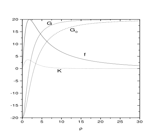
FIG. 8.: The twisted string for ${\tilde{g}}=0.035$, $\tilde{\kappa}=0.005$, $m_{H}=20$ and $\nu=0.05$. On the same plot we also show the profile of the function $G_{0}(\rho)$ of the untwisted solution. The twist reduces string thickness.

To observe the destabilization of the string solution caused by a large current and to determine the value $\nu_{max}$ of the twist, we continued increasing $\nu$ for fixed values of the remaining parameters. For the solution corresponding to $X_{1}$ presented in Figure 8 we found $\nu_{C1}\simeq 0.1$. In a similar fashion, we computed the maximum currents supported by the untwisted string textures plotted in Figures 2 and 3, whose corresponding $(a,b)$ are shown in Figure 6 by the points $X_{2}$, $X_{3}$ and $X_{4}$. The maximum values of the twist found are $\nu_{C2}\simeq 0.01$, $\nu_{C3}\simeq 0.04\;{\rm and}\;\nu_{C4}\simeq 0.04$, respectively. The agreement of these results with the semiclassical absolute bound (52) obtained above is rather satisfactory. The corresponding total current, roughly equal to $I\sim\pi\bar{\rho}^{2}{\tilde{g}}\nu m_{H}^{2}$, is less sensitive. It was evaluated numerically and shown to take values between 30 and 52 for the above solutions. The most promising region of parameters for the existence of stable closed loops is around $X_{1}$, but still $\nu$ cannot easily become large enough to satisfy (1).

C Large string loops

An interesting question, that needs to be addressed in the context of our toy model, is the question of spring formation [12], [16]. The analysis so far does not allow much hope that stable string loops can exist in (2). The semiclassical prediction (52) or even worse the numerically determined maximum value of the twist are much smaller than the value (1) required for spring formation. In fact the last semiclassical constraint in (28), even when interpreted as a simple inequality as suggested by all numerical results obtained above, leaves little room if at all for stable loops. Furthermore, one should note that (1) is rather optimistic for our toy model, because it was obtained for massless gauge field which maximizes the magnetic pressure due to the trapped magnetic flux.

In any case, proper numerical search for string loops in this model would then mean to look for rather small loops with inner radius of the order of the gauge field inverse mass or less, in order to maximize the effect of the gauge field against loop contraction. This requires essentially full three dimensional analysis and was left for a future publication.

However, within the numerical approximation used in this paper, we did verify the above conclusions for large loops of radius $R\gg\bar{\rho}$. We approximated the loop by a straight string of length $2\pi R$ and looked for minima of the energy

$$E(R)=\int_{0}^{2\pi R}dz\int_{0}^{R}d\rho\,\rho\,{\cal E}(f,G,K,W)$$ (61)

to check whether the $R$-dependent term $(N/R-{\tilde{g}}W)^{2}f^{2}$ in the integrand (43), which for fixed $N$ acts against loop contraction, might actually stabilize it at some $R=R_{spring}$.

Clearly, keeping $N$ constant, spring formation could occur only for $R$ large enough so that the solution exists i.e. $N/R=\nu<\nu_{C}\equiv N/R_{C}$ corresponding to the chosen values of the parameters. If this minimum of the energy could be achieved at some $R_{spring}>R_{C}$ then at the $R_{C}(m_{H})$, $E(R)$ would have a negative derivative with respect to $R$ i.e. the total energy $E$ would tend to decrease towards its minimum as $R$ increased from $R_{C}$ towards $R_{spring}$. We have checked all points at $R_{C}$s for a wide range of parameters ($4<m_{H}<1000$, $0<{\tilde{g}}<0.5$, $0<{\tilde{\kappa}}<0.5$) in regions where solutions exist. We focused on regions where $R_{C}$ could be minimized (large $m_{H}$) thus maximizing the twist induced pressure of the $R$-dependent term $(N/R-{\tilde{g}}W)^{2}f^{2}$. It is this term that could potentially stabilize the closed loop. We found that $(dE/dR)|_{R=R_{C}}>0$ at all points with practically no signs of change even at the smallest $R_{C}$’s. Therefore, in line with the previous discussion, we conclude that for the parameter sectors we investigated no spring solutions exist.

III Discussion

To summarize, we have found stable current-carrying vortex solutions in gauged generalizations of the $O(3)$ non-linear $\sigma$-model, with a single $U(1)$ gauge field and the usual scalar triplet. The model considered is an extension of that studied in [7], and may also be viewed as semilocal [2]. Indeed, it has generically a trivial vacuum manifold, while its target space should effectively be thought of as an $S^{2}$ with an $S^{1}$ gauged by the $U(1)$ gauge field. In this model we have mapped the parameter sectors where stable solutions exist, while no stabilized spring solutions were found in the parameter sectors discussed. The parameter region corresponding to stable untwisted string texture [7] has also been examined and we confirmed numerically the approximate semi-analytical results of that analysis. An alternative way to stabilize vortex loops is the introduction of angular momentum whose conservation can stabilize loops against collapse more effectively than twist pressure. Loops stabilized by angular momentum are known as vortons [17] in order to be distinguished from springs.

It is instructive at this point to examine what the above results, obtained in the context of the toy model (2), suggest about the two Higgs-doublet standard model. As mentioned before, the gauge field in (2) corresponds to the $Z^{0}$ gauge boson, while the role of $\Phi$ is here played by the charged Higgs $H^{+}$. Clearly, the numerical results of the present paper strengthen our confidence to the semiclassical conclusions reported in [8], which should be valid with high accuracy. In addition, the constraints are weeker and should be interpreted as simple inequalities. Thus, the 2HSM supports stable strings. They may be generalized and allow for a current to flow along them. The current due to the twist of the electrically charged $H^{+}$ is a bona-fide electric current and the string texture in this case is a superconducting wire in the standard sense. It is characterized by the twist parameter $\nu$, the Hopf charge per unit string length. Being of electroweak scale these ”wires” should have a thickness of a few $m_{W}^{-1}$ and mass density of the order of $10^{-4}gr/cm$. Extrapolating naively to the 2HSM the bounds obtained above, one is led to a maximum current they can carry of about $10^{8}-10^{10}$Amp${\grave{e}}$res, corresponding to $\nu=\nu_{max}\sim 0.2$. Equivalently, these bounds would imply the absence of stable string texture for $H^{+}$ mass $\mu$ larger than $\mu_{max}\sim 0.2m_{Z}\sim 18GeV/c^{2}$. Since this value is lower than the experimental lower bound on the $H^{+}$ mass, little space is left for stable string texture in the 2HSM for realistic values of its parameters.

But, this last conclusion may well be too naive. The presence in general of a separate coupling for electromagnetism and of a richer variety of charged and neutral fields, will change the maximum current allowed along the string, as well as condition (1), derived for the case of the single gauge field of the toy model studied in the present paper. What actually happens in more complicated models like the 2HSM is a matter of detailed analysis and deserves further study.

ACKNOWLEDGMENTS This work is partly the result of a network supported by the European Science Foundation (ESF). The ESF acts as a catalyst for the development of science by bringing together leading scientists and funding agencies to debate, plan and implement pan-European initiatives. This work was also supported by the EU grant CHRX-CT94-0621, as well as by the Greek General Secretariat of Research and Technology grant $\Pi$ENE$\Delta$95-1759.

APPENDIX I

A massless U(1) gauge field does not lead to stable texture. A massless gauge field is either too efficient in halting the shrinking caused by the potential terms and blows-up the texture to infinite thickness, or it is not efficient and the string contracts to vanishing cross section.

Here we sketch a semiclassical proof valid for thick strings. More generally, the statement has been verified numerically. It was shown in the main text that the introduction of either mass or twist to the charged scalar works against the stability of the string texture. It suffices to prove the statement for massless charged scalar and vanishing twist. Start from (2) with $m=\mu=0$. Define the Higgs mass $\sqrt{2\lambda}v=1$ to set the mass scale and rescale fields and distances according to:

$$F\to vF\;,\;\;A_{\mu}\to vA_{\mu}\;,\;\;x^{\mu}\to x^{\mu}/\sqrt{2\lambda}v$$ (62)

after which the action is written as

 

$${{}{\cal L}_{m=0}={v\over{\sqrt{2\lambda}}}\Bigl{[}{1\over 2}(\partial_{\mu}F)^{2}+{1\over 2}F^{2}|(\partial_{\mu}+i{\tilde{g}}A_{\mu})(n_{1}+in_{2})|^{2}}$$

  (63)

with fields and parameters defined as in the main text. Here we have only changed to $A_{\mu}$ the name of the gauge field.

In the limit

$${\tilde{g}},{\tilde{\kappa}}\to 0$$ (64)

the model has absolutely stable topological strings (15) with $F=1$. What will happen to such a soliton of arbitrary size $\bar{\rho}$ if we move slightly away from the limit? Switching-on the potential term will tend to shrink it, while a non-vanishing gauge coupling will tend to blow it up.

Following the steps of [7] it is straightforward to solve for the magnitude $F$ and the gauge field, and derive an effective action for the unit-vector field $n_{a}$. Under the constraints

$$\bar{\rho}\gg 1\;,\;\;{\tilde{\kappa}}\bar{\rho}\ll 1\;,\;\;\tilde{g}\ll 1$$ (65)

the energy per unit length is written as ${\cal E}=E_{0}+\delta{\cal E}$ with

$$E_{0}={v\over\sqrt{2\lambda}}\int d^{2}x{1\over 2}(\partial_{i}n_{a})^{2}$$ (66)

and

 

$${\delta{\cal E}={v\over\sqrt{2\lambda}}\Bigl{[}}$$

  (67)

The current is $J_{i}\equiv{1\over 2}(n_{2}\partial_{i}n_{1}-n_{1}\partial_{i}n_{2})$ and the Green function of the massless gauge field is

$$G_{kl}(x)=\int{{d^{2}p}\over{4\pi^{2}}}e^{-i{\bf p}\cdot{\bf x}}{{\delta_{kl}+p_{k}p_{l}}\over p^{2}}$$ (68)

Following the same steps as in the main text, we evaluate ${\cal E}$ for the solution (15), minimum of the leading term $E_{0}$. The result is

$${\cal E}_{m=0}(\rho)={v\over\sqrt{2\lambda}}4\pi\Bigl{[}1-{8\over{3\bar{\rho}^{2}}}+{1\over{12}}(2{\tilde{\kappa}}^{2}-3{\tilde{g}}^{2})\bar{\rho}^{2}\Bigr{]}$$ (69)

The constant is the leading Belavin-Polyakov value for the $Q=1$ soliton. The remaining terms represent the leading correction to its energy due to the potential and the gauge interaction.

This function does not have a local minimum. Q.E.D.

We should like to point out that this result is quite general in our approximation. Dimensional analysis alone fixes the gauge contribution to the energy to be $\sim Constant\times\bar{\rho}^{2}$. It is ”Lenz” that fixes the coefficient of the quartic term in (67) to be negative. Relaxing the constraint on $F$ reduces the energy of the configuration. Thus, for any value of $Q$ the energy takes the form $\delta E\sim 1-C_{1}/\bar{\rho}^{2}+C_{2}\bar{\rho}^{2}$ with $C_{1}>0$. Independently of the value of $C_{2}$ this function has no local minimum.

For $\Delta\equiv 3{\tilde{g}}^{2}-2{\tilde{\kappa}}^{2}<0$ the gauge repulsion is not strong enough to halt shrinking to zero size. For $\Delta>0$ the energy has a local maximum at $\bar{\rho}_{0}\equiv(4\sqrt{2}/(3{\tilde{g}}^{2}-2{\tilde{\kappa}}^{2}))^{1/4}$. Strings of thickness smaller than $\bar{\rho}_{0}$ shrink to zero, while those of initial thickness larger than $\bar{\rho}_{0}$ blow-up to infinity.

REFERENCES

- [1] C. Bachas and T.N. Tomaras, Nucl. Phys. B428, 209 (1994).
- [2] T. Vachaspati and A. Achucarro, Phys. Rev. D 44, 3067 (1991); M. Hindmarsh, Phys. Rev. Lett. 68, 1263 (1992); A. Achucarro, K. Kuijken, L. Perivolaropoulos and T. Vachaspati, Nucl. Phys. B388, 435 (1992).
- [3] Y. Brihaye and T.N. Tomaras, hep-th/9810061; Nonlinearity 12, 867 (1999).
- [4] C. Bachas and T.N. Tomaras, Phys. Rev. Lett. 76, 356 (1996).
- [5] G. Dvali, Z. Tavartkiladze and J. Nanobashvili, Phys. Lett. 352B, 214 (1995).
- [6] A. Riotto and Ola Tornkvist, Phys. Rev. D56, 3917 (1997).
- [7] C. Bachas and T.N. Tomaras, Phys. Rev. D51, R5356 (1995).
- [8] C. Bachas, B. Rai and T.N. Tomaras, ”New string excitations in two-Higgs-doublet models”, hep-ph/9801263; Phys. Rev. Lett. 82, 2443 (1999).
- [9] C. Bachas, P. Tinyakov and T.N. Tomaras, Phys. Lett. B385, 237 (1996); J. Grant and M. Hindmarch, Phys. Rev D59, 116014 (1999).
- [10] A. Belavin and A. Polyakov, JETP Lett. 22, 245 (1975).
- [11] G. H. Derrick, J. Math Phys. 5, 1252 (1964).
- [12] E. Witten, Nucl. Phys. B249, 557 (1985); J.P. Ostriker, C. Thompson and E. Witten, Phys. Lett. 180B, 231 (1986); R. L. Davis and E.P.S. Shellard, Phys. Lett. B207, 404 (1988); R. L. Davis and E.P.S. Shellard, Phys. Lett. 209B, 485 (1988).
- [13] See for example R. Plonsey and R. Colin, Principles and Applications of Electromagnetic Fields, McGraw-Hill 1961.
- [14] A. Vilenkin and E.P.S. Shellard, in Cosmic Strings and other Topological Defects, Cambridge University Press, 1994.
- [15] W. Press, S. Teukolsky, W. Vetterling and B. Flannery, Numerical Recipes, Chapter 17, Cambridge University Press, 1992.
- [16] E. Copeland, D. Haws, M. Hindmarsh and N. Turok, Nucl. Phys. B306, 908 (1988).
- [17] R. L. Davis, Phys. Rev. D38, 3722 (1988); R. L. Davis and E.P.S. Shellard, Nucl. Phys. B323, 209 (1989); B. Carter, P. Peter and A. Gangui, Phys. Rev. D55, 4647 (1997).