Review on $\alpha_{s}$ at LEP

Abstract

To measure the strong coupling $\alpha_{s}$ from event shape observables two ingredients are necessary. A perturbative prediction containing the dependence of observables on $\alpha_{s}$ and a description of the hadronisation process to match the perturbative prediction with the hadronic data.

As perturbative prediction ${\cal O}(\alpha_{s}^{2})$, NLLA and combined calculations are available. Beside the well known Monte-Carlo based models also analytical predictions, so called power corrections, exist to describe the hadronisation. Advantages and disadvantages of the different resulting methods for determining the strong coupling and its energy dependence will be discussed, the newest Delphi results will be presented, and an overview of the LEP results will be included.

1 INTRODUCTION

The theoretical description of hadron production in $e^{+}e^{-}$-annihilation consists of three parts. The first part is based on the fundamentals of the standard model: Feynman diagrams are used to (perturbatively) calculate the electroweak process of $e^{+}e^{-}$-annihilation and the evolution of partons under the strong interaction. At some stage the partons must be combined to become hadrons. This hadronisation process cannot be described by perturbation theory and thus builds a second (non-perturbative) part. Finally the decay of unstable hadrons, which can be described by kinematics using experimentally measured decay rates, need to be included before the prediction can be confronted with data.

Several different predictions exist for the two first parts. Calculations of the evolution of quarks and gluons are available in fixed order $\cal O$($\alpha_{s}^{2}$), recently some observables became available in $\cal O$($\alpha_{s}^{3}$), and in the next to leading log approximation (NLLA), which resums large logarithms to all orders of $\alpha_{s}$. When combining $\cal O$($\alpha_{s}^{2}$) with NLLA matching ambiguities occur leading to even more competing predictions.

To describe the second part (the hadronisation) usually generator based models are used. The most reliable of these models are the Lund string fragmentation, implemented in Jetset, and the Cluster fragmentation, implemented in Herwig. Recently analytical predictions, so called power corrections, became available to describe the influence of hadronisation on event shape observables.

Given the many different possibilities to determine $\alpha_{s}$ it was necessary to restrict this review due to time and space limitation. I’ve chosen to review the analyses using event shape observables to determine $\alpha_{s}$, as this field currently is very active at LEP.

In the following I will first discuss the standard method for measuring $\alpha_{s}$ from event shapes, which uses $\cal O$($\alpha_{s}^{2}$), NLLA or the combined $\cal O$($\alpha_{s}^{2}$)+NLLA prediction in combination with generator based hadronisation models. In the second part the energy dependence of $\alpha_{s}$ will be discussed introducing the alternative analytic description of hadronisation by power corrections. Finally first results obtained using the new $\cal O$($\alpha_{s}^{3}$) predictions are presented. In all three sections Delphi-analyses shall serve as showcases.

2 CONSISTENT DETERMINATION OF THE STRONG COUPLING

The original motivation of repeating an $\alpha_{s}$-measurement with LEP1 data in Delphi was to include the event orientation, given e.g. by the polar angle of the Thrust axis $\theta_{T}$, into the fit. Second order coefficients including such an event orientation became available in $\cal O$($\alpha_{s}^{2}$) through the Event2 program by Catani and Seymour [1]. Using the fully reprocessed LEP1 data, event shapes were measured very precisely in eight bins of $\theta_{T}$. The small systematic errors result not only from the good quality of the final data reprocessing, but also from the fact that all detector corrections in this measurement were naturally calculated for each $\theta_{T}$-bin separately.

The second order prediction for such distributions now contains second order coefficients $A$ and $B$ which depend on the observables value itself and on $\theta_{T}$:

$$\frac{1}{N}\frac{\mathrm{d}^{2}N}{\mathrm{d}y\,\mathrm{d}\theta_{T}}=A(y,\theta_{T})\frac{\alpha_{s}(\mu)}{2\pi}+\left(A(y,\theta_{T})\cdot 2\pi b_{0}\ln\left(\frac{\mu^{2}}{E_{\mathrm{cm}}^{2}}\right)+B(y,\theta_{T})\right)\left(\frac{\alpha_{s}(\mu)}{2\pi}\right)^{2}$$ (1)

$\mu$ being the renormalisation scale and $b_{0}=(33-2N_{f})/12\pi$. Beside $\alpha_{s}$ this formula contains renormalisation scale $x_{\mu}$ parametrised as $x_{\mu}=\mu^{2}/E_{\mathrm{cm}}^{2}$ as a free parameter.

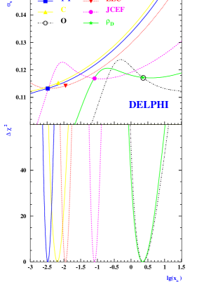
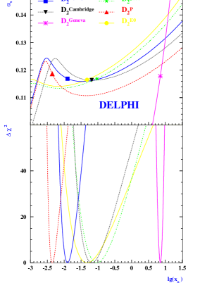
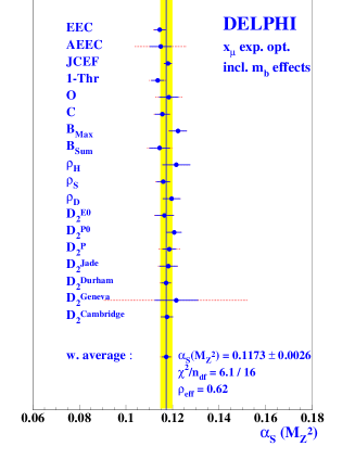
Figure 1: Dependence of the resulting $\alpha_{s}$ on the renormalisation scale for different event shapes (upper parts in left and middle plot) and the corresponding $\Delta\chi^{2}$-values (lower parts). Resulting $\alpha_{s}$ values for 18 different event shape observables using experimentally optimised scale and including corrections for $b$-quark mass (right plot).

As a first step the dependence of the resulting $\alpha_{s}$-values on this parameter were investigated. It is found that different observables aquire largely different dependencies on $x_{\mu}$. Also the scales with the optimal $\chi^{2}/\mathrm{ndf}$ vary widely (see Fig. 1 left and middle). In spite of this large variation of the optimal scale, the $\alpha_{s}$ results corresponding to the experimentally optimised scales show a smaller spread for a large number of different event shapes, than the results obtained with $x_{\mu}=1$. In contrast to the results with scale $1$, optimised scales yield consistent values of $\alpha_{s}$ without assuming any renormalisation scale error (see Fig. 1 right). In addition the scale dependence of $\alpha_{s}$ near the optimised scale is smaller than for $x_{\mu}=1$, so that the scale variation between half and twice the chosen value of $x_{\mu}$ leads to a smaller scale uncertainty for optimised scales.

Averaging over all 18 investigated observables the final result [2] is

$$\alpha_{s}(M_{\mathrm{Z}}) = 0.1228\pm 0.0119\quad\mbox{($x_{\mu}=1$)}$$ (2)

$$\alpha_{s}(M_{\mathrm{Z}}) = 0.1173\pm 0.0026\quad\mbox{(opt. scales),}$$ (3)

where for the optimised scales also the $b$-quark mass corrections are included. The overall fit quality of these results is far better for the optimised scales than for $x_{\mu}=1$, as can be seen from the $\Delta\chi^{2}$ in Fig. 1. Thus the larger spread of the results with $x_{\mu}=1$ can be attributed to a less stable fit procedure which is caused by the bad agreement between data and the prediction.

To crosscheck the results the scale dependence was also investigated for NLLA and combined $\cal O$($\alpha_{s}^{2}$)+NLLA predictions. In contrast to the $\cal O$($\alpha_{s}^{2}$) results the required relative renormalisation scales are close to one and thus there is no significant change compared to the results obtained with $x_{\mu}=1$. Moreover, because of the limited fit range available for NLLA and because of the matching ambiguities for combined $\cal O$($\alpha_{s}^{2}$)+NLLA predictions the total error for these methods is larger than for the $\cal O$($\alpha_{s}^{2}$) result:

$$\alpha_{s}(M_{\mathrm{Z}}) = 0.116\pm 0.006\qquad\mbox{NLLA}$$ (4)

$$\alpha_{s}(M_{\mathrm{Z}}) = 0.119\pm 0.005\qquad\mbox{$\cal O$($\alpha_{s}^{2}$)+NLLA}$$ (5)

Both results are in good agreement with each other and with the $\cal O$($\alpha_{s}^{2}$) results [2].

There are two other publication in which optimised scales are used to determine $\alpha_{s}$ at $E_{\mathrm{cm}}=M_{\mathrm{Z}}$: Already in 1992 Opal [3] states to have found a clear improvement in the fit quality with optimised scales using 14 observables. They quote

$$\alpha_{s}(M_{\mathrm{Z}}) = 0.118^{+0.007}_{-0.003}\quad\mbox{(opt. scales),}$$ (6)

where the error includes a scale variation from the optimised scale upto a scale of 1.

In 1996 Burrows et. al. [4] investigated 15 Observables using SLD-data. In contrast to Opal and Delphi they found no significant reduction of the spread of $\alpha_{s}$-values, though the shift to lower values of $\alpha_{s}$ when using optimised scales is reproduced:

$$\alpha_{s}(M_{\mathrm{Z}}) = 0.1265\pm 0.0076\quad\mbox{($x_{\mu}=1$)}$$ (7)

$$\alpha_{s}(M_{\mathrm{Z}}) = 0.1173\pm 0.0071\quad\mbox{(opt. scales).}$$ (8)

In spite of the extra theoretical uncertainties due to matching ambiguities three of four LEP experiments today use the combined $\cal O$($\alpha_{s}^{2}$)+NLLA calculation to determine their central $\alpha_{s}$-value (second error at L3 is the theoretical component):

$$\begin{array}[]{rcll}\alpha_{s}(M_{\mathrm{Z}})&=&0.1216\pm 0.0039&\quad\mbox{{\sc Aleph}~{}\cite[cite]{[\@@bibref{}{eps-hep99_1-410}{}{}]}}\\ \alpha_{s}(M_{\mathrm{Z}})&=&0.1220\pm 0.0015\pm 0.0060&\quad\mbox{{\sc L3}~{}\cite[cite]{[\@@bibref{}{l3note2414}{}{}]}}\\ \alpha_{s}(M_{\mathrm{Z}})&=&0.120\hskip 5.00002pt\pm 0.006&\quad\mbox{{\sc Opal}~{}\cite[cite]{[\@@bibref{}{ZPhysC55_1}{}{}]}.}\end{array}$$ (9)

3 ENERGY DEPENDENCE

The increase of beam energy accomplished during the LEP2 programme gives access to the energy dependence of event shapes and thereby to the energy dependence of $\alpha_{s}$.

3.1 Power Corrections

Using data at different energies allows also to replace the generator based hadronisation models by an analytical ansatz. For mean values this ansatz (which was developed by Dokshitzer and Webber [7]) describes the hadronisation by an additive term:

$$\left<f\right>=\frac{1}{\sigma_{\mathrm{tot}}}\int f\frac{\mathrm{d}f}{\mathrm{d}\sigma}\mathrm{d}\sigma=\left<f_{\mathrm{pert}}\right>+\left<f_{\mathrm{pow}}\right>\quad\mbox{.}$$ (10)

The 2nd order perturbative prediction is given by Eq. (1) with coefficients A and B integrated over $y$ and $\theta_{T}$. The power correction term is falling off like the inverse centre-of-mass energy and is given by

$$\left<f_{pow}\right>=c_{f}\frac{4C_{F}}{\pi^{2}}{\cal M}\frac{\mu_{I}}{E_{\mathrm{cm}}}\left[{\alpha}_{0}(\mu_{I})-\alpha_{s}(\mu)-\left(b_{0}\cdot\log{\frac{\mu^{2}}{\mu_{I}^{2}}}+\frac{K}{2\pi}+2b_{0}\right)\alpha_{s}^{2}(\mu)\right]$$

Observable	${\alpha}_{0}(2\,\mbox{Ge\kern-0.86108ptV})$	$\alpha_{s}(M_{\mathrm{Z}})$	$\chi^{2}/\mathrm{ndf}$
$\left<B_{\mathrm{max}}\right>$	$0.407\pm 0.022\pm 0.055$	$0.117\pm 0.0012\pm 0.0015$	8.28/21
$\left<1-T\right>$	$0.493\pm 0.009\pm 0.006$	$0.119\pm 0.0014\pm 0.0067$	64.0/32
$\left<M_{\mathrm{h}}^{2}/E_{\mathrm{vis}}^{2}\right>$	$0.545\pm 0.023\pm 0.017$	$0.120\pm 0.0020\pm 0.0050$	8.28/21

Table 1: Determination of $\alpha_{0}$ in a combined fit of $\alpha_{0}$ and $\alpha_{s}$ using a large number of measurements [10] at different energies [12]. The first error is calculated from the fit, the second contains the renormalisation scale dependence.

where $\alpha_{0}$ is a non-perturbative parameter accounting for the contributions to the event shape below an infrared matching scale $\mu_{I}$, $K=(67/18-\pi^{2}/6)C_{A}-5N_{f}/9$. The Milan factor ${\cal M}$ is set to 1.8, which corresponds to three active flavours in the non-perturbative region [8]. The observable-dependent coefficient $c_{f}$ is 2 and 1 for $f=\left<1-T\right>$ and $f=\left<M_{\mathrm{h}}^{2}/E_{\mathrm{vis}}^{2}\right>$, respectively. For $\left<B_{\mathrm{max}}\right>$ the coefficient is itself energy dependent: $c_{\left<B_{\mathrm{max}}\right>}\sim 1/\sqrt{\alpha_{s}(E_{\mathrm{cm}})}$ [9]. The infrared matching scale is set to 2 GeV as suggested by the authors [7], the renormalisation scale $\mu$ is set to be equal to ${E_{\mathrm{cm}}}$. Beside $\alpha_{s}$ these formulae contain $\alpha_{0}$ as the only free parameter. In order to measure $\alpha_{s}$ from individual high energy data this parameter has to be known.

To infer $\alpha_{0}$, a combined fit of $\alpha_{s}$ and $\alpha_{0}$ to a large set of measurements at different energies [10] is performed [11, 12]. For $E_{\mathrm{cm}}\geq M_{\mathrm{Z}}$ only Delphi measurements are included in the fit. The resulting values of $\alpha_{0}$ for $\left<B_{\mathrm{max}}\right>$, $\left<1-T\right>$ and $\left<M_{\mathrm{h}}^{2}/E_{\mathrm{vis}}^{2}\right>$ are summarised in Tab. 1. Even though the found $\alpha_{0}$ values are experimentally inconsistent, the universality of $\alpha_{0}$ is not violated because the expected theoretical precision allows deviations of upto 20%. The $\alpha_{0}$ values are consistent with the corresponding analyses of L3 [6] and Opal/Jade [13].

After fixing $\alpha_{0}$ to the values found, $\alpha_{s}$ can be calculated individually for each energy using Eqs. (10–3.1). The results for energies between 65 GeV and 189 GeV of this method and of the traditional methods described in the previous section are compared in Fig. 2. All methods give consistent results.

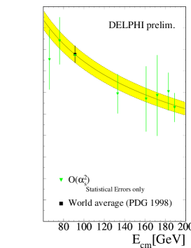
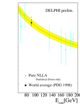
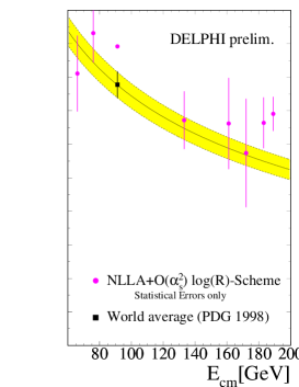
	Power Corr.	Monte Carlo based hadronisation models
	$\cal O$($\alpha_{s}^{2}$)	$\cal O$($\alpha_{s}^{2}$)	NLLA	$\cal O$($\alpha_{s}^{2}$)+NLLA
$\displaystyle\frac{\mathrm{d}\alpha_{s}^{-1}}{\mathrm{d}\log E_{\mathrm{cm}}}$	$1.07$$\pm 0.19\pm 0.20$	$1.23$$\pm 0.31\pm 0.19$	$1.41$$\pm 0.31\pm 0.27$	$1.12$$\pm 0.22\pm 0.18$

Figure 2: Comparison of $\alpha_{s}$-results obtained by Delphi at different centre-of-mass energies using Monte Carlo generator based hadronisation models as well as power correction. Below each plot the result for the logarithmic energy slope of the inverse coupling is given.

3.2 Energy dependence of $\alpha_{s}$

To measure the energy dependence of $\alpha_{s}$ Delphi uses the logarithmic energy slope of the inverse coupling. This quantity is directly proportional to the Callan-Symanzik $\beta$-function and is independent of $\alpha_{s}$ and of $E_{\mathrm{cm}}$ to first order:

$$\frac{\mathrm{d}\alpha_{s}^{-1}}{\mathrm{d}\log E_{\mathrm{cm}}} = -\frac{1}{\alpha_{s}^{2}}\beta_{\alpha_{s}}=\frac{\beta_{0}}{2\pi}+\frac{\beta_{1}}{4\pi^{2}}\alpha_{s}+\ldots\simeq 1.27$$ (11)

The numerical value represents the QCD prediction calculated in second order for energies between 91 GeV and 200 GeV using the PDGs world average of $\alpha_{s}$. The energy dependence of this derivative in the given range and the uncertainty of $\alpha_{s}$ influence this value by about one unit in the last digit.

The result with the smallest systematic error is obtained from $\cal O$($\alpha_{s}^{2}$)+NLLA fits:

$$\frac{\mathrm{d}\alpha_{s}^{-1}}{\mathrm{d}\log E_{\mathrm{cm}}} = 1.12\pm 0.22\pm 0.18$$ (12)

in good agreement with the QCD expectation.

Instead of determining a value for the energy dependence explicitly L3 checks the running of $\alpha_{s}$ by applying a combined fit to all energies assuming the standard model running to $\cal O$($\alpha_{s}^{3}$). This yields a $\chi^{2}/\mathrm{ndf}=15.4/12$ also indicating a good agreement [6].

4 $\cal O$($\alpha_{s}^{3}$)

Third order calculations for four-parton final states have become available recently [14, 15]. These calulations can be used to measure $\alpha_{s}$ in next to leading order from event shapes that acquire non-trivial values only for four and more partons, like the four-jet-rate $R_{4}$:

$$R_{4}=B\left(\frac{\alpha_{s}(\mu)}{2\pi}\right)^{2}+\left(B\cdot 2\pi b_{0}\log\frac{\mu^{2}}{E_{\mathrm{cm}}^{2}}+C\right)\left(\frac{\alpha_{s}(\mu)}{2\pi}\right)^{3}$$ (13)

Observables of this kind are uncorrelated to the observables discussed so far which are based on three-jet-like configurations. The reduced number of relavant events is partly compensated by the (due to quadratic $\alpha_{s}$ dependence) increased sensitivity in Eq. (13).

Delphi investigated four-jets-rates $R_{4}(y_{\mathrm{cut}})$ at a given $y_{\mathrm{cut}}$ for the Durham cluster algorithm [16]. It shows good agreement with the prediction for $y_{\mathrm{cut}}>0.002$. Using $y_{\mathrm{cut}}=0.0025$ the resulting $\alpha_{s}$ values are consistent with the results shown in the previous section, but they have larger statistical errors. Also the running obtained from this analysis is in good agreement:

$$\frac{\mathrm{d}\alpha_{s}^{-1}}{\mathrm{d}\log E_{\mathrm{cm}}} = 1.16\pm 0.46\quad\mbox{.}$$ (14)

This new calculation has also been investigated by Aleph, but was not yet used to determine the strong coupling.

5 SUMMARY

In this talk it was tried to give an overview over the current state of the art in measuring $\alpha_{s}$ from event shape observables at LEP. Beside different perturbative calculations several hadronisation models (generator based and analytical ones) exist. The previous standard choice for the perturbative calculation $\cal O$($\alpha_{s}^{2}$)+NLLA is questioned by Delphi due to poor data description and unsatisfactory consistency.

In that sense measurements of $\alpha_{s}$ from LEP data are still in full progress. In addition to the method used, special attention is payed to tests of the running, also new theoretical developements like power corrections and $\cal O$($\alpha_{s}^{3}$) gain due recognition.

References

- [1] S. Catani and M. H. Seymour Nucl. Phys. B485 (1997) 291–419, hep-ph/9605323.
- [2] DELPHI, EPS-HEP99 # 1_224, 1999.
- [3] OPAL, P. D. Acton et. al. Z. Phys. C55 (1992) 1.
- [4] P. N. Burrows, H. Masuda, D. Muller, and Y. Ohnishi Phys. Lett. B382 (1996) 157, hep-ph/9602210.
- [5] ALEPH ALEPH 99-023, EPS-HEP99 # 1_410, 1999.
- [6] L3, L3 Note 2414, EPS-HEP99 # 1_279, 1999.
- [7] Y. L. Dokshitzer and B. R. Webber Phys. Lett. B352 (1995) 451.
- [8] Y. L. Dokshitzer, A. Lucenti, G. Marchesini, and G. P. Salam Nucl. Phys B511 (1997) 396, hep-ph/9707532.
- [9] Y. L. Dokshitzer, G. Marchesini, and G. P. Salam hep-ph/9812487.
-
[10]
ALEPH Coll., D. Decamp et al. Phys. Lett. B284 (1992) 163.
ALEPH Coll., D. Buskulic et al. Z. Phys. C55 (1992) 209.
AMY Coll., I.H. Park et al. Phys. Rev. Lett. 62 (1989) 1713.
AMY Coll., Y.K. Li et al. Phys. Rev. D41 (1990) 2675.
CELLO Coll., H.J. Behrend et al. Z. Phys. C44 (1989) 63.
HRS Coll., D. Bender et al. Phys. Rev. D31 (1985) 1.
P.A. Movilla Fernandez, et. al. and the JADE Coll. Eur. Phys. J. C1 (1998) 461.
L3 Coll., B. Adeva et al. Z. Phys. C55 (1992) 39.
Mark II Coll., A. Peterson et al. Phys. Rev. D37 (1988) 1.
Mark II Coll., S. Bethke et al. Z. Phys. C43 (1989) 325.
MARK J Coll., D. P. Barber et al. Phys. Rev. Lett. 43 (1979) 831.
OPAL Coll., P. Acton et al. Z. Phys. C59 (1993) 1.
PLUTO Coll., C. Berger et al. Z. Phys. C12 (1982) 297.
SLD Coll., K. Abe et al. Phys. Rev. D51 (1995) 962.
TASSO Coll., W. Braunschweig et al. Phys. Lett. B214 (1988) 293.
TASSO Coll., W. Braunschweig et al. Z. Phys. C45 (1989) 11.
TASSO Coll., W. Braunschweig et al. Z. Phys. C47 (1990) 187.
TOPAZ Coll., I. Adachi et al. Phys. Lett. B227 (1989) 495.
TOPAZ Coll., K. Nagai et al. Phys. Lett. B278 (1992) 506.
TOPAZ Coll., Y. Ohnishi et al. Phys. Lett. B313 (1993) 475. . - [11] DELPHI Coll., P. Abreu et. al. Phys. Lett. B456 (1999) 322.
- [12] DELPHI, EPS-HEP99 # 1_144, 1999.
- [13] OPAL and JADE EPS-HEP99 # 1_5, 1999.
- [14] L. Dixon and A. Signer Phys. Rev. D56 (1997) 4031–4038, hep-ph/9706285.
- [15] Z. Nagy and Z. Trocsanyi Phys. Rev. Lett. 79 (1997) 3604–3607, hep-ph/9707309.
- [16] U. Flagmeyer Talk given at the QCD 99 conference held in Montpellier, July 1999, to be published in Nucl. Phys. (Proc. Suppl.), 1999.