Mesons in non-local chiral quark models

Abstract

After briefly reviewing chiral quark models with non-local regulators and listing their advantages over the conventional Nambu-Jona-Lasionio-like models, we study vector meson correlators in both types of approaches. Since effective chiral quark models are valid in the Eulidean domain only, with $-0.5{\rm GeV}^{2}\leq q^{2}\leq 0$, in our study the meson correlators are not described directly, but with help of a method based on dispersion relations for the physical correlators. A set of sum rules is derived, which allows for a comparison of model predictions to data. We find that both the local and non-local models fail to satisfy the sum rules, unless very low values of the constituent quark mass parameter are used. We also show that the two Weinberg sum rules hold in the non-local model.

This research has been done in collaboration with Maxim Polyakov from Bochum.

I Why non-local regulators?

First, let me recall the reasons why we wish to consider chiral quark models with non-local regulators (see also the contribution by Bojan Golli and Georges Ripka to these proceedings):

1. Non-locality arises naturally in several approaches to low-energy quark dynamics, such as the instanton-liquid model Diakonov86 ; instant1:rev ; instant2:rev or Schwinger-Dyson resummations Roberts92 . For the discussions of various “derivations” and applications of non-local quark models see, e.g.,Ripka97 ; Cahill87 ; Holdom89 ; Ball90 ; Krewald92 ; Ripka93 ; BowlerB ; PlantB ; mitia:rev ; Bijnens . Hence, we should cope with non-local regulators from the outset.

2. Non-local interactions regularize the theory in such a way that the anomalies are preserved Ripka93 ; Arrio and charges are properly quantized. With other methods, such as the proper-time regularization or the quark-loop momentum cut-off mitia:rev ; Bijnens ; Goeke96 ; Reinhardt96 the preservation of the anomalies can only be achieved if the (finite) anomalous part of the action is left unregularized, and only the non-anomalous (infinite) part is regularized. If both parts are regularized, anomalies are violated badly krs ; bbs . We consider such a division artificial and find it quite appealing that with non-local regulators both parts of the action can be treated on equal footing.

3. With non-local interactions the effective action is finite to all orders in the loop expansion ($1/N_{c}$ expansion). In particular, meson loops are finite and there is no more need to introduce extra cut-offs, as was necessary in the case of local models Ripka96b ; Tegen95 ; Temp . As the result, non-local models have more predictive power.

4. As Bojan Golli, Georges Ripka and WB have shown nls , stable solitons exist in a chiral quark model with non-local interactions without the extra constraint that forces the $\sigma$ and $\pi$ fields to lie on the chiral circle. Such a constraint is external to the known derivations of effective chiral quark models.

5. The empirical values of the low-energy constants $g_{8}$ and $g_{27}$ of the effective weak chiral Lagrangian are better reproduced within the non-local model Franz compared to the conventional NJL model.

In view of these improvements it becomes important to look at all other applications of effective quark models and compare the predictions of non-local and local versions.

II Dispersion-relation sum rules for meson correlators

In this talk we will present results for the vector-meson correlators.

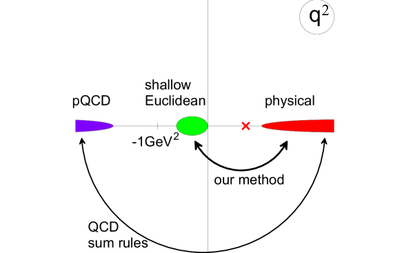
Figure 1:

The basic object of our study is the meson correlation function, defined as

$$\Pi^{AB}(q^{2})=\langle 0|i\int d^{4}x\,e^{iq\cdot x}{\rm T}\left\{j^{A}(x),j^{B}(0)\right\}|0\rangle,$$ (1)

where ${\rm T}$ denotes the time-ordered product, and $j^{A}(x)$ describes a color-singlet quark bilinear with appropriate Lorentz and flavor matrix, e.g. in the $\rho$-meson channel we have $j^{a}_{\mu}(x)=\frac{1}{2}\bar{\psi}(x)\gamma_{\mu}\tau^{a}\psi(x)$. The tensor structure can be taken away, with $\Pi^{AB}(q^{2})=t^{AB}\Pi(q^{2})$, where $t^{AB}$ is a tensor in the Lorentz and isospin indices, and $\Pi(q^{2})$ is a scalar function. The powerful feature of $\Pi(q^{2})$ is its analyticity in the $q^{2}$ variable, which will be used shortly. In Figure 1 we display various regions in the complex $q^{2}$ plane: the positive real axis is the physical region, with poles and cuts corresponding to physical states in the particular channel. In that physical region we have (for certain channels) direct experimental information. Far to the left, at the end of the negative real axis, is the deep-Euclidean region, where perturbative QCD and its operator product expansion can be applied. There is yet another region, close to $0$ on the negative real axis: the shallow-Euclidean region. This is the playground of the effective chiral models. Indeed, the most successful attempt to derive such a model from QCD, namely, the instanton-liquid model, has a natural limitation to that region of momenta instant1:rev ; instant2:rev . More to the point, we believe that all effective chiral quark models should be used in and only in the shallow Euclidean domain. There have been many attempts, however, to apply such models directly to the physical region. In our opinion these are doomed to fail because of the lack of confinement, which is a key player in the physical region. With unconfined quarks, the unphysical $q\bar{q}$ continuum obstructs any model calculation for $q^{2}>(2M)^{2}$, where $M\sim 300-400{\rm MeV}$ is the “constituent” quark mass. For these reasons of principles we always remain with the model at low negative $q^{2}$ Boch ; tensor , and compare to the data via the dispersion relation which holds for the physical correlator. In other words, we bring the physical data to the shallow Euclidean region via the dispersion relation. This is similar in spirit to the QCD sum rule approach, where one compares the physical spectrum to the deep Euclidean region via (Borelized) dispersion relation (see Figure 1).

The correlators considered here satisfy the twice-subtracted dispersion relation

$$\Pi(Q^{2})=c_{0}+c_{1}Q^{2}+\frac{Q^{4}}{\pi}\int_{0}^{\infty}ds\frac{{\rm Im}\Pi(s)}{s^{2}(s+Q^{2})},$$ (2)

where $Q^{2}=-q^{2}$, and $c_{i}$ are subtraction constants. Relation (2) holds for the physical correlators, and does not in general hold for the correlators evaluated in models analyt . For some channels (vector channels) ${\rm Im}\Pi(s)$ is obtained directly from experiment, in other channels we have indirect information only, e.g. from QCD sum rules. Let us take the $\rho$-meson channel, where $j_{a}^{\mu}(x)=\frac{1}{2}\bar{\psi}(x)\gamma^{\mu}\tau_{a}\psi(x)$ and $\Pi_{ab}^{\mu\nu}(Q^{2})=\delta_{ab}(Q^{\mu}Q^{\nu}/Q^{2}-g^{\mu\nu})\Pi_{\rho}(Q^{2})$. The spectral strength in related to the ratio

$${\rm Im}\Pi_{\rho}^{{\rm phen}}(s)=\frac{s}{6\pi}\frac{\sigma(e^{+}e^{-}\rightarrow n\pi)}{\sigma(e^{+}e^{-}\rightarrow\mu^{+}\mu^{-})},\quad n=2,4,6,...$$ (3)

known very accurately from experiment. The spectral strength peaks at the position of the $\rho$-meson pole, and at large $s$ assumes the perturbative-QCD value. For our task it is more convenient to use the simple pole+continuum parameterization of ${\rm Im}\Pi_{\rho}(s)$, such as used e.g. in QCD sum rules. In a given channel the fit has the form

$${\rm Im}\Pi^{{\rm phen}}(s)=\frac{\pi s^{2}}{g^{2}}\delta\left(s-m^{2}\right)+a\,s\,\theta(s-s_{0}),$$ (4)

where $a$ is known from perturbative QCD, and $g$, $m$ and $s_{0}$ are chosen such that the experimental data are reproduced. In the $\rho$-channel we have $a=\frac{1}{8\pi}(1+\alpha_{s}/\pi+...)$, $m=0.77{\rm GeV}$, $g^{2}/(4\pi)=2.36$, and $s_{0}=1.5{\rm GeV}^{2}$ QCD:sum:1 . Since all our calculations will be done in the leading-$N_{c}$ level, we drop the $\alpha_{s}$ correction in $a$.

With the parametrization (4) we readily obtain from (2)

$$\Pi^{{\rm phen}}(Q^{2})=c_{0}+c_{1}Q^{2}+\frac{Q^{4}}{g^{2}(m^{2}+Q^{2})}+\frac{a}{\pi}Q^{2}\log\left(1+\frac{Q^{2}}{s_{0}}\right).$$ (5)

On the other hand, $\Pi(Q^{2})$ can be calculated directly in chiral quark models in the shallow Euclidean space. We denote this model correlation $\Pi^{{\rm mod}}(Q^{2}),$ as want to compare it somehow to $\Pi^{{\rm phen}}(Q^{2})$. One possibility is to Fourier-transform to coordinate space Shuryak93 ; Shuryak93b ; Arriola95b ; JamArr . Here we apply a simpler method, which relies on just Taylor-expanding $\Pi^{{\rm phen}}(Q^{2})$ and $\Pi^{{\rm mod}}(Q^{2})$ in the $Q^{2}$ variable. For the phenomenological correlator we get from Eq. (5)

$$\Pi^{{\rm phen}}(Q^{2})=\sum_{k=1}^{\infty}(-)^{k+1}b_{k}^{{\rm phen}}=c_{0}+c_{1}Q^{2}+Q^{2}\sum_{k=1}^{\infty}(-)^{k+1}\left[\left(\frac{Q^{2}}{m^{2}}\right)^{k}+\frac{a}{k\pi}\left(\frac{Q^{2}}{s_{0}}\right)^{k}\right],$$ (6)

whereas for the model correlator we can write

$$\Pi^{{\rm mod}}(Q^{2})=\sum_{k=1}^{\infty}(-)^{k+1}b_{k}^{{\rm mod}},$$ (7)

with the expansion coefficients $b_{k}^{{\rm mod}}$ yet to be determined. We can now compare the coefficients $b_{k}^{{\rm phen}}$ and $b_{k}^{{\rm mod}}$, and form a set of “sum rules”. With two subtractions in (2) we can start at $k=2$: $b_{k}^{{\rm phen}}=b_{k}^{{\rm mod}}$, $k\geq 2$. With the explicit form (6) this gives

$$b_{2}^{{\rm mod}}=\frac{1}{g^{2}m^{2}}+\frac{a}{\pi s_{0}},\quad b_{3}^{{\rm mod}}=\frac{1}{g^{2}m^{4}}+\frac{a}{2\pi s_{0}^{2}},\quad...$$ (8)

Sum rules for higher values of $k$ are sensitive to the details of the phenomenological spectrum, hence are not going to be of much help.

In some channels the coupling constant $g$ is not well known. We can then eliminate it from Eqs. (8) to obtain

$$m^{2}=\frac{b_{2}^{{\rm mod}}-\frac{a}{\pi s_{0}}}{b_{3}^{{\rm mod}}-\frac{a}{2\pi s_{0}^{2}}},\quad m^{2}=\frac{b_{3}^{{\rm mod}}-\frac{a}{2\pi s_{0}^{2}}}{b_{4}^{{\rm mod}}-\frac{a}{3\pi s_{0}^{3}}},\quad...$$ (9)

Sum rules (8) or (9) can be used to verify model predictions for meson correlators.

III Results for the local model

The model evaluation of meson correlators is well known. At the leading-$N_{c}$ level one has

The diagrams with the dashed line occur only if the coupling constant $G$ is non-zero in a given channel. This is the case of the of the $\sigma$ and $\pi$ channels. In the vector channels they may or may not be present, depending on whether we allow for explicit vector interactions between the quarks.

We first consider the $\rho$-channel in the local NJL model with the proper-time regularization mitia:rev ; Bijnens ; Goeke96 ; Reinhardt96 . After some simple algebra we get

$$b_{2}^{{\rm mod}}=\frac{1}{8\pi^{2}}e^{-M^{2}/\Lambda^{2}}\frac{1}{5M^{2}},\quad b_{3}^{{\rm mod}}=\frac{1}{8\pi^{2}}e^{-M^{2}/\Lambda^{2}}\frac{3(M^{2}+\Lambda^{2})}{140M^{4}\Lambda^{2}},\quad...$$ (10)

where $M$ is the constituent quark mass generated by the spontaneous breaking of the chiral symmetry, and $\Lambda$ is the proper-time cut-off, adjusted such that the pion decay constant has its experimental value, $F_{\pi}=93{\rm MeV}$. Here we work in the strict chiral limit, with the current quark mass set to zero. The results for sum rules (9) are shown in Table 1. We can see that the ratios of phenomenological to model coefficients $b_{2}$ and $b_{3}$ are larger than $1$, and increase rather rapidly with increasing $M$. Thus the sum rules (8) favor lower values of $M$. However, even for such low values as $M=250{\rm MeV}$ the ratios $b_{2}^{{\rm phen}}/b_{2}^{{\rm mod}}$ and $b_{3}^{{\rm phen}}/b_{3}^{{\rm mod}}$ are still significantly above $1$. We conclude that the model is far from satisfying the sum rules (8).

Table 1: $\rho$ channel sum rules in the NJL model with the proper-time regulator ($m=0$, $F_{\pi}=93{\rm MeV}$).

$M$ [GeV]	$\Lambda[GeV]$	$b_{2}^{\rm phen}/b_{2}^{\rm mod}$	$b_{3}^{\rm phen}/b_{3}^{\rm mod}$
0.25	$0.79$	$1.8$	$1.4$
0.3	$0.69$	$2.8$	$3.0$
0.35	$0.65$	$4.2$	$5.7$
0.4	$0.64$	$6.1$	$9.9$

Next, we repeat our calculation for the variant of the model where vector interactions are included Bijnens ; Klimt ; Vogl in the Lagrangian: $-\frac{1}{2}G_{\rho}\left((\bar{\psi}\gamma_{\mu}\tau^{a}\psi)^{2}+(\bar{\psi}\gamma_{\mu}\gamma_{5}\tau^{a}\psi)^{2}\right)$. In that model the formulas for the axial coupling constant of the quark, $g_{A}^{Q}$, and for $F_{\pi}$ read

$$g_{A}^{Q}=\left(1+G_{\rho}\frac{N_{c}M^{2}}{\pi^{2}}\Gamma(0,M^{2}/\Lambda^{2})\right)^{-1},\quad F_{\pi}^{2}=g_{A}^{Q}\frac{N_{c}M^{2}}{4\pi^{2}}\Gamma(0,M^{2}/\Lambda^{2}),$$ (11)

with $\Gamma(0,x)=\int_{x}^{\infty}dt\,e^{-t}/t$. The results are shown in Table 2. We can see that the ratio $b_{2}^{{\rm phen}}/b_{2}^{{\rm mod}}$ decreases as $G_{\rho}$ increases. However, uncomfortably large values of $G_{\rho}$ are needed in order to satisfy the sum rule, i.e. to make $b_{2}^{{\rm phen}}/b_{2}^{{\rm mod}}\sim 1$. The conclusion is that at moderate values of $M$ the model needs very large values of $G_{\rho}$ to describe properly the vector channel.

Table 2: Same as Table 1 with vector interactions included.

	$M=0.3{\rm GeV}$				$M=0.35{\rm GeV}$
$G_{\rho}$ [GeV-2]	$\Lambda[GeV]$	$\frac{b_{2}^{\rm phen}}{b_{2}^{\rm mod}}$	$\frac{b_{3}^{\rm phen}}{b_{3}^{\rm mod}}$	$g_{A}^{Q}$	$\Lambda[GeV]$	$\frac{b_{2}^{\rm phen}}{b_{2}^{\rm mod}}$	$\frac{b_{3}^{\rm phen}}{b_{3}^{\rm mod}}$	$g_{A}^{Q}$
0	$0.69$	$1.8$	$3.0$	$1$	$0.65$	$4.2$	$5.7$	$1$
4	$0.78$	$2.2$	$2.1$	$0.86$	$0.72$	$3.4$	$4.0$	$0.86$
8	$0.91$	$1.6$	$1.4$	$0.72$	$0.81$	$2.5$	$2.8$	$0.72$
12	$1.14$	$1.0$	$1.0$	$0.58$	$0.97$	$1.7$	$1.9$	$0.58$

IV Results for the non-local model

The non-local chiral quark model differs from the local versions in the fact that the interaction vertex carries momentum-dependent factors $r(p_{i})$:

For some more details see the contribution of Bojan Golli and Georges Ripka. We use here the following form of the regulator, $r(p^{2})=1/(1+p^{2}/\Lambda^{2})^{2}$, which is simpler that the instanton-model expression but is known to reproduce well its basic predictions. We use the notation $M_{k}=Mr(k^{2})^{2}$, $D_{k}=k^{2}+$ $M_{k}^{2}$. In the vacuum sector one finds that

$$\frac{1}{G} = 4N_{c}N_{f}\int\frac{d_{4}k}{(2\pi)^{4}}\frac{r(k^{2})^{4}}{D_{k}},\quad\langle\bar{u}u\rangle=\langle\bar{d}d\rangle=-4N_{c}\int\frac{d_{4}k}{(2\pi)^{4}}\frac{M_{k}}{D_{k}},$$ (12)

$$\langle\frac{\alpha_{s}}{8\pi}G_{\mu\nu}^{a}G_{a}^{\mu\nu}\rangle = 4N_{c}\int\frac{d_{4}k}{(2\pi)^{4}}\frac{M_{k}^{2}}{D_{k}},\quad F_{\pi}^{2}=4N_{c}\int\frac{d_{4}k}{(2\pi)^{4}}\frac{M_{k}^{2}-k^{2}M_{k}M_{k}^{\prime}+k^{4}M_{k}^{\prime 2}}{D_{k}^{2}},$$

where the first equation is the stationary point condition, expressing the quark coupling constant via the parameter $M$, the second equation is the quark condensate in the chiral limit, the third is the gluon condensate in the chiral limit, Weiss , and the last one gives the pion decay constant BowlerB ; PlantB in the chiral limit. We use the notation $M_{k}^{\prime}=dM_{k}/dk^{2}$.

There is a complication associated with non-local interactions, namely the Noether currents pick up extra contributions. Furthermore, the transverse parts of these currents are not uniquely determined and their choice constitutes a part of the model. Here we use the so-called straight-line $P$-exponent prescription for gauging the model. For a discussion of this and related issues see Refs. BowlerB ; PlantB ; Bled99 . We then find that

where

$$\Gamma^{\mu}=\gamma^{\mu}-\int_{0}^{1}d\alpha\,\frac{dM(k+\alpha q)}{dk_{\mu}},\quad S^{\mu\nu}=-\int_{0}^{1}d\alpha\int_{0}^{1}d\beta\,\frac{d^{2}M(k+\alpha q-\beta q)}{dk_{\mu}dk_{\nu}}.$$ (13)

It is simple to check that the current is conserved, $q_{\mu}\Pi^{\mu\nu}=0$.

Table 3: Same as Table 1 for the non-local model.

$M[GeV]$	$\Lambda[GeV]$	$b_{2}^{\rm phen}/b_{2}^{\rm mod}$	$b_{3}^{\rm phen}/b_{3}^{\rm mod}$
$0.25$	$1.35$	$1.5$	$1.4$
$0.3$	$1.0$	$1.9$	$2.9$
$0.35$	$0.83$	$2.2$	$3.9$
$0.4$	$0.72$	$2.3$	$3.8$

Coming back to the sum rules (8), we note by comparing Tables 1 and 3 that the results are a bit better in the non-local model. Especially at larger values of $M$, around 350MeV, we gain about a factor of 2. The discrepancy leaves room for such effects as the vector-channel interactions and $1/N_{c}$ corrections, which should be the object of a further study.

The effects of non-localities in currents, as depicted in the figure for $\Pi^{\mu\nu}$, bring about 15 % to the results. More precisely, the calculation with $\gamma^{\mu}$ instead of $\Gamma^{\mu}$ in the vertices (and without the sea-gull term $S^{\mu\nu}$) yields $b_{2}^{{\rm mod}}$ and $b_{3}^{{\rm mod}}$ roughly 15% lower.

V Weinberg sum rules

Now we turn to a more formal aspect of our study. An appealing feature of non-local regulators is that now both Weinberg sum rules hold. The famous sum rules (I) and (II) are:

$$\frac{1}{\pi}\int_{0}^{\infty}\frac{ds}{s}\left[{\rm Im}\Pi_{\rho}(s)-{\rm Im}\Pi_{A_{1}}(s)\right] = F_{\pi}^{2},$$ ()

$$\frac{1}{\pi}\int_{0}^{\infty}ds\left[{\rm Im}\Pi_{\rho}(s)-{\rm Im}\Pi_{A_{1}}(s)\right] = -m\langle\bar{u}u+\bar{d}d\rangle.$$ ()

Whereas (I) holds in all variants of the NJL model, in local models (II) picks up $M$ instead of $m$ on the right-hand side, thus is violated badly. To prove the sum rules in the non-local model we consider the dispersion relation

$$\Pi_{\rho}(Q^{2})-\Pi_{A_{1}}(Q^{2})=\frac{1}{\pi}\int_{0}^{\infty}\frac{ds}{s+Q^{2}}\left[{\rm Im}\Pi_{\rho}(s)-{\rm Im}\Pi_{A_{1}}(s)\right].$$ (14)

No subtractions are necessary. We set $Q^{2}=0$. An explicit evaluation gives

$$\Pi_{\rho}(0)-\Pi_{A_{1}}(0)=4N_{c}\int\frac{d_{4}k}{(2\pi)^{4}}\frac{M_{k}^{2}-k^{2}M_{k}M_{k}^{\prime}+k^{4}M_{k}^{\prime 2}}{D_{k}^{2}},$$ (15)

in which we recognize our formula for $F_{\pi}^{2}$ (12), thus verifying (I). To prove WSR II we multiply both sides of (14) by $Q^{2}$ and take the limit of $Q^{2}\rightarrow\infty$. We find, to the first order in the current quark mass $m$,

$$\lim_{Q^{2}\rightarrow\infty}Q^{2}\left(\Pi_{\rho}(Q^{2})-\Pi_{A_{1}}(Q^{2})\right)=$$

$$\lim_{Q^{2}\rightarrow\infty}Q^{2}\int\frac{d_{4}k}{(2\pi)^{4}}\frac{4N_{c}[M_{k}M_{k+Q}+m(M_{k}+M_{k+Q})]}{D_{k}D_{k+Q}}=$$

$$4N_{c}m\lim_{Q^{2}\rightarrow\infty}Q^{2}\int\frac{d_{4}k}{(2\pi)^{4}}\left(\frac{M_{k}}{D_{k}D_{k+Q}}+\frac{M_{k}}{D_{k}D_{k-Q}}\right)=$$

$$8mN_{c}\int\frac{d_{4}k}{(2\pi)^{4}}\frac{M_{k}}{D_{k}}=-2m\langle\bar{u}u+\bar{d}d\rangle.$$ (16)

In passing from the second to the third line in the above derivation we have used the fact that $M_{p}$ is strongly concentrated around $p=0$, thus we could drop the term with $M_{k}M_{k+Q}$ at $Q^{2}\gg\Lambda^{2}$. By a similar argument in the third line we have replaced $Q^{2}/\left((k\pm Q)^{2}+M_{k+Q}^{2}\right)$ by $1$. Finally, in the last line we have recognized our expression for the quark condensate (12). We note that non-local contributions to the Noether currents are suppressed and do not contribute to (16). Similarly, rescattering diagrams as displayed in the equation for $\Pi^{AB}$ can be dropped. This is because the vertex $\Gamma$ contains the regulator, hence the diagram is strongly suppressed at large $Q^{2}$.

Clearly, the reason for the compliance with the second Weinberg sum rule is the fact that the momentum-dependent mass of the quark becomes asymptotically, in the deep-Euclidean region, just the current quark mass. This is not the case of local models Bijnens ; Dmi , where the mass is constant, and this is why these models violate Eq. (() ‣ V).

VI Final remarks

To end this talk we describe shortly the results for other channels. In the $\omega$-meson channel the model results are, at the leading-$N_{c}$ level, exactly the same as for the $\rho$-channel. In the pseudoscalar and scalar channels we do not know the the corresponding parameter $g$ from experiment, hence we consider sum rules (9). In the pion channel the pion pole entirely dominates the sum rules, i.e. the continuum contribution is negligeable and we get $m_{\pi}^{2}\simeq b_{2}^{{\rm mod}}/b_{3}^{{\rm mod}}\simeq b_{3}^{{\rm mod}}/b_{4}^{{\rm mod}}...$ in both the local and non-local variants of the model. In the $\sigma$-meson channel things are more interesting. Whereas in the local model the sum rules (9) simply give the pole at twice the quark mass, $m_{\sigma}=2M$, in the non-local model the predicted value of $m_{\sigma}$ ranges from 400MeV at $M=300{\rm MeV}$ to 470MeV at $M=450{\rm MeV}$ and is insensitive to the value of the threshold parameter $s_{0}$.

One of us (WB) is grateful to Bojan Golli, Georges Ripka, Enrique Ruiz Arriola and Mike Birse for many useful conversations.

References

- (1) D. I. Diakonov and V. Y. Petrov, Nucl. Phys. B 272, 457 (1986).
- (2) T. Schäfer and E. V. Shuryak, Rev. Mod. Phys. 70, 323 (1998).
- (3) D. Diakonov, in Selected topics in nonperturbative QCD, p.397, talk given at International School of Physics, Enrico Fermi, Varenna, Italy, 27 June - 7 July 1995, hep-ph/9602375.
- (4) C. D. Roberts, in QCD Vacuum Structure (World Scientific, Singapore, 1992), p.114.
- (5) G. Ripka, Quarks Bound by Chiral Fields (Oxford University Press, Oxford, 1997).
- (6) J. Praschifka, C. D. Roberts, and R. T. Cahill, Phys. Rev. D36, 209 (1987).
- (7) B. Holdom, J. Terning, and K.Verbeek, Phys. Lett. B232, 351 (1989).
- (8) R. D. Ball, Int. Journ. Mod. Phys. A5, 4391 (1990).
- (9) M. Buballa and S. Krewald, Phys. Lett. B294, 19 (1992).
- (10) R. D. Ball and G. Ripka, in Many Body Physics (Coimbra 1993), edited by C. Fiolhais, M. Fiolhais, C. Sousa, and J. N. Urbano (World Scientific, Singapore, 1993).
- (11) R. D. Bowler and M. C. Birse, Nucl. Phys. A582, 655 (1995).
- (12) R. S. Plant and M. C. Birse, Nucl. Phys. A628, 607 (1998).
- (13) D. Diakonov, Prog. Part. Nucl. Phys. 36, 1 (1996).
- (14) J. Bijnens, C. Bruno, and E. de Rafael, Nucl. Phys. B390, 501 (1993).
- (15) E. R. Arriola and L. L. Salcedo, Phys. Lett. B450, 225 (1999).
- (16) C. Christov, A. Blotz, H. Kim, P. Pobylitsa, T. Watabe, Th. Meissner, E. Ruiz Arriola, and K. Goeke, Prog. Part. Nucl. Phys. 37, 1 (1996).
- (17) R. Alkofer, H. Reinhardt, and H. Weigel, Phys. Rep. 265, 139 (1996).
- (18) Ö. Kaymakcalan, S. Rajeev, and J. Schechter, Phys. Rev.D31, 1109 (1985).
- (19) A. H. Blin, B. Hiller, and M. Schaden, Z. Phys. A331, 75 (1988).
- (20) E. N. Nikolov, W. Broniowski, C. Christov, G. Ripka, and K. Goeke, Nucl. Phys. A608, 411 (1996).
- (21) V. Dmitrašinović, H.-J. Schulze, R. Tegen, and R. H. Lemmer, Ann. of Phys. (NY) 238, 332 (1995).
- (22) W. Florkowski and W. Broniowski, Phys. Lett. B386, 62 (1996).
- (23) B. Golli, W. Broniowski, and G. Ripka, Phys. Lett. B437, 24 (1998).
- (24) M. Franz, H.-C. Kim, and K. Goeke, preprint RUB-TPII-09/99, Ruhr-University Bochum, hep-ph/9908400.
- (25) C. V. Christov, K. Goeke, and M. Polyakov, Ruhr-Universität-Bochum preprint, hep-ph/9501383.
- (26) W. Broniowski, M. Polyakov, H.-C. Kim, and K. Goeke, Phys. Lett. B438, 242 (1998).
- (27) W. Broniowski, G. Ripka, E. N. Nikolov, and K. Goeke, Z. Phys. A354, 421 (1996).
- (28) M. A. Shifman, A. I. Vainshtein, and V. I. Zakharov, Nucl. Phys. B147, 385, 448, 519 (1979).
- (29) E. V. Shuryak, Rev. Mod. Phys. 65 1 (1993).
- (30) E. V. Shuryak and J. J. M. Verbaarschot, Nucl. Phys. B410 37 and 55 (1993).
- (31) R. M. Davidson and E. Arriola, Phys. Lett. B359 273 (1995).
- (32) M. Jaminon and E. R. Arriola, Phys. Lett. B443, 33 (1998).
- (33) S. Klimt, M. Lutz, U. Vogl, and W. Weise, Nucl. Phys. A516, 429 (1990).
- (34) U. Vogl, M. Lutz, S. Klimt, and W. Weise, Nucl. Phys. A516, 469 (1990).
- (35) D. I. Diakonov, M. V. Polyakov, and C. Weiss, Nucl. Phys. B461, 539 (1996).
- (36) W. Broniowski, INP Cracow preprint 1828/PH, talk presented at the Mini-Workshop on Hadrons as Solitons, Bled, Slovenia, 6-17 July 1999, hep-ph/9909438.
- (37) V. Dmitrašinović, S. P. Klevansky, and R. H. Lemmer, Phys. Lett. B386, 45 (1996).