Stochastic treatment of Disoriented Chiral Condensates
within a Langevin description

Abstract

Applying a microscopically motivated semi-classical Langevin description of the linear sigma model we investigate for various different scenarios the stochastic evolution of a disoriented chiral condensate (DCC) in a rapidly expanding system. Some particular emphasize is put on the numerical realisation of colored noise in order to treat the underlying dissipative and nonmarkovian stochastic equations of motion. A comparison with an approximate markovian (i.e. instantaneous) treatment of dissipation and noise will be made in order to identify the possible influence of memory effects in the evolution of the chiral order parameter. Assuming a standard Rayleigh cooling term to simulate a D-dimensional scaling expansion we present the probability distribution in the low momentum pion number stemming from the relaxing zero mode component of the chiral field. The best DCC signal is expected for initial conditions centered around $\langle\sigma\rangle\approx 0$ as would be the case of effective light ‘pions’ close to the phase transition. By choosing appropriate idealized global parameters for the expansion our findings show that an experimentally feasible DCC, if it does exist in nature, has to be a rare event with some finite probability following a nontrivial and nonpoissonian distribution on an event by event basis. DCCs might then be identified experimentally by inspecting higher order factorial cumulants $\theta_{m}$ ($m\geq 3$) in the sampled distribution.

I Introduction and Motivation

The prime intention for ultrarelativistic heavy ion collisions is to study the behaviour of nuclear or hadronic matter at extreme conditions like very high temperatures and energy densities. One of the major goals, particular at the upcoming RHIC facilities, is to find evidence for a new state of deconfined partonic matter, the quark gluon plasma (QGP) [1]. Besides the confinement-deconfinement transition one also expects a transition of hot hadronic matter, where chiral symmetry is being restored. Lattice calculations of quantum chromodynamics (QCD) give the belief, that both transitions do occur at the same critical temperature $T_{c}$ at vanishing net-baryon densities [2].

The formation of so-called disoriented chiral condensate (DCC) [3] has been considered as the maybe most prominent signature for the restoration of chiral symmetry occuring in the ongoing evolution of the hot matter from the chirally restored to the chirally broken phase. The idea is here that in the course of the evolution of the system from the initially (and only transiently existing) unbroken phase with (the order parameter being) $\langle\bar{q}q\rangle\approx 0$ to the true groundstate with $\langle\bar{q}q\rangle\neq 0$ the pseudo-scalar condensate $\langle\bar{q}{\bf\tau}\gamma_{5}q\rangle$ might assume temporarily non-vanishing values. This misaligned condensate has the same quark content and quantum numbers as do pions and thus essentially constitutes a classical pion field. The subsequent relaxation of this field back to the alignment of the outside vacuum could then lead to an excess of low momentum pions in a single direction in isospin space.

The possible occurrence of a semi-classical and coherent pion field was first raised in a work of Anselm [4] but the idea of forming DCC was made widely known due to Bjorken [5] and Rajagopal and Wilczek [6]. Since then many works appeared on various aspects of DCC formation in heavy ion collisions. As the microscopic physics governing the chiral phase transition is not known well enough, one typically employs effective field theories like the linear $\sigma$-model [6] in order to describe this non-equilibrium phenomenon. On the other hand the description of quantum field theory out of equilibrium is interesting in its own right and thus has given raise to a major attraction for theoretical studies in order to describe the evolution of disoriented chiral condensates [7], like e.g. standard Hartree factorization or large $N_{c}$-expansion methods [8]. Usually these considerations assume an initial state at high temperature in which chiral symmetry is restored by vanishing collective fields. Independent thermal fluctuations in each isospin direction of the $O(4)$ $\sigma$-model are present. This configuration sits on the top of the barrier of the potential energy at zero temperature, so a sudden cooling of the system supposedly brings it into an unstable state. This picture is referred to as the quenched situation [6]. The spontaneous growth and subsequent decay of these configurations would give raise to large collective fluctuations in the number of produced neutral pions compared to charged pions, and thus could provide a mechanism explaining a family of peculiar cosmic ray events, the Centauros [9]. A deeper reason for these strong fluctuations lies in the fact that all pions constituting the classical and coherent field are sitting in the same momentum state and the overall wavefunction can carry no isospin [10].

The proposed quench scenario [6] assumes that the effective potential governing the evolution of the long wavelength modes immediately turns to the classical one at zero temperature. This is a very drastic assumption as the soft classical modes completely decouple from the residual thermal fluctuations at the chiral phase transition temperature. Such an idealized scenario of immediate decoupling might hold effectively if the expansion and the associated cooling of the fireball occurs sufficiently fast [11]. An alternative, the annealing scenario [13], was suggested by Gavin and Müller. They used the one-loop effective potential instead of the classical one including thermal fluctuations. For moderate expansion and cooling it was shown that the system can exhibit longer instable periods and thus should lead even to a stronger enhancement of the soft pionic fields. On the other side, both scenarios assume that the initial fluctuation of the order parameter at the beginning of the DCC formation are centered around zero with a sufficiently small width in a rather ad hoc manner. Preparing the initial configuration with stronger initial fluctuations, no DCC formation has been observed [12]. If the soft field remains in thermal contact with the fluctuations giving raise to the one-loop potential, then one also has to allow for appropriate thermal fluctuations in the initial conditions [14, 15]. The proposed quenched initial conditions within the linear sigma model seem statistically unlikely.

The likeliness of an instability leading potentially to a DCC event during the evolution with a continuous contact with the heat bath of thermal pions was investigated by Biro and one of us by means of simple Langevin equations [16]. There the average and statistical properties of individual solutions were studied with the emphasis on such periods of the time evolution when the transverse mass $\mu_{\bot}$ of the pionic modes becomes imaginary and therefore an exponential growth of unstable fluctuations in the collective fields might be expected. It was found that for different realistic initial volumes individual events of an ensemble lead to sometimes significant growth of fluctuations [16, 17]. Subsequent investigation by us in fact leads to the idea of stochastic formation of DCC for particular special stochastic evolution of the order parameter [18].

This idea is what we want to detail in the present study in more depth. Our main conception is that the order parameter before and after the onset of the chiral phase transition still interacts (dissipatively) with its (nearly) thermal surrounding of thermal (or ‘hard’) pions, which then give raise also to large fluctuations in the evolution. This one can interpret as a breakdown of the standard mean-field approximation. Applying a microscopically motivated semi-classical Langevin description of the linear sigma model we investigate for various different scenarios the stochastic evolution of a single disoriented chiral condensate in a rapidly expanding system assuming a D-dimensional scaling expansion [11, 13, 14, 16]. Our stochastic description will allow for a systematic recording of the statistically possible initial configurations of the order parameter. Furthermore it also describes the nontrivial influence of dissipation and fluctuations on the nonequilibrium evolution and the coherent amplification on the collective pionic zero mode fields during and after the onset of the phase transition.

It remains to answer the important question of how likely particular nonequilbrium evolutions of a statistically generated ensemble will lead to the formation of a ‘large’ DCC-domain, which will depend nontrivially on the initial and subsequent fluctuations suffered by the surrounding in the course of the evolution. For this we calculate the effective pion number contained in the pionic collective field emerging by the rolling down of the chiral fields to its true vacuum values, which by subsequent emission will be freed as low momentum pions. With this number at hand we can make the decision whether accordingly these pions can contribute to an experimentally measurable enhancement of low momentum pions and thus might provide indeed a signal for the occuring chiral phase transition. As it turns out the probability distribution in the pion number contains interesting new information for the characteristics of the non-equilibrium evolution stemming from the relaxing zero mode component of the chiral field. In the interesting cases the to be expected yield in low momentum pions do not follow an usual and simple statistical distribution, but posesses large and nontrivial (non-poissonian) fluctuations. The best DCC signal is expected for initial conditions centered around $\langle\sigma\rangle\approx 0$ as would be the case of effective light ‘pions’ close to the phase transition. By choosing some idealized global parameters for a $(D=)\,$3-dimensional, spherical expansion, our findings show that an experimentally feasible DCC, if it does exist in nature, has to be a rare event with some finite probability following a nontrivial and nonpoissonian distribution on an event by event basis. Comparing with an additional incoherent background the fluctuations in the low momentum pion number might be revealed in the nonvanishing of higher order factorial cumulants $\theta_{m}$ ($m\geq 3$). Admittingly, we have to say that although we do stress a new physical picture our study has still to be seen as a fairly idealized scenario. Nevertheless, we believe that our results are interesting in their own right and should serve as a simplified estimate for the nontrivial late dynamics encountered in an ultrarelativistic heavy ion collision.

In the next section II we describe the linear $\sigma$-model within a Langevin treatment. For this we will first summarize the theoretical ideas behind a semi-classical Langevin description for the soft (i.e. low momentum) fields in thermal quantum field theory. The hard modes are treated as thermal quasiparticles which constitute a surrounding, open heat bath. We then discuss the model introduced in [16] in more depth for simulating the evolution of the order parameter and the collective zero mode pionic fields. The damping term entering the dynamical evolution will be discussed and a systematic recording of the statistically possible initial configurations of the order parameter for finite volumes will be given. The final equations of motion to be used for the dynamical evolution including a D-dimensional scaling expansion for modeling the possible formation of DCC are then stated. As a characteristic for describing the ‘strength’ of a DCC we consider the effective pion number content of the evolving domain. Some particular emphasize will then be put first in section III on the numerical realization of colored noise in order to treat the underlying dissipative and nonmarkovian stochastic equations of motion. This, to the best of our knowledge, is the first numerical treatment of nonmarkovian Langevin equations in thermal quantum field theory and might be of importance for other related topics. A comparison with a standard markovian (i.e. instantaneous) treatment of dissipation and noise will be made. For the later simulations it shows that it is sufficient to consider only the markovian approximation, which is numerically much easier to handle. In section IV we finally present numerical results of the simulation on the evolution of a coherent pionic field. Four different scenarios, annealing or quench with initial conditions governed by effective ‘light’ or physical mass pions, will be investigated. We calculate the pion number for a single domain and the distribution of the pion number, which are the observables relevant to the experimental detection of DCC, and which also will give quantitative predicition on the possibility of forming an experimentally accessible DCC. The unusual distribution in the number of low momentum pions is further analyzed by means of a cumulant expansion. To be more realistic we also take into account an additional incoherent (poissonian) contribution on the production of soft pions. Inspecting the resulting distribution for the low momentum pion number we show that the high order factorial cumulants can still be large. This provides a new signature to identify possible DCC formation. Some conclusions for possible experimental searches are drawn. We close our findings with a summary. In appendix A we give a microscopic derivation of the frequency dependence of the dissipation kernel being employed. Appendix B describes in more detail our strategy for simulating gaussian nonwhite, colored noise for an arbitrary noise kernel. Appendix C gives a brief reminder on the cumulant expansion for statistical distributions.

II Langevin description of linear sigma model

In this section we develop in some more detail the Langevin description of the linear $\sigma$-model introduced in [16, 18]. The starting point is the phenomenological Lagrangian which is given by

$${\cal L}\,=\,\frac{1}{2}\,\partial_{\mu}\phi_{a}\partial^{\mu}\phi^{a}\,-\,\frac{\lambda}{4}(\phi_{a}\phi^{a}-v^{2})^{2}\,+\,H\phi_{0}\,,$$ (1)

where $\phi_{a}=(\sigma,\pi_{1},\pi_{2},\pi_{3})$. We employ the standard parameter $f_{\pi}=93$ MeV for the pion decay constant, $m_{\pi}=140$ MeV for the vacuum mass of the pion and $m_{\sigma}\approx 600$ MeV for the ‘mass’ of the $\sigma$-meson. For the three parameters in (1) one then finds

$$\lambda\,=\,\frac{m_{\sigma}^{2}-m_{\pi}^{2}}{2f_{\pi}^{2}}\approx 20,\,v^{2}=f_{\pi}^{2}-\frac{m_{\pi}^{2}}{\lambda}=(87\,\mbox{MeV})^{2},H=f_{\pi}m_{\pi}^{2}\ =(122\,\mbox{MeV})^{3}.$$ (2)

The linear $\sigma$-model represents an effective chiral theory of the low energy properties of QCD. It can be motivated in more theoretical depth from QCD by the modern methods of the renormalization group [19]. At finite temperature, to leading order in $\lambda$, the thermal fluctuations $\langle\delta\phi^{2}(\vec{x},t)\rangle$ of the pions and $\sigma$-mesons do generate an effective Hartree type dynamical mass giving raise to an effective temperature dependent potential. In the high temperature expansion this results in [20]

$$m_{th}^{2}\,\stackrel{{\scriptstyle(T\gg m_{\pi},m_{\sigma})}}{{\longrightarrow}}\,\frac{\lambda}{4}\left(\frac{N+2}{3}\right)T^{2}\stackrel{{\scriptstyle N=4}}{{\longrightarrow}}\,\frac{\lambda}{2}\,T^{2}\,.$$ (3)

The resulting chiral phase transition is compatible with the expectations of lattice gauge QCD calculations [21]. There exist also convincing theoretical arguments [22] that the chiral phase transition near the critical temperature $T_{c}$ of QCD with two massless quarks lies in the same universality class as an $O(4)$-Heisenberg magnet and thus (in this idealized case of massless quarks) exhibits a true second order phase transition which can be described in the Landau-Ginzburg theory by means of an effective linear $\sigma$-model. In this sense one considers the linear $\sigma$-model as an appropriate realisation of the chiral behaviour of QCD over the whole range in temperature, though the effective parameters near $T\approx T_{c}$ need not really be equivalent to those at $T=0$.

We now address in an intuitive model how one can go beyond the mean field level for the semi-classical chiral collective fields. Our main physical conception will be that the order parameter and the collective fields before and after the onset of the chiral phase transition still interacts (dissipatively) with its (nearly) thermal surrounding of thermal (or ‘hard’) particles. To outline these ideas more conceptually we will first summarize in the following subsection the theoretical reasonings behind a semi-classical Langevin description of the soft, i.e. low momentum fields.

A Equations of motion for long wavelength modes in a heat bath

One of the recent topics in especially nonabelian massless quantum field theory at finite temperature or near thermal equilibrium concerns the evolution and behaviour of the long wavelength modes. These modes often lie entirely in the non-perturbative regime. Therefore solutions of the classical field equations in Minkowski space have been widely used in recent years to describe long-distance properties of quantum fields that require a non-perturbative analysis. A justification of the classical treatment of the long-distance dynamics of weakly coupled bosonic quantum fields at high temperature is based on the observation that the average thermal amplitude of low-momentum modes is large and approaches the classical equipartition limit

$$n(\omega_{\bf p})=\left(e^{\hbar\omega_{\bf p}/T}-1\right)^{-1}\buildrel|{\bf p}|\to 0\over{\longrightarrow}{T\over m^{*}}\gg 1$$ (4)

in the case for a sufficiently small generated dynamical mass $m^{*}\ll T$. On the other hand the thermodynamics of a classical field is only defined if an ultraviolet cut-off $k_{c}$ is imposed on the momentum p such as a finite lattice spacing $a$. In a recent paper [23] it was shown, at least principally, how to construct an effective semi-classical action for describing not only the classical behaviour of the long wavelength modes below some given cutoff $k_{c}$, but taking into account also perturbatively the interaction among the soft and hard modes. The resulting effective action $S_{{\rm eff}}[{\rm soft}]$, which one has to interpret as a stochastic, dissipative action [23, 24], turns out to be complex, leading to a stochastic equation of motion for the soft modes. If the hard modes are already in thermal equilibrium then the evolution of the soft modes is described by a set of generalized Langevin equations - the equations of motion corresponding to the above complex effective action.

We briefly sketch the main strategy following [23] by considering a scalar field with interaction ${\cal L}_{{\rm int}}=\frac{g^{2}}{4!}\,\tilde{\phi}^{4}$. The splitting of the Fourier-components, $\tilde{\phi}(p,t)=\phi(p\leq k_{c},t)\,+\,\varphi(p>k_{c},t)$, leads to the following interaction part in the action

$$S_{{\rm int}}[\phi,\varphi]=-\int_{t_{0}}^{t}\!d^{4}x\,\,\left(\frac{g^{2}}{4!}\varphi^{4}+\frac{g^{2}}{3!}\left(\phi^{3}\varphi+\frac{3}{2}\phi^{2}\varphi^{2}+\phi\varphi^{3}\right)\right).$$ (5)

By integrating out the hard modes up to second order in the interaction, one obtains the effective action (or influence functional) $S_{IF}[\phi,\phi^{\prime}]$ for the soft modes following the Feynman-Vernon approach [25]. Fig. 1 shows the resulting non-vanishing diagrams contributing to $S_{IF}$. The contributions from diagram (a) and (b) are real and generate the Hartree like dynamical mass term. Moreover one notices that Feynman graphs contributing at order ${\cal O}(g^{4})$ (diagrams (c), (d) and (e)) to the effective action contain imaginary contributions. Their real part leads to dissipation (like in linear response theory) whereas the imaginary part drives the fluctuations of the hard particles on the soft modes. From the effective action semi-classical, stochastic equations of motion result, which have the general shape

$$\Box\phi+\bar{m}^{2}\phi+\frac{g^{2}}{3!}\phi^{3}+\sum_{N=1}^{3}\frac{1}{(2N-1)!}\phi^{N-1}({\rm Re}\Gamma_{2N})\phi^{N}=\sum_{N=1}^{3}\phi^{N-1}\xi_{N}\,.$$ (6)

Here $\Gamma_{2N}$ denotes the effective contribution with $2N$ soft legs, $\bar{m}^{2}$ the resummed Hartree-Fock self energy (cactus graphs) and $\xi_{N}$ are associated noise-variables with a correlation $\langle\xi_{N}\,\xi_{N}^{\prime}\rangle={\rm Im}\Gamma_{2N}$. These generalized Langevin equations (6) are similar in spirit to those obtained by Caldeira and Leggett in their discussion of quantum Brownian motion [26].

For the sake of simplicity we concentrate from now only on the contribution of the sunset diagram (c) of Fig. (1), i.e. the N=1 contribution of (6). Performing a Fourier transformation to (6) yields the semi-classical stochastic field equation for a soft mode with momenta ${\bf k}$ [23, 24]

$$\!\!\!\ddot{\phi}({\bf k},t)+\left({\bf k}^{2}+m^{*^{2}}\right)\phi({\bf k},t)+\frac{\tilde{g}^{2}}{6}\int^{k_{c}}\!\frac{d^{3}k_{1}d^{3}k_{2}}{(2\pi)^{6}}\,\,\theta(k_{c}-|{\bf k}-{\bf k}_{1}-{\bf k}_{2}|)\phi({\bf k}_{1},t)\times$$ (7)

$$\!\!\!\quad\phi({\bf k}_{2},t)\phi({\bf k}-{\bf k}_{1}-{\bf k}_{2},t)+2\int_{-\infty}^{t}\!\!dt^{\prime}\,\,\Gamma({\bf k},t-t^{\prime})\,\dot{\phi}({\bf k},t^{\prime})=\xi({\bf k},t)\,.$$ (8)

$\Gamma({\bf k},t-t^{\prime})$ and $\xi({\bf k},t)$ denote the (real valued) dissipation kernel and the noise source, respectively, due to the thermal fluctuations of the integrated out hard particles. The dissipation kernel is related to the standard imaginary part of the sunset diagram via [24]

$$\Gamma({\bf k},\omega)\,\equiv\,\frac{-{\mbox{Im}}\Sigma^{\mbox{ret}}({\bf k},\omega)}{\omega}\,,$$ (9)

which follows by a partial integration of

$$\int_{-\infty}^{t}\,dt^{\prime}\,\Sigma_{{\rm ret}}({\bf k},t-t^{\prime})\,\phi({\bf k},t^{\prime})\,=\,-2\Gamma({\bf k},\Delta t=0)\phi({\bf k},t)+2\int\limits_{-\infty}^{t}dt^{\prime}\,\Gamma({\bf k},t-t^{\prime})\,\dot{\phi}({\bf k},t^{\prime})\,.$$ (10)

(The integration constant represents an additional momentum dependent shift in the dynamically generated mass and will be neglected further on.) The explicit calculation of the dissipation kernel is given in the appendix A.

Within the present treatment the noise turns out to be gaussian, but colored, characterized by the (ensemble averaged) correlation function [23, 24]

$$\langle\!\langle\xi({\bf k},t)\xi({\bf k}^{\prime},t^{\prime})\rangle\!\rangle\,=\,(2\pi)^{3}\delta^{3}({\bf k}+{\bf k}^{\prime})I({\bf k},t-t^{\prime})$$ (11)

or

$$\langle\!\langle\xi({\bf k},t)\xi(-{\bf k},t^{\prime})\rangle\!\rangle\,\equiv\,VI({\bf k},t-t^{\prime})\,,$$ (12)

where the noise correlation strength is related via a generalized fluctuation dissipation relation to the dissipation kernel as

$$I(\omega)\,=\,\omega\,\frac{\exp(\hbar\omega/T)+1}{\exp(\hbar\omega/T)-1}\,\Gamma(\omega)\,\stackrel{{\scriptstyle\omega\ll T}}{{\longrightarrow}}\,2\,T\,\Gamma(\omega)\,.$$ (13)

In the high-temperature limit $\omega\ll T$ the noise acting on the dynamics of the soft modes then fulfills the (entirely) classical relation

$$\langle\!\langle\xi({\bf k},t)\xi(-{\bf k},t^{\prime})\rangle\!\rangle\,=\,2TV\Gamma({\bf k},t-t^{\prime})\,.$$ (14)

The fluctuation-dissipation-theorem ensures that the soft modes approach thermal equilibrium precisely at the temperature $T$ of the hard modes.

When the characteristic time scale in the evolution of hard modes in the heat bath is short compared to the one of the soft fields and its coupling to the soft fields is sufficiently weak, the appropriate (‘instantaneous’) markovian limit then has a form [23]

$$2\int\limits_{-\infty}^{t}dt^{\prime}\,\Gamma({\bf k},t-t^{\prime})\,\dot{\phi}({\bf k},t^{\prime})\,\approx\,\eta\dot{\phi}\,,$$ (15)

where $\eta=\Gamma(\omega_{k}=\sqrt{m^{2}+k^{2}})$ in the linear, harmonic approximation describes the familiar on-shell plasmon damping rate (see also appendix A). In the semi-classical, high temperature limit and within the markovian approximation the noise becomes white, i.e.

$$\langle\!\langle\xi({\bf k},t)\xi(-{\bf k},t^{\prime})\rangle\!\rangle\,=\,2TV\eta\delta(t-t^{\prime})\,.$$ (16)

B Effective description of zero mode in the linear $\sigma$-model

In an ultrarelativistic heavy ion collision the idealized onset of a ‘quench’, as assumed in [6], is not really be given. Instead, one expects that the most dominant particles to be freed after the onset of the transition are the light pions, which represent a thermalized, further evolving system. Their occupation in phase space is described via a Bose distribution and cannot be correctly taken care of in a purely classical field description. This environmental pion gas may then actually expand rapidly enough (in longitudinal and transversal directions) to allow for a nonequilibrium rolling down of the chiral order parameter and giving potentially raise to the formation of a DCC. In any case this gas of ‘hard’ pions does represent a heat bath with which the order parameter and the long-wavelength coherent pionic fields do interact. In this sense these collective modes represent an open system, which acts dissipatively and fluctuatively with the environment. Referring to the general ideas outlined in the previous subsection one thus expects that the (assumed semi-classical) dynamics of those modes can be described by means of appropriate Langevin equations. This intuition gave the phenomenological basis for the equations of motion used in [16].

As we will argue in subsection II D we expect that for realistic initial (small) volumes $V(\tau_{0})$ the zero mode (${\bf k}=0$) pionic fields will cover the dominant coherent pion modes to be possibly amplified in the course of a sufficient rapid evolution of the system. These three modes in fact do represent the pionic portion to the zero mode

$$\Phi^{a}(t)\,:=\,\frac{1}{V}\int d^{3}x\phi^{a}(\vec{x},t)\,\equiv\,(\sigma,\pi^{1},\pi^{2},\pi^{3})(t)\,.$$ (17)

In the following we want to restrict ourselves to the effective description of this zero mode field $\Phi^{a}$, which formally corresponds to the limit $k_{c}\rightarrow 0$ in the previous discussion.

In analogy to (7) we now propose the following effective Langevin equation of motions for the zero mode

$$\ddot{\Phi}_{0}+\Gamma[\dot{\Phi}_{0}]+\mu_{\bot}^{2}\Phi_{0} = f_{\pi}m_{\pi}^{2}+\xi_{0},$$ (18)

$$\ddot{\Phi}_{i}+\Gamma[\dot{\Phi}_{i}]+\mu_{\bot}^{2}\Phi_{i} = \xi_{i}\,.$$ (19)

The temperature dependent one-loop transversal (‘pion’) and the longitudinal (‘$\sigma$’-meson) mass for the respective fluctuations (see also (3)) are given by [13, 14, 15]

$$\mu_{\bot}^{2} = \lambda\left(\Phi_{0}^{2}+\sum_{i}\Phi_{i}^{2}-f_{\pi}^{2}\right)+m_{\pi}^{2}+m_{th}^{2}$$ (20)

$$= \lambda\left(\Phi_{0}^{2}+\sum_{i}\Phi_{i}^{2}+\frac{1}{2}T^{2}-f_{\pi}^{2}\right)+m_{\pi}^{2}\,,$$ (21)

$$\mu_{\|}^{2} = \mu_{\bot}^{2}+2\lambda\left(\Phi_{0}^{2}+\sum_{i}\Phi_{i}^{2}\right)\,.$$ (22)

The dissipation functional $\Gamma[\dot{\Phi}]$ as well as the (semi-classical) noise will be treated either in the markovian approximation or within the full nonmarkovian expression

$$\Gamma[\dot{\Phi}] = \left\{\begin{array}[]{cr}\eta\,\dot{\Phi}&\mbox{(markovian appr.)}\\[5.69054pt] 2\int\limits_{-\infty}^{t}dt^{\prime}\,\Gamma(t-t^{\prime})\,\dot{\Phi}(t^{\prime})&\mbox{(nonmarkovian) }\end{array}\right.\,,$$ (25)

$$\langle\!\langle\xi_{a}(t)\rangle\!\rangle=0 \langle\!\langle\xi_{a}(t_{1})\xi_{b}(t_{2})\rangle\!\rangle\,=\,\left\{\begin{array}[]{cr}\frac{2T}{V}\eta\delta_{ab}\delta(t_{1}-t_{2})&\mbox{(markovian appr.)}\\[5.69054pt] \frac{2T}{V}\Gamma(t_{1}-t_{2})\delta_{ab}&\mbox{(nonmarkovian)}\end{array}\right.\,.$$ , (28)

Here $T$ denotes the temperature and $V$ the size of the volume of the considered system. It will be the major point of section III to simulate nonmarkovian Langevin equations and to compare them with the appropriate markovian treatment.

These coupled Langevin equations (19) resemble in its structure a stochastic Ginzburg-Landau description of phase transition [27], especially for an overdamped situation [28], where the $\ddot{\Phi}$-term can then be neglected. On the other hand, with $\lambda\approx 20$ we are obviously not in a weak coupling regime, so that the formal apparatus layed down in the previous section II A can only serve as a basic motivation. Semi-classical Langevin equations may not hold for a strongly interacting theory as for highly non trivial dispersion relations the frequencies of the long wavelength modes are not necessarily much smaller than the temperature. Still, when the soft modes become tremendously populated one can argue that the long wavelength modes being coherently amplified behave classically [6]. Aside from a theoretical justification one can regard the Langevin equation as a practical tool to study the effect of thermalization on a subsystem, to sample a large set of possible trajectories in the evolution, and to address also the question of all thermodynamically possible initial configurations in a systematic manner.

A physically motivated choice for the damping coefficient and the dissipation kernel $\Gamma$ we will state immediately below. For the moment we stay to the markovian case and take $\eta$ as an appropriate free parameter. The ‘Brownian’ motion of the soft field configuration leads to equipartition of the energy at constant temperature. In Fig. 2 we show the effective transversal masses $\mu_{\bot}$ of the pion modes and $\mu_{\|}$ of the $\sigma$ mode as a function of the temperature obtained by solving eqs. (19) at fixed temperature $T$ and sufficiently large volume $V$. The masses shown are thus taken as an ensemble average of the different realizations within the Langevin scheme. For larger volumes the fluctuations in the obtained masses are of the order $1/V$ and thus small. For the situation that the vacuum pion mass is assumed to be zero (no explicit symmetry breaking) one can realize from Fig. 2 the situation for a true second order phase transition occuring at the transition temperature $T=T_{c}\equiv\sqrt{2f_{\pi}^{2}-2m_{\pi}^{2}/\lambda}\approx 125$ MeV. On the other hand for the physical situation of a nonvanishing pion mass of $m_{\pi}=140$ MeV the ‘phase transition’ resembles the form of a smooth crossover. In this case, at $T\approx T_{c}$, the $\sigma$-field still posseses a nonvanishing value of $\langle\sigma(T\approx T_{c})\rangle\approx f_{\pi}/2\approx\sigma_{vac}/2$. (In the large volume limit one has $\langle\sigma\rangle=\langle|\Phi|\rangle$ at fixed temperature, where $|\Phi|=\sqrt{\sigma^{2}+\vec{\pi}^{2}}$ denotes the magnitude of the order parameter.) Comparing with results of lattice QCD calculations the transition temperature of $T_{c}\approx 125$ MeV is considerably smaller than the typical ones of $T_{c}\approx 150-200$ MeV. This one might correct by using instead of (3) the value obtained by the large N-expansion [8] as $m_{th}^{2}\equiv\frac{\lambda}{3}T^{2}$ resulting in $T_{c}\approx 154$ MeV. On a qualitative level the present description of the chiral phase transition is compatible with the expectation of lattice calculations. However, for the later one finds that the phase transition occurs in a much sharper window around the critical temperature $T_{c}$: Slightly above $T_{c}$ the order parameter $\langle\bar{q}q\rangle\sim\langle\sigma\rangle$ already nearly vanishes; furthermore, sufficiently below $T_{c}$, the order parameter has merely changed from its vacuum value. This abrupt behaviour around the critical temperature is not realized within the present treatment of the linear $\sigma$-model, which obviously shows a much smoother dependence with temperature. A more refined analysis within the linear $\sigma$-model might account for this behaviour [29].

We now turn our attention to specify the dissipation coefficient $\eta$ or damping kernel $\Gamma$ of (25) entering the Langevin equations (19). From a physical point of view they should incorporate the net effect of the dissipative scattering of the thermal (‘hard’) pions with the collective fields. Its value is thus also of principal interest for DCC formation as a (too) large damping of the collective pionic fields would subsequently reduce significantly the amplitude of any coherently amplified pionic field [30] and thus might destroy any possible DCC. Being consistent within the linear $\sigma$-model we consider here the ‘sunset’-contribution (see Fig. 1(c)) as the dominant term for the dissipation, as it incorporates the net effect due to scattering of a soft mode on a hard particle into two hard particles and vice versa. The on-shell plasmon damping rate can then easily be evaluated in analogy to standard $\phi^{4}$-theory to be

$$\eta\,=\frac{9}{16\pi^{3}}\lambda^{2}\frac{T^{2}}{m_{p}}\,f_{Sp}(1-e^{-\frac{m_{p}}{T}})\,\,\,,$$ (29)

where $f_{Sp}(x)=-\int_{1}^{x}dt\frac{\ln t}{t-1}$ (see appendix A). As emphasized in [23], the appropriate markovian approximation in a weakly coupled theory just corresponds to this on-shell approximation. At first sight, in the present situation of a strongly coupled theory, one might think that this ‘choice’ can only provide a rather crude estimate as the zero mode do not evolve on-shell during the (possibly unstable) evolution. Hence the dissipation and noise correlation should better be described by nonmarkovian terms including memory effects. For this we have to evaluate the complete (off-shell) frequency dependence of the dissipation kernel. This calculation we have shifted to appendix A. As a further assumption we now take for the plasmon mass $m_{p}$ the ‘pionic’ mass $\mu_{\bot}(T)$ for the transversal fluctuations depicted in the right upper plot of Fig. 2. This choice should be valid near or above $T_{c}$ as the transversal and longitudinal masses becomes nearly degenerate. The thus resulting dissipation coefficient $\eta$ of (29) is shown in Fig. 3 as a function of the temperature $T$ (see also [32]). With this prescription one notes that $\eta$ posesses a maximum value of $\approx 100$ MeV near the critical temperature, which will result in relaxation (or equilibration) times of roughly $2$ fm/c (compare also with Fig. 7). For sufficiently smaller temperatures $\eta$ decreases fast to a neglible small value as the density of the thermal pions as potential scattering centers also falls rapidly with decreasing temperature. This behaviour is in line with findings in [30], where the on-shell damping coefficient has been calculated by means of standard chiral pion scattering amplitudes in the vacuum.

Some critical remarks are in order: (1) It is questionable that above the critical temperature all contributing degrees of freedom are being considered. Above $T_{c}$ one expects that due to the deconfinement transition occuring at the same critical temperature quarks and gluons are freed and thus might have a considerable influence on the damping coefficient of the collective, mesonic excitations. (2) The damping coefficient $\eta$ introduced in (29) should be appropriate for temperatures close to $T_{c}$, where spontaneous symmetry breaking has just emerged. On the other hand, for a deeply broken phase ($T\ll T_{c}$), the $\pi+\pi\rightarrow\pi+\pi$ scattering amplitude will become significantly reduced by the additional t-channel exchange of a $\sigma$-meson, leading to the well known chiral derivative coupling for lower transferred momenta. This additional contribution for the deeply broken phase we have not taken into account and we thus overestimate the damping associated with the thermal scattering especially for low temperatures (see eg for comparison the damping coefficient given in [30]). (3) Moreover, for temperatures much below $T_{c}$ the O(4) transverse and longitudinal mass for the fluctuations are not equal anymore. From Fig. 2 one recognizes that below $T\approx 100$ MeV the longitudinal mass $\mu_{\|}$ exceeds two times the transversal mass $\mu_{\bot}$, so that the decay of the longitudinal mode into two transversal particles becomes possible. In vacuum this just corresponds to the decay $\sigma\rightarrow\pi\pi$ [33, 34] with a width on the order of a few hundred MeV. This would give raise to an additional temperature dependent dissipation in longitudinal direction for the evolving order parameter and might have also interesting consequences for the DCC formation investigated in section IV. Qualitatively one expects that the associated damping will then effectively slow down considerably the rolling down in longitudinal (i.e. ‘radial’) direction of the order parameter along the effective potential. We leave an implementation of this kind of longitudinal damping for future work. (4) A final problem, which we briefly mention, concerns the chiral limit $m_{\pi}=0$. Below $T_{c}$ the pions remain as massless Goldstone bosons (see also Fig. 2) and the $\sigma$-meson becomes degenerate with the pion at and above the critical temperature. Taking the expression (29) one notices that the dissipation coefficient $\eta$ diverges like $1/m_{p}$. On the other hand one expects for a true second order phase transition a critical slowing down of the excitations near the critical temperature and thus a vanishing of the dissipation coefficient [31]. This then implies that a perturbative evaluation is not valid but requires a nonpertubative analysis via e.g. renormalization group methods [31].

Our discussion should demonstrate that a precise determination of the description of the dissipation functional $\Gamma[\dot{\Phi}]$ near the critical temperature is far from being settled. We consider our choice as a physical motivation, and which is also numerically tractable.

C Fluctuations of initial conditions at critical temperature

As a first and straightforward application we address the important question for the possible distribution of the order parameter (17) at the critical temperature for a finite system with fixed size $V$. With the noise fluctuating according to (28) we expect (similarly like in Brownian motion) that the chiral fields do fluctuate thermally around its mean as well. Assuming that slightly above the transition temperature the system is near thermal equilibrium, generating an ensemble distribution then offers a systematic sampling of all possible ‘initial’ configurations for the later dynamical evolution of the order fields, which then lead to a stochastic formation of DCC.

In Fig. 4 we show first the sensitivity of the (ensemble) averaged value of the order parameter $\langle\!\langle|\Phi|\rangle\!\rangle=\langle\!\langle\sqrt{\sigma^{2}+\vec{\pi}^{2}}\rangle\!\rangle$ on various sizes $V$ as function of the temperature. As expected, finite sizes lead to a positive shift of the order parameter and to a (further) rounding of the phase transition. In Fig. 5 the characteristic distributions of the chiral fields and their ‘velocities’ at the critical temperature are depicted. The average width scales like $1/\sqrt{V}$. Such a behaviour has been reported already within an independent approach in [35]. One might also employ the quantal version of the noise fluctuations according to (13), which in the markovian on-shell treatment one would approximate as

$$I\,\rightarrow\,\frac{m_{p}}{V}\,\eta\,{\rm coth}({m_{p}\over 2T})\delta(t_{1}-t_{2})\,.$$ (30)

Such a prescription results in even larger fluctuations. It is also interesting to look at the situation in the chiral limit $m_{\pi}=0$. The characteristic distribution $P(\sigma)$ is given in Fig. 6. In this case the fluctuations are even larger and scale effectively with $1/V^{1/4}$. (One can find analytically [16] that for this case $\langle\!\langle\sigma^{2}\rangle\!\rangle=1/2\sqrt{T_{c}/(\lambda V)}$, so that the width in the distribution $P(\sigma)$ thus has to scale with $V^{-1/4}$.)

In the next subsection we will now turn to the description of the chiral fields for an expanding environment leading then to stochastic individual trajectories with considerable fluctuations and thus also for particular events out of an ensemble possibly to experimentally accessible DCC candidates. In a sense the ‘faith’ of all individual trajectories (entering to some amount the unstable region $\mu_{\bot}^{2}<0$ [16]) is not really predictable and has to be sampled in some quantitative way as within our proposed Langevin picture. We have to admit that one can certainly improve in various ways on many aspects in describing phase transitions out of equilibrium. Much retains to be learned about how these condensates evolve in out-of-equilibrium. Probably the most ambitious description on the quantal evolution of the chiral fields in out-of-equilibrium has been developed by Niegawa [36] employing the powerful closed-time-path (CTP) real-time Greens function technique. It has to be seen whether this formal development can be used for practical simulations concerning DCC formation. Using the CTP technique, this approach (as well as earlier developments in the same direction [8]) is, by construction, an ensemble averaged description [24], which can thus describe within sophisticated methods the dynamical evolution of (ensemble averaged) expectation values. Unusual fluctuations, like e.g. in the pion number, as shown later here, can only be accounted for by higher order correlation functions. These are typically not considered. Our approach, we believe, states thus a fresh new way in order to account in a simple transparent manner for such unusual strong fluctuations and being far from a simple gaussian mean field treatment.

D Modelling the evolution of potential DCC

In the following we will state the final equations of motion for simulating the stochastic formation of possible DCC. In the markovian approximation these corresponds to the ones proposed originally in [16]. As a later characteristic quantity we will consider the pion number of the zero mode contained in the evolving domain, which is assumed to roughly correspond to the effective number of soft pions freed from the subsequent decay of the pionic fluctuations, i.e. the final decay of the DCC.

It is instructive to first outline how possible DCCs would be formed in a heavy ion collision. This intuitive and idealized physical scenario will give some insight for the choices of the value of the free parameters to be specified and will also give a perspective to understand the physical matters to be discussed in the following sections. Our picture of a possible DCC formation in high energy heavy ion collisions is as follows:
$\bullet$ In the first stage of the collision (at proper times $\tau=0.3\ldots 0.5$ fm/c in the respective subvolume of the system) a parton gas is formed with a temperature $T\gg T_{c}$ well above the chiral restoration point. Chiral symmetry is completely restored in this hot region.
$\bullet$ In the following ($\tau=2\ldots 3$ fm/c), because of the subsequent collective expansion (longitudinally or later even transversally) the temperature drops to around the critical one ($T\approx T_{c}$) and some small chirally restored or already slightly disoriented domains of collective pionic fields start to form together with a thermalized background of (quasi-)pions and possibly other thermal excitations within the respective subsystem. The individual subsystems are assumed to evolve independently as they are spatially separated and might be separated in rapidity. The possible distribution of the chiral (mesonic) order parameter then depends on the size of the volume $V(\tau)$ of the individual domain, as shown in the previous subsection.
$\bullet$ At a further time ($\tau_{0}=3\ldots 7$ fm/c) the temperature of a (rapidly) expanding domain crosses the critical temperature $T_{c}$, having a certain volume $V(\tau_{0})$. At the same time the partonic gas would undergo the deconfinement/confinement phase transition into the mesonic freedoms. The temperature of the surrounding ‘heat bath’ further decreases as the volume increases due to the collective expansion. At this stage chiral symmetry becomes spontaneously broken. The stable point of the order parameter characterizing the broken phase moves from $(\sigma\approx 0,\vec{\pi}\approx 0)$ in the symmetric phase towards $(\sigma\approx f_{\pi},\vec{\pi}\approx 0)$ in vacuum. This change happens fast if the system expands sufficiently rapidly. A possible (but not necessary) instability might arise depending on the actual (‘initial’) values of the order fields [16]. In certain cases, depending crucially on the ‘appropriate’ initial configuration, the order parameter can ‘roll down’ in a ‘disoriented’ direction with a fixed orientation in isospin space, giving raise to a large coherent collective pion mode. A potential DCC is formed. Possible DCC domains differ from each other in the orientation in isospin space, in the size and in the pionic content. A large DCC domain denotes here a large pionic content. Intuitively the order parameter in such a large DCC domain will go through a trajectory deviating strongly from the $\sigma$-direction during the roll-down period. In any case a sufficiently fast expansion and cooling is mandatory for the possible formation of larger DCCs. (Because of the explicit symmetry breaking term $H\sigma$, which, in analogy to a ferromagnet, acts as an external and rather strong constant magnetic field, together with the dissipative interaction with the heat bath, the order parameter will otherwise align more or less quasi adiabatically at its thermally dictated equilibrium value along the $\sigma$-direction, if the experienced cooling is not fast enough.)
$\bullet$ With the ongoing (radial) expansion ($\tau\geq 10$ fm/c) and due to the explicit symmetry breaking the order parameter will oscillate with decreasing amplitude around the stable point $<\sigma>=f_{\pi}$ along the chiral circle $(\sigma^{2}+\vec{\pi}^{2}=f_{\pi}^{2})$. The expansion will come to a halt at some freezeout time, the fireball breaks off. The coherent semi-classical pion state within the possible DCC domain decays by the emission of long wavelength pions, with isospin distribution characteristic to DCC, and which in number correspond approximately to the effective pion number stored originally in the coherent state. If this number of the coherently produced low momentum pions is not too small compared with incoherent low momentum pions from other, random sources, constituting the ‘background’, a careful event-by-event analysis can provide identification of the DCC formation.

In the following we want to investigate the evolution of the zero mode chiral fields in contact with the heat bath constituted by all the other modes solely in one single domain being created out of the initially hot region by means of equations of motion analogous to (19). As outlined above, of course, many of such domains might well be created. We assume, for simplicity, that these individual domains are independent and do not further interact.

The (rapid) expansion can be incorporated effectively by means of the boost-invariant Bjorken scaling expansion [37] assuming that the order fields $\Phi_{a}\equiv\Phi_{a}(\tau)$ depend on time only implicitly via the proper time variable $\tau=\sqrt{t^{2}-x_{eff}^{2}}$, where $x_{eff}:=z$ for $(D=)$ 1-dimensional longitudinal expansion and $x_{eff}:=r$ for $(D=)$ 3-dimensional radial expansion [11, 13, 14, 16, 35, 37, 38]. In the equations of motion the d’Alembertian is then replaced by $\partial^{2}/\partial\tau^{2}+(D/\tau)\partial/\partial\tau$, giving raise to an effective Raleigh damping coefficient $D/\tau$. This one might also interpret as an effective Hubble constant [39] due to the volume dilution

$$\frac{\dot{V}}{V}-\frac{D}{\tau}=0\,\longrightarrow V(\tau)=V(\tau_{0})\left(\frac{\tau}{\tau_{0}}\right)^{D}$$ (31)

for the expanding volume $V(\tau)$ of the domain. In the quasi-free regime of a freely moving bosonic field the amplitude then decreases in (proper) time with $\sim\tau^{-D/2}$.

From (19) we then receive the equations of motion for the zero mode fields in an expanding environment as

$$\ddot{\Phi}_{0}+\frac{D}{\tau}\,\dot{\Phi}_{0}+\Gamma[\dot{\Phi}_{0}]+\mu_{\bot}^{2}\Phi_{0} = f_{\pi}m_{\pi}^{2}+\xi_{0},$$ (32)

$$\ddot{\Phi}_{i}+\frac{D}{\tau}\,\dot{\Phi}_{i}+\Gamma[\dot{\Phi}_{i}]+\mu_{\bot}^{2}\Phi_{i} = \xi_{i}\,.$$ (33)

The dissipation functional $\Gamma[\dot{\Phi}]$ as well as the transversal mass $\mu_{\bot}$ do both depend on the temperature $T(\tau)$. The stochastic noise fields obey (28). One therefore also needs to know how the local temperature evolves with time. In principle one has to ask for the equation of state of the system and solve for the hydrodynamic equations within the (assumed) D-dimensional scaling expansion. For the ideal case of a massless gas (which is not a too bad approximation for pions) an isentropic expansion results in

$$\frac{\dot{T}}{T}+\frac{D}{3\tau}=0\,\longrightarrow T(\tau)=T(\tau_{0})\left(\frac{\tau_{0}}{\tau}\right)^{D/3}\,.$$ (34)

We take this as an idealized guide for the temperature profile $T(\tau)$ with proper time. (One should note, however, that for temperatures above $T_{c}$ partonic degrees of freedom contribute significantly to the equation of state and thus might modify the here assumed profile substantially, if the initial temperature is chosen above the critical temperature.)

We note that the initial proper time $\tau_{0}$ and the dimension $D$ of the expansion are here the important parameters determining the dynamics of the expansion: Large $D$ and small $\tau_{0}$ lead to a more rapid expansion and cooling. ‘Initial’ is meant here as the proper time $\tau_{0}$ where the partonic gas confines into the mesonic degrees of freedom and before the roll-down. We thus choose the critical temperature $T_{c}$ as the initial temperature. (We will also later comment briefly for cases where we have chosen higher initial temperatures.) For the (unknown) initial volume $V(\tau_{0})$ we will take $V_{0}=10-200\,fm^{3}$ as a reasonable range, which implies a spherical initial domain of radius $r=1.4-3.6$ fm. (Later we will see that varying the initial volume will not lead to a major change in the final results within our model.)

In order to make a statistical analysis we need to sample the initial configurations $\Phi_{a}(\tau_{0})$ and $\dot{\Phi}_{a}(\tau_{0})$ at the initial temperature in a systematic manner. As demonstrated in the last subsection we let the chiral fields propagate at thermal equilibrium for sufficiently long hypothetical times at the initial temperature in order to generate a consistent ensemble of possible initial configurations for $\Phi_{a}$ and $\dot{\Phi}_{a}$. The main assumption here is thus then the hypothesis of (nearly) perfect thermal equilibrium for the initial chiral order fields before the possible roll-down period.

In [16] the average and statistical properties of individual solutions of the above Langevin equations (33) within the markovian approximation (cf. (25) and (28)) have been studied with the emphasis on such periods of the time evolution when the transverse mass $\mu_{\bot}$ becomes imaginary and therefore an exponential growth of unstable fluctuations in the collective fields might be expected. It was found that for different realistic initial volumes individual events lead to sometimes significant growth of fluctuations. For the quantification of the resulting strength of the coherent pionic zero mode fields and as an experimentally more direct and relevant quantity we consider in the following the effective pion number content of these chiral pion fields. In the semi-classical approximation this number is given by

$$n_{\pi}=\frac{1}{2}m_{\pi}\left(\vec{\pi}^{2}(\tau)+\frac{1}{m_{\pi}^{2}}\dot{\vec{\pi}}^{2}(\tau)\right)\,V(\tau)\,.$$ (35)

This expression can be most simply obtained by considering the energy density of the zero mode $\epsilon_{\pi;k=0}=1/2\,(m_{\pi}^{2}\,\vec{\pi}^{2}+\dot{\vec{\pi}}^{2})$. As $\vec{\pi}^{2}(\tau)$ will be proportional to $1/V(\tau)$ at the late stage of the evolution after the roll-down period, $n_{\pi}(\tau)$ then becomes constant at late proper times when the effective pion mass $\mu_{\bot}$ relaxes towards its physical vacuum value. This constant number will be extracted from the simulations as the total pion number freed from the DCC decay. For this effective pion number one crucial point is then how large the evolving volume $V(\tau)$ of the DCC domain has increased when the pion oscillations have emerged.

We will now first employ our model to understand the effect of the dissipation and the possible role of memory effects on the evolution. We then further investigate within different scenarios the statistical distribution in the resulting pion number (35) and will propose a new signature of stochastic DCC formation based on the cumulant expansion.

At this point one might indeed worry why we only consider the $k=0$ zero mode and not also some other long wavelength pionic excitations, which should also experience some unusual amplification according to the general wisdom of DCC formation. From a principle point of view our model could be worked out or generalized to take into account also some more long wavelength modes. The cutoff momentum should then be taken as $0<k_{c}\stackrel{{\scriptstyle<}}{{\sim}}\sqrt{\lambda}f_{\pi}\approx 400$ MeV to account for the pionic modes who could possibly become unstable and thus amplified. From the power spectrum shown in the work of Rajagopal and Wilczek [6] one notices that even within the drastic quenched situation of instantaneous cooling only the lowest discretized momentum mode becomes dominantly amplified, whereas the next higher lying pionic modes only show some moderate behaviour. In the more physical situation the inclusion of a thermally generated mass term $\lambda/2T^{2}(\tau)$ in the effective potential will cut down even further the low momentum range for possible unstable modes, i.e. $k_{c}\ll\sqrt{\lambda}f_{\pi}$. Furthermore also the volume $V(\tau_{0})$ of an initial domain as chosen by us (at $T\approx T_{c}$) is much smaller than in [6], with a radius between 1.4 - 3.6 fm. Hence, in such a quantized picture of a finite volume only a few Fourier modes except the zero mode could really become unstable. We therefore expect that only the pionic zero mode can predominantly be amplified.

III Dissipation: Markovian vs nonmarkovian
description

In this following section we address on a quantitative level the possible differences between the full nonmarkovian treatment and the markovian (‘instantaneous’) approximation for the dissipative (25) and fluctuating dynamics (28) within the Langevin model.

The exact nonmarkovian functional $\Gamma[\dot{\Phi}]$ of (25) at a given temperature $T$ and plasmon mass $m_{p}$ has been worked out in appendix A. (As also stated in the appendix we only consider in the present investigation the contribution of thermal scattering to the dissipation functional, i.e. the part denoted as $\gamma_{1}$ in the appendix.) As ellaborated in [23] and stated in the equation (15) the appropriate markovian limit for a sufficiently weakly dissipatively interacting system results in the on-shell dissipation or viscosity coefficient $\eta\equiv\Gamma(\omega=m_{p})$, i.e. (29). For the nonmarkovian dissipational functional we therefore consistently choose for the plasmon mass $m_{p}$ the temperature dependent transversal mass $\mu_{\bot}\equiv m_{\pi}(T)$ of the right upper picture of Fig. 2. Besides of evaluating a history dependent memory functional $\Gamma[\dot{\Phi}]$ to treat the full nonmarkovian dissipative dynamics, as a further complication one also has to face the problem of how to simulate colored (i.e. non-white) gaussian noise for the fluctuating forces in order to be consistent with the underlying fluctuation-dissipation relation (14) or (28). Our strategy for achieving a numerical realization of colored gaussian noise is briefly outlined in appendix B. With this we can then numerically solve the full nonmarkovian equations of motion. The Langevin equations (19) or (33) are then solved for both cases by means of a standard third order multistep scheme, the Adams-Bashforth method [40].

In a strong coupling theory like the linear $\sigma$-model and also for instable situations encountered in describing possible DCCs the magnitude of the soft modes $\sqrt{|\phi|^{2}}$ might vary sufficiently fast so that no dominant oscillatory frequency of the fields does occur and thus the Markov approximation should not hold. This gave the motivation for this particular study. As it turns out, and as we will argue in the following, however, for situations (and thus appropriately chosen parameters for $D$ and $\tau_{0}$), where large and experimentally significant DCC can occur, the distinction between the two cases becomes more or less irrelevant. One can then incorporate the numerically much simpler markovian treatment. On the other hand, to the best of our knowledge, our study represents the first numerical treatment of nonmarkovian Langevin equations in thermal quantum field theory and might certainly be of importance for other related topics, e.g. in the description of phase transitions in cosmological settings by means of Langevin equations [41].

A general expectation for the possible difference is that the rate of thermalization, i.e. how fast the considered relevant modes do approach their thermal equilibrium properties within the heat bath, might be substantially affected. This is best and most straightforwardly demonstrated for very simple classical examples like Brownian motion of a diffusive particle or oscillator. For a more systematic investigation in this respect we refer to a future publication [42], where also the difference between ‘weak’ and ‘strong’ dissipative Langevin behaviour for diffusive processes will be discussed.

Referring to our present model it is certainly interesting to study how fast the order fields can move (or ‘diffuse’) towards their equilibrium properties discussed in the previous sections II B and II C. (A somewhat similar study for simple markovian dissipation has been previously carried out in [32].) In Fig. 7 we show for various cases the relaxation of the ensemble averaged $\sigma$ field $\langle\!\langle\sigma\rangle\!\rangle(t)$, being initially distorted by hand, towards its equilibrium value $\langle\sigma\rangle_{eq}(T)$ (compare Figs. 2 and 4) in a surrounding heat bath at fixed temperature. As constant volume we haven taken $V_{0}=100\,fm^{3}$. In the two upper figures we haven chosen as initial values $\Phi_{a}(t=0)=(0,\pi_{1}\approx\langle|\Phi|\rangle_{eq}(T),0,0)$ and $\dot{\Phi}_{a}(t=0)=(0,0,0,0)$, i.e. an initial distortion of the chiral zero mode fields in one particular pion direction along the effective finite temperature dependent chiral circle $\sigma^{2}+\vec{\pi}^{2}=\langle|\Phi|^{2}\rangle_{eq}(T)$. In the upper figure the situation is depicted at the critical temperature $T_{c}$, whereas for the middle figure we have taken $T=80\,MeV$. For this investigation we consider $10^{3}$ independent simulations for taking the ensemble average. For both cases the averaged $\sigma$ field follows a damped oscillation along the effective chiral circle. For the markovian simulation one sees that the relaxation towards equilibrium goes in accordance with the value of the dissipation coefficient (29) depicted in Fig. 3. The nonmarkovian evolution now shows a slightly less damped relaxation towards the equilibrium value, the difference being more pronounced for the lower temperature. Qualitatively one can understand this behaviour by comparing the frequency spectrum of the dissipation kernel $\Gamma(\omega)$ (its reduced form is shown in Fig. 19) with the on-shell damping coefficient used in the markovian approximation $\Gamma(\omega)=\Gamma(m_{p})=\eta$. This spectrum has its maximum in frequency more or less exactly at the on-shell frequency, so that simulation carried out within the markovian approximation will result in an effectively larger damping and thus faster relaxation, since the effectively contributing frequency modes $\Phi(\omega)$ of the motion $\Phi(t)$ in the full treatment are less damped (for $\omega\neq m_{p}$) than those in the markovian approximation.

Another interesting example is shown in the lowest part of Fig. 7. Here we consider the relaxation of the order parameter, initially being distorted to its vacuum value, towards its equilibrium value $\langle\sigma\rangle(T_{c})=\langle\vec{\pi}\rangle(T_{c})=0$ at the chiral phase transition without explicit symmetry breaking. Here both the effective masses $\mu_{\bot}$ and $\mu_{\|}$ of the chiral fields vanish, so that the effective potential does not posess any quadratic term. Looking again on Fig. 19 one would expect from the behaviour $\bar{\Gamma}(\omega\rightarrow 0)\rightarrow 0$ of the dissipation kernel for low frequencies that within the nonmarkovian treatment the relaxation towards equilibrium will be much prolonged. This trend can certainly be seen from inspecting the figure. However, the nonlinear effective $\phi^{4}$ potential drives the initial relaxation comparable to the simple markovian treatment. A significant and steadily increasing reduction of the relaxation rate sets in only at later stages of the evolution, when the effective potential really becomes flat. The complete relaxation within the nonmarkovian scheme shows thus a highly nonlinear behaviour.

We now go over to discuss the possible differences for the dynamics of the order parameter including the simple D-dimensional expansion and cooling scenario discussed in section II D in view of possible DCC formation. As the characteristic quantity we concentrate on the effective final pion number $n_{\pi}$ of (35). Potential DCC pionic modes are driven by the initial as well as the intermediate fluctuations experienced in the evolution.

Generally it is clear that dissipation will subsequently diminish potential large pionic fluctuations and thus also decreases the strength, i.e. the pion number, of the potential DCC candidate. Only a sufficiently fast expansion and cooling, where the expansion and cooling rate is comparable or larger then the experienced damping rate, can counterbalance the effect of dissipation on the heat bath. To start to be more quantitative let us consider first the markovian description. One has to compare the Raleigh damping term $D/\tau$ (the effective ‘Hubble’ parameter) with the dissipation or viscosity coefficient $\eta$. Both associated terms in the equations of motion (33) will diminish the amplitude of any pionic fluctuations being buildt up during the roll-down period. On the other hand the effect of the Raleigh damping on the pion number content $n_{\pi}$ is exactly counterbalanced by the volume dilution (31). $n_{\pi}$ being buildt up during the roll-down period can thus physically only be decreased by the ‘true’ dissipation experienced from the heat bath. Whether this dissipation can act substantially depends on whether the damping coefficient is comparable in magnitude to the Hubble parameter

$\displaystyle\frac{D}{\tau}=\frac{D}{\tau_{0}}\,\left(\frac{T}{T_{c}}\right)^{3/D}\,.$

In Fig. 8 we compare $\eta(T)$ with the Raleigh coefficient $D/\tau(T)$ for 3 set of parameters of dimensionality $D$ of the expansion and initial proper time $\tau_{0}$. This serves as a rough illustration how fast the expansion has actually to be for any potential DCC candidates to appear. For some reasonable choices of $D$ and $\tau_{0}$ one can see that the Raleigh damping $D/\tau$ will be sufficiently larger than $\eta$, at least for later temperatures below about $70$ MeV. For a sufficient fast expansion $D/\tau$ will be much larger than $\eta$, so that the dissipation due to the interaction with the heat bath can not have any tremendous effect on the potential DCC candidates except for a slight hindrance on the evolution. The important thing during the roll-down is that the fluctuation due to the noise will be large and can eventually enable a large disorientation of the order parameter. For moderate or slower expansion, however, when both damping coefficients becomes comparable in magnitude after the roll-down period even for later times, the dissipation will lead to an additional strong reduction for the pionic fluctuations and thus for the pion number, making DCC formation physically impossible.

In order to support these qualitative arguments we calculate the average pion number (i.e. the sum of the pion number of each individual event divided by the total number of events) and the pion number of the ‘most prominent’ event within $10^{3}$ independent events by solving the markovian Langevin equation (33) and compare those with the result obtained by solving the same equation but without the damping term $\eta$ and the fluctuating noise. (The thermally distributed initial configurations are the same for both cases.) The most prominent event is meant here and in the following sections as the one where the final pion number is the largest within the generated, finite ensemble. The ‘most prominent’ event is at first, of course, of no direct statistical significance. The error of its occurrence for a finite ensemble will indeed be very large. We explicitely show it for the reason to simply see what maximum magnitude in the pion number is possible within a finite total number of generated events within one particular chosen ensemble.

The calculations are performed for different parameters $D$ and $\tau_{0}$. Table I shows the results. For a discussion and possible motivation for the various parameters and their actual physical relevance we refer at this point to the next section IV. Here we want to stress that the results of table I confirm our arguments: For the relative slower expansion the dissipation due to the interaction with the heat bath destroys any possible large pionic oscillations and therefore leads only to a small total pion yield. In contrast, for a fast expansion the dissipation has only a minor influence on the DCC formation. For these cases the damping coefficient $\eta$ is indeed rather small compared to the Raleigh coefficient $D/\tau$.

Now we can answer our primary question: Is there any difference between the full nonmarkovian treatment of the dissipative dynamics compared to the approximate markovian treatment on the possible formation of DCC. From our findings at the beginning of this section we expect that the effective damping experienced by the memory effects within the nonmarkovian case is moderately, but not significantly diminished. (‘Memory’ indicates that the earlier stages of the evolution influence the present motion of the order parameter.) The answer is ‘frustrating’ and simple. For a moderate expansion the pion yield from the DCC decay will increase compared to the markovian treatment, but only slightly. In any case for such a situation the possible pion yield obtained within the simulations are too small to have any experimentally relevant consequence! On the other hand, for a sufficiently fast expansion (, which might be speculative or not to be realized in a relativistic heavy ion collision,) and for which more prominent DCC candidates will show up (compare the next section), the memory effects of the treatment of the dissipation and noise are not of particular significance for the final pion number distribution.

As one particular example we show the outcome of a simulation for both cases in Fig. 9. We take $D=1$ and $\tau_{0}=0.5$ fm/c to simulate a somewhat moderate expansion.( The dimensionality parameter $D=1$ for longitudinal expansion simulates a rather slow expansion. On the other hand the here chosen value of $\tau_{0}$ is very small so that the initial cooling and expansion after the onset of the phase transition is still rather fast. This value is definitely too small to be realized in nature. Typically one expects a few $fm/c$ for the onset of the phase transition. In the next section we will see that only a $D=3$-dimensional expansion can lead to any prominent DCC candidates for reasonable choices of $\tau_{0}$. Therefore one should not consider this present example as a physically relevant scenario. Its purpose is merely to be an example which does indicate some differences between the nonmarkovian and markovian treatment.) In the upper part the sampled distribution of the final pion number is shown within $10^{4}$ independent events. In the lower part the individual trajectories $(\sigma,\pi_{i})(\tau)$, i=1,2,3, for the most prominent event out of each ensemble are depicted. Clearly these trajectories represent the ones expected intuitively for a true DCC event. This intuitive picture is further strengthened when examing Fig. 10, where the evolution in time of the transversal mass $\mu_{\bot}(\tau)$ and the effective pion number $n_{\pi}(\tau)$ are depicted for the most prominent candidate within the markovian simulation. One clearly recognizes that for this candidate the evolution starts with an unstable situation where the pion fields and thus also the pion number will be amplified significantly in the very first stage. The subsequent minor decrease in the pion number is then attributed due to the further experienced damping.

The point to make here is that the pion yield of the most prominent event as well as the average pion number in the ensemble are somewhat larger within the nonmarkovian simulation. However, in sake of the variety of choices for the parameters $D$ and $\tau_{0}$ and the associated wildly differing outcomes (compare e.g. tables I and II), a modification as presented here is only of minor importance.

We certainly have now to answer what this torturing enterpise for achieving a simulation of nonmarkovian Langevin equations was good for! In general dissipation as well as the associated noisy fluctuations are non-local phenomena in time leading to a memory functional over the past history of the system for describing the dissipation as well as to a finite correlation in time of the noise. The more phenomenological markovian and white noise approximation are generally used in one way or the other as their numerical realization are considerably more simple. Typically such an approximation is justified in a loose sense when there exist a clear separation of timescales between the slow degrees of freedom under consideration and the ones integrated out. At first sight this is not really given for our situation, though our investigation shows that one might indeed work with the much simpler markovian approximation. It is also easy to imagine that such a separation is not given either for a variety of interesting problems in other areas of physics where one wants to describe the effective dynamics of a system in terms of only a few ‘relevant’ degrees of freedom. We therefore believe that our investigation and in particular the numerical realization of nonmarkovian Langevin equations with colored noise is of general and principle relevance for similar problems of classical or quantum dissipative systems in other areas. In addition, our extensive discusssion here underlines the importance of understanding the certainly complex dissipative nature of the chiral phase transition in more detail. We believe that our ‘choice’ for describing the dissipation for the pionic fluctuations of the zero mode with the surrounding heat bath is motivated by an intuitive physical picture. If, on the other hand, one can show that the experienced dissipation for the pionic (transversal) fluctuations is in fact much stronger, then there is no chance at all for any DCCs to be formed in heavy ion collisions!

IV Stochastic formation of DCC

Although the inclusion of dissipation as discussed in the last section III gradually destroys on general grounds any possible large oscillations of the coherent pionic fields during and after the roll-down period, there still should be a chance for a particular large pion yield originating from some ‘appropriate’ initial fluctuations of the order parameter and as well as from the subsequent fluctuations experienced. If the initial fluctuations are large, and if the subsequent expansion during the roll-down of the order parameter is sufficiently fast, there should indeed be a considerable probability for a long-time large disorientation of the chiral fields away from the $\sigma$-direction during and shortly after the roll-down period. This would then lead to a particular large final pion yield. As emphasized already in [16], individual statistical events will lead to sometimes significant growth of pionic fluctuations. In this sense the formation of a particular ‘large’ DCC, i.e. with a sizeable amount of low momentum pions being emitted, can follow some unusual distribution to occur because of the special stochastical and nonlinear dynamical nature with a possible, temporarily onsetting instability. To anwser this question of how often particular events might occur with some unusual large pion yield, we investigate in the following the distribution of the pion number for different DCC scenarios which differ from each other in the cooling or/and the sampling of the initial fluctuations. We will see that the distribution in the final pion number takes a nontrivial and nonpoissonian form, at least for the more speculative scenarios or parameters employed where one might expect larger DCCs to occur. By means of the cumulant expansion of the resulting distributions we will then show that the higher order factorial cumulants are even still moderately large when allowing for an additional and incoherent realistic background of low momentum pions. Therefore these unusual fluctuations might indeed be observed experimentally and thus provide a very interesting new signature for a nonequilibrium chiral phase transition and the associated formation of DCC.

As a crude estimate for the maximum soft pion number to occur from the decay of a DCC one can think of a ‘true’ DCC where the chiral order fields ‘circle’ around with the maximum amplitude as $\langle\vec{\pi}^{2}+\frac{1}{m_{\pi}^{2}}\dot{\vec{\pi}}^{2}\rangle\,\leq f_{\pi}^{2}$ along the chiral circle $\sigma^{2}+\vec{\pi}^{2}\,\approx f_{\pi}^{2}$ at some intermediate stage $\bar{\tau}$ after the roll down in the evolution (compare with the lower part of Fig. 9). (Due to the ongoing expansion in our model the amplitude will then subsequently decrease due to the experienced Raleigh damping, so that at late times the chiral fields will then only fluctuate around the vacuum value $\langle\sigma\rangle=f_{\pi}$.) This will result in a coherent pion number density of $n_{\pi}/V\approx f_{\pi}^{2}m_{\pi}/2\approx 0.08\,fm^{-3}$. For the total pion number the crucial question is then how large has the evolving volume $V(\bar{\tau})$ of the DCC domain increased when the pion oscillations have emerged.

At this point we should give also another rough estimate of how many low momentum pions should emerge out of decaying DCC in order for a chance of experimental detection. In a relativistic heavy ion collision at RHIC one typically expects around 1000 pions being produced per unit in rapidity. On this ‘background’ one has to look for a peculiar and unusual enhancement in the pion spectrum at low transverse momentum to identify possible DCC formation. It is thus clear that the number of emitted pions out of a domain should be somehow comparable to the number of background pions for a particular small window of low transverse momentum. The expectation is that one should have a surplus of at least 50 pions stemming from a DCC per unit rapidity in a window of $p_{t}<200\,MeV$ in order to allow for a promising detection [43] (see also the schematic Fig. 16). This number should thus serve in the following as a rough guide. We will come back to the experimental detection possibilities at the end of this section. For our above estimate for the maximum number of pions out of a domain this would mean that the intermediate volume $V(\bar{\tau})$ has to have increased up to a value of about $10^{3}$ $fm^{3}$ when the order parameter has reached the chiral circle. This again implies to consider (or demand) a rapid expansion, i.e. to consider (D=)3-dimensional expansion and sufficiently small initial time $\tau_{0}$, as already demonstrated in the last section (see table I) and which first was emphasized in other studies [11, 38].

A Different scenarios

In the following we will present numerical results for the formation of DCC, i.e. the coherent amplification of the pionic chiral order fields resulting in a final pion number (35) being effectively emitted by the domain, for various parameter sets and also for four somewhat different scenarios (see also [18]).

The first scenario we want to discuss is the ‘normal’ one already described in section II D:
$\bullet$ Langevin or ‘annealing’ scenario [13, 16]: Like the dynamical calculations in the last section III the initial configurations of the chiral fields (and their velocities) are sampled statistically for an assumed thermal equilibrium at the initial temperature $T(\tau_{0})=T_{c}$ and an initial volume $V(\tau_{0})$, thus covering a (nearly) complete set of possible initial thermal conditions. For $\tau>\tau_{0}$ the subsequent evolution of the chiral order fields for each individual realization of the sample is then described by the (markovian) equations of motion (33) within a D-dimensional scaling expansion according to (34) and (31).

Particular examples are listed in the tables I and II and in the Figures 9-12 for various parameters D, $\tau_{0}$ and $V(\tau_{0})$. As outlined at the beginning of section II D one expects that the chiral phase might set in at proper times $\tau_{0}\approx 3-7\,fm/c$. Inspecting table I one recognizes that employing a $D=1$ or $D=2$ dimensional scaling ansatz either the average outcome $\langle\!\langle n_{\pi}\rangle\!\rangle$ or also the outcome for the most prominent candidate of the sample are unacceptable small for experimental detection. Only for the $D=3$ case (see the tables and the Figures listed above) individual and unusual events might occur for a small initial proper time $\tau_{0}\leq 3fm/c$ and which might be detectable. This is the situation for a very rapid expansion and cooling as noted the first time by Randrup [11]. We note, however, that the average $\langle\!\langle n_{\pi}\rangle\!\rangle$ is still only moderate even for this rapid scenarios, i.e. $\langle\!\langle n_{\pi}\rangle\!\rangle\approx 3-4$, and thus also unacceptable small (see e.g. the upper part of Fig. 12). As already stressed in [16], for an experimental identification this would imply to look for (rather) rare and unusual strong fluctuations on an event by event analysis in certain rapidity and low $p_{t}-$ windows.

On the other hand one can clearly recognize from the outcome that the original annealing picture proposed by Gavin and Müller [13] and assuming there a rather moderate expansion and cooling ($\tau_{0}\approx 7-10\,fm/c)$ does not work as the final pion number is by far too small (confer table II). Experimentally significant DCCs cannot happen for this picture according to our calculations.

Inspecting table II more closely, one recognizes the at first sight maybe somewhat paradox behaviour, that the average as well as the pion yield for the most prominent candidate of each numerically generated ensemble do not show any strong sensitivity on the chosen initial volume $V(\tau_{0}$). This result one can at least qualitatively understand as follows: The initial fluctuations of the chiral fields depend on the initial volume as discussed in section II C (see also Fig. 5). For a smaller initial volume the initial fluctuations become stronger. Hence there is a larger probability for the order parameter to start to evolve against the positive $\sigma$-direction into the ‘backward hemisphere’. (For this see e.g. the two examples shown in Fig. 9. All ‘more prominent’ candidates do show a time evolution for the chiral fields akin to the ones depicted there.) For such a case the order parameter has to turn back during the roll-down so that period of large pionic fluctuations would be prolonged. This then gives raise to a larger disorientation of the order parameter. On the other hand, however, the volume of a DCC domain at the freeze-out time is accordingly smaller for the initial volume being smaller. Referring to (35) both trends seem to nearly exactly counterbalance each other and hence leading to this peculiar behaviour.

We now turn to present a few results obtained for three other, more speculative scenarios:
$\bullet$ quench scenario: The initialisation at $T=T_{c}$ follows completely analogous to the Langevin scenario. However, when switching on to the evolution for $\tau>\tau_{0}$ including the volume dilution (31), we demand that during the expansion the term $\lambda T^{2}/2$ of the effective potential in the equations of motion (33) is being omitted as well as also the dissipative term and the noise in order to mimic an abrupt occurence of the zero temperature vacuum potential. Consequently the dissipation and the fluctuation vanish during the roll-down and the oscillation of the order parameter. Within this scenario we try to simulate somewhat the picture proposed in [6, 7], where it is assumed that the effective potential below $T_{c}$ changes quasi abruptly to the vacuum potential for $T=0$. However, the initial conditions, on the other hand, are sampled at thermal equilibrium at critical temperature $T_{c}$. We believe that this picture represents a strong idealization and probably is not likely to happen in an ultrarelativistic heavy ion collision. Due to the abrupt cooling there is likely more instablity for the order parameter allowing for stronger final fluctuations.
$\bullet$ modified Langevin scenario: This scenario differs from the Langevin scenario only in the sampling of the initial configurations. For the sampling we neglect the explicit chiral symmetry breaking (i.e. $H=0$; see Fig. 6). On the other hand, for the evolution at $\tau>\tau_{0}$ we employ the same equations of motion (33) including the explicit symmetry breaking. In the modified Langevin scenario the initial fluctuations are stronger than for the other two scenarios since the most probable initial value of the order parameter is centered around $(\langle\!\langle\sigma\rangle\!\rangle=0,\langle\!\langle\vec{\pi}\rangle\!\rangle=0)$ and the effective potential for this case is more flat. Hence the possibility for the order parameter to start its evolution towards the backward hemisphere is more likely to occur. One might argue that the use of the initial conditions prepared within this picture is inconsistent within the linear sigma model with a physical pion mass. When discussing Fig. 2 we noted that the phase transition resembles a smooth crossover. From QCD lattice calculations, however, one knows that the chiral transitions happens much sharper within a very narrow window close to $T=T_{c}$. This means that it might very well be that the order parameter will (strongly) fluctuate around zero near the critical temperature as mimiced by the present realization of the initial conditions. With this in mind one might consider this present scenario even more realistic than the Langevin scenario following the simple minded linear $\sigma$-model.
$\bullet$ modified quench scenario: The initial configurations of the order parameter are sampled as in the modified Langevin scenario. The dynamical evolution corresponds to the quench scenario.

In Fig. 11 we depict the distribution $P(n_{\pi})$ of produced pions logarithmically within $10^{4}$ events within the four different DCC scenarios. As parameters we choose $D=3$ and $\tau_{0}=7\,fm/c$ [13] and $V(\tau_{0})=100\,fm^{3}$, i.e. still only a rather moderate expansion. As expected, the pion yields in the modified scenarios are larger than in the normal scenarios for the most prominent event as well as for the average. A comparison of annealing and quench scenarios, both with finite and vanishing pion mass (for generating the initial conditions) reveals that the most productive DCC events would lead for this set of parameters to a few (6-8 in annealing scenario with finite pion mass), to a moderate number (20 - 40 in annealing scenario with zero-centered initial conditions or quench with massive pions) or to about 140 long wavelength pions (in quench scenario with initial conditions generated by massless pions), respectively. The final results, of course, majorly depend on how fast the effective cooling and expansion proceeds, i.e. on the value of the initial time $\tau_{0}$ and thus the overall initial Hubble constant $D/\tau_{0}$ (see also Fig. 12). In general one finds that for sufficiently fast expansion individual unusual strong fluctuations of the order of 50 - 200 pions might occur in all the four scenarios, although the average number $\langle\!\langle n_{\pi}\rangle\!\rangle$ of the emerging long wavelength pions only posesses a rather moderate (and likely undetectable) value of 5 -20.

For a direct comparison we depict a poissonian distribution

$$P(n)\,=\,\frac{\bar{n}^{n}}{n!}\,e^{-\bar{n}}\,,$$ (36)

where the mean value $\bar{n}$ is equal the averaged pion number $\langle\!\langle n_{\pi}\rangle\!\rangle$ obtained numerically for each sample. With the chosen parameters of Fig. 11 the distribution of the pion number for the Langevin scenario is indeed still similar to a simple poissonian distribution. (As mentioned above, for such a slow expansion the coherent pions produced from a DCC decay would be washed out by the background of incoherent pions and thus could not provide any signature.) However, for the other three cases the final distribution does not follow an usual poissonian distribution. This represents a very important outcome of our previous [18] and the present, more detailed investigation! Fluctuations with a large number of produced pions are still likely with some small but finite probability! In principle, an ensemble averaged description of potential DCC formation carried out within the mean field approximation, as presented in the various literature, can not account for such fluctuations and thus has to fail at some point. We remark further that also the so called isospin ratio signal is close to that expected for a DCC event.

To demonstrate this interesting behaviour of strongly nonpoissonian fluctuations even more pronounced, we show in Fig. 12 the pion number distribution obtained within the Langevin and modified Langevin scenario for a rather fast expansion ($D=3$ and $\tau_{0}=3\,fm/c$). This parameters are in line with the ones used in other studies [8, 11, 35, 38]. Both distributions differ strongly from their corresponding poissonian distributions. The averaged pion number $\langle\!\langle n_{\pi}\rangle\!\rangle$ are 3.9 and 18.5, respectively, and are both comparable to the values obtained within the quench and modified quench scenario of Fig. 11. The appearance of particular events with very large pion number (more than 200) is hereby attributed to the initial fluctuations and the ones experienced during the roll-down periode.

This special and unusual statistical distribution (obtained within the modified Langevin scenario) will be further analyzed in the next section IV B. We want to note at this point, that Bjorken and collaborators [44] had speculated that the final distribution in the pion number will arguably go beyond a gaussian (or poissonian) distribution even when the DCC fluctuations are generated by a gaussian distribution for the initial condition parameters. This ‘expectation’ is what we have demonstrated now. The initial conditions (compare Figs. 5 and 6) follow, more or less, a gaussian distribution, whereas the final occuring distribution in e.g. the pion number strongly deviates from a gaussian behaviour for the (assumed) nonequilibrium situations, where the occuring DCC phenomena could be considered as experimentally be detectable. We also like to mention that Krzywicki and Serreau had recently found in a somewhat similar setting, following the model of [38], that the so called enhancement factor for the final fluctuations also will follow some unusual and nonpoissonian distribution [45] (see also [16]).

There also had been the conjecture in the literature that the long wavelength amplification of the pionic fluctuations is not really driven by the ‘true’ DCC phenomenon, but actually could be attributed to a parametric resonance behaviour driven by the late and final oscillations of the coherent $\sigma$-field [46, 8]. This alternative idea we can at least qualitatively address. In Fig. 13 we show the statistical distribution of the final number for the ‘$\sigma$’-quanta by means of an analogous expression as (35), i.e.

$$n_{\sigma}=\frac{1}{2}m_{\sigma}\left((\sigma(\tau)-\langle\sigma\rangle_{vac})^{2}+\frac{1}{m_{\sigma}^{2}}\dot{\sigma}^{2}(\tau)\right)\,V(\tau)\,,$$ (37)

relaxing to a constant value in the late oscillations of the $\sigma$-field in longitudinal direction around its vacuum value. The scenario and parameters chosen are the ones for the very pronounced situation of the lower part of Fig. 12. On the average about $\langle\!\langle n_{\sigma}\rangle\!\rangle\approx 3$ $\sigma$-particles are produced, but within the sample also some events with more than 30 $\sigma$-particles can occur. Due to the potential vacuum decay $\sigma\rightarrow\pi\pi$ (with a width on the order of a few hundred MeV) the existence of these $\sigma$-quanta would result on the average in 6 additional pions or, for the more pronounced events, up to more than 60 additional pions. This is a quite reasonable number, however, it is still considerably smaller than the direct pions stemming of the true DCC as seen from the lower part of Fig. 12. So, if these late $\sigma$-oscillations really do exist, because of energy conservation, the amount of pions being produced out of them, either thinking in a pertubative way as a result of an individual decay of a $\sigma$-quantum or within the nonpertubative mechanism of parametric resonance, the numbers of produced pions is found to be significantly less than the direct ones of ‘true’ DCC in all simulations carried out. We therefore are tempted to conclude that parametric behaviour is not as efficient compared to the ‘true’ DCC phenomenon. On the other hand, we want to stress here, that these late $\sigma$-oscillations obtained in our simulations are actually a caveat of our model. As already pointed out at the end of section II B, exactly because of the possible decay mode $\sigma\rightarrow\pi\pi$, one has in principle to account for an additional temperature dependent dissipative term in longitudinal direction for the evolving order parameter. An inclusion would in fact then accordingly continously decrease these ‘radial’ oscillations because of the decay into pions [33, 34].

As a last investigation we consider the possibility that one might prepare the initial conditions for the fluctuating chiral fields at some higher initial temperature $T_{i}(\tau_{i})\gg T_{c}$ within the Langevin scenario. The order parameters are then centered more or less around zero [11]. Switching on to a rapid 3-dimensional scaling expansion one intuitively would expect that the chiral fields still would fluctuate around zero when the system cools down at and below the critical temperature $T_{c}$ and thus providing somehow similar initial conditions like in the modified Langevin scenario. Accordingly one would expect a more dramatic yield in the pion numbers comparable to the one obtained within the modified Langevin scenario. It turns out that this is not the case. We find that the final yield follows more closely the result of the Langevin scenario with the initial conditions sampled at $T=T_{c}$, if the parameters chosen for the initial time $\tau_{i}$ and initial volume $V(\tau_{i})$ are adjusted in such a way that they exactly coincide with $\tau_{0}$ and $V(\tau_{0})$ for the standard Langevin case when $T(\tau=\tau_{0})$ becomes $T_{c}$. In Fig. 14 we show the statistical distribution of the $\sigma$-field and its temporal gradient at $\tau=\tau_{c}=3\,fm/c$ for the case when the system was prepared at an initial temperature $T_{i}=300\,MeV$. The final pion number distribution (not shown) looks more or less identical to the upper part of Fig. 12, i.e. to the corresponding Langevin scenario being prepared at $T=T_{c}$. From Fig. 14 one notices that indeed the $\sigma$-field is still more centered around zero than within the standard case (compare with Fig. 5). However, the distribution of the gradient $\dot{\sigma}$ has shifted towards a nonvanishing positive value because of the forward drift experienced by the explicit symmetry breaking term. This shift in the later distribution at $T\approx T_{c}$ then effectively influences the outcome especially in the final pion yield distribution in a counteracting way compared to the naive expectation.

Summarizing this subsection let us highlight once more the main outcome of our investigations: If in a heavy ion collision it will come to the formation of an experimentally detectable DCC domain - say with at least 50 low momentum pions - it very likely has to be a rare event with the average yield $\langle\!\langle n_{\pi}\rangle\!\rangle$, stemming from the zero mode fluctuations from a single domain, still being considerably smaller than $50$. A dedicated event-by-event analysis is then unalterable. If, on the other hand, nature is more ‘obliging’, it might also be that $\langle\!\langle n_{\pi}\rangle\!\rangle\stackrel{{\scriptstyle<}}{{\sim}}50$ (as in some very speculative quench scenarios), there exist again with some finite probabilities on the percent level some events which contain a multiple in the number of pions compared to the average. One can consider those particular events as really unusual ‘pion bursts’. Also for such a situation a dedicated event-by-event analysis is definitely desirable. For both cases, a possible detection of unusual fluctuations would provide nontrivial evidence for the formation of DCCs and the existence of the chiral phase transition. Of course, all this is speculation, as also the whole issue of possible DCC formation is. Which of the scenarios or assumed parameters are realized in nature one does not know. A slow or moderate expansion of the system within the Langevin scenario, which one may consider as the most physical one, will indeed not result to any verifiable signal. In the next section we will discuss in more detail on the statistical nature of the unusual distributions found and on their experimental detection possibilities.

B Critical dynamical fluctuations

In the last subsection IV A we have demonstrated that the probability distribution in the number of the coherently emitted soft pions from the DCC decay is nontrivial and nonpoissonian for a sufficiently fast expansion in the various scenarios presented. The statistical facets of these unusual probability distributions are what we want to explore in more detail in this last subsection.

Although in fact the distributions in the pion number from a DCC might be realized as such, one very likely can not prove these directly from the experimental measurement of the unusual pion number abundances, as there are much more pions emitted independently at the late stage of an ultrarelativistic heavy ion collision [43]. Since one expects that the emission of the soft pions would be affected most significantly compared to the moderate or high (transverse) momentum pions, one has to consider to allow for a low momentum $p_{t}$-cut in the data to enhance significantly (and sufficiently) the signal to background ratio. With this at hand we will then show in the later part of this subsection that indeed the unusual fluctuations might still be clearly visible and thus provide a very interesting and new event by event signature for DCC formation to be analyzed via a cumulant expansion in the (to be) measured low momentum pion number distribution in a given rapidity interval.

In order to account for the true higher order correlations of the statistical distribution $P(n_{\pi})$ we consider as a characteristic tool an expansion in factorial cumulants $\theta_{m}$. For a rather brief introduction and some further properties and analysis we refer to appendix C. The factorial cumulant $\theta_{m}$ of order $m=1,2,3,\ldots$ represent the non-trivial statistical $m$-point correlations of the distribution.

In [47] it was stated that so called bin-averaged factorial reduced cumulants for higher than two (i.e. $m\geq 3$) are consistent with zero when analyzing the particle multiplicity of (lighter) nucleus-nucleus collisions (and contrary to hadronic collisions). From this fact Elze and Sarcevic then motivated to describe the occurring multiparticle density flucutations in such reactions by means of a (gaussian) three dimensional statistical free field theory [47], and suggested the conservative view that no first or second order phase transition should be implied as long as there is no compelling evidence in the data. Our situation, of course, is different as we (have to) assume a rapid chiral phase transition to occur in order to mimic the formation of DCCs.

With the probability distribution of the soft pion number obtained numerically within our model we can calculate the factorial moments and subsequently the factorial cumulants. In appendix C we have stated explicitly the first six factorial cumulants expressed via the usual factorial moments of the distribution. In Fig. 15 we show the first six reduced factorial cumulants $\theta_{m}/<n_{\pi}>^{m}$ in a logarithmic scale for different expansions simulated by $D=3$ and varying $\tau_{0}$ within the modified Langevin scenario (see also the lower part of Fig. 12). Here $<n_{\pi}>\equiv\langle\!\langle n_{\pi}\rangle\!\rangle\equiv\theta_{1}$ denotes the average pion number of the corresponding distribution. Each distribution, except one, was sampled by $10^{4}$ independent events employing the markovian equations of motion. For the one remaining distribution (with $\tau_{0}=3$ fm/c) $10^{5}$ events were generated in order to estimate the possible error. One immediately realizes the striking behaviour that the higher order and reduced factorial cumulants $\theta_{m}/<n_{\pi}>^{m}$ with $m\geq 3$ are clearly nonvanishing and in fact show an exponentially increasing tendency, as for each distribution the higher order reduced cumulants lie more or less on a straight line in this logarithmic representation! Comparing the results for the two distributions for $\tau_{0}=3$ fm/c, where one was generated with a sample of $10^{4}$ events and the second one with a sample of $10^{5}$ events to account for higher statistics, we can estimate the error for the higher lying factorial cumulants for a sample of $10^{4}$ events to be still in the order of factor of two. This can easily be traced back to the obvious fact that the higher factorial cumulants depend most sensitively on the tail of the numerically generated distribution with large multiplicity $n$. On the other hand the general trend of exponentially increasing reduced factorial cumulants is not affected by the higher statistics . This behaviour suggests a special sort of dynamical scaling as the (at least) higher order factorial cumulants approximately take the form

$$\theta_{m}\,\approx\,ae^{\alpha\,m}<n>^{m}\,,$$ (38)

where $\alpha$ and $a$ denote constant numbers, depending on the parameters chosen for sampling of the distribution, and $<n>\equiv\langle\!\langle n_{\pi}\rangle\!\rangle$ just represents the average number of pions of the distribution $P(n_{\pi})$. With this asymptotic form (38) for the factorial cumulants $\theta_{m}$ (now assumed also for $m=1$ and $m=2$) one can actually invert the expansion and find the corresponding distribution $\bar{P}(n)$ giving raise to such characteristic factorial cumulants. This is briefly worked out in appendix C. The resulting distribution, reflecting for the higher order factorial cumulants, is given by a shifted Poisson distribution

$$\bar{P}(n)\,=\,\frac{a^{n^{\prime}}}{(n^{\prime})!}\,e^{-a}\,$$ (39)

where $n=(<n>e^{\alpha})\cdot n^{\prime}$ and $n^{\prime}=0,1,2,\ldots$. As generally $a$ is positive and a small number - typically from the above slopes one has $a\ll 1$ - and $\langle\!\langle n_{\pi}\rangle\!\rangle e^{\alpha}$ is some multiple of the average number $\langle\!\langle n_{\pi}\rangle\!\rangle$, the deduced distribution (39) provides a nice intuitive and intriguing picture for the unusual events: Occasionally, a semi-classical ‘pion burst’ with pion number $n_{\pi}=(\langle\!\langle n_{\pi}\rangle\!\rangle e^{\alpha})\cdot n^{\prime}$ is being emitted for some special events. These represent rare events as the distribution in $n^{\prime}$ follows a standard Poisson distribution sharply peaked at $n^{\prime}=0$. Such rare and unusual events are then in fact quite similar to the Centauro candidates [9]! We do not want to push this interpretation too far, as smaller deviations from the straight exponential fit and, of course, the two lowest factorial cumulants are not considered. Yet we believe that this interpretation provides the right intuitive way of describing the unusual strong fluctuations in the tail of the distribution.

At this stage one might indeed ask for the physical origin of such a peculiar and scaling-like behaviour of the fluctuations. Here we can provide at present no definite answer, as we can only rely on our numerical findings. For a given ensemble of initial configurations, the stochastic approach presented in this work results in an ensemble of widely differing solutions. Since a gaussian initial distribution in the fields under the time evolution of a quadratic Hamiltonian always stays gaussian, we believe that the unusual final fluctuations in the present case originate due to the particular nonlinear evolution. In principle, the occurrence of some sort of peculiar scaling behaviour in higher order factorial moments, is known (or speculated) for quite a time to show up in the multiplicity fluctuations stemming from a quark-hadron phase transition (in hadron-hadron or heavy ion collisions) described within a simple phenomenological Ginzbug-Landau framework [49]. In this respect our findings underline the necessity to learn more about the possible onset of a phase transition by a careful study of final multiplicity fluctuations.

On the other hand one also clearly recognizes that the second order factorial cumulant increases drastically compared to any ‘usual gaussian’ second order cumulant on the order of the first order cumulant and thus defines a much broader distribution. This increase in $\theta_{2}$ is due to the fact that many trajectories of the sample enter temporarily the instable region with $\mu_{\bot}^{2}<0$. In fact for the more dramatic cases we have $\theta_{2}\gg\theta_{1}$. In appendix C we briefly show that for a situation, where $\theta_{2}>\theta_{1}$, there exists no simple statistical distribution which can be expressed solely in terms of the first two factorial cumulants. This thus signals again that the statistical nature of the distribution is highly non-trivial!

It remains to shed light on the possibility whether such unusual fluctuations can indeed also be reflected in the cumulant expansion based on the data measured in real ultrarelativistic heavy ion collision experiments. In the real world one expects a huge ‘background’ of pions not coming from the decay of a ‘large’ DCC domain, as already outlined at the beginning of this section IV. To illustrate such a background we show in Fig. 16 a schematic and qualitative expectation of a single event of the transverse momentum spectrum of charged pions within some definite rapidity interval including a single hypothetical and sufficiently prominent DCC candidate. Such a spectrum has been schematically redrawn from a single simulated event of background pions to be expected at RHIC energies [43]. A ‘large’ DCC domain would eventually enhance the number of soft pions in the pion spectrum at sufficiently low momenta (see Fig. 16). The authors of [43] provide a detailed analysis that if allowing for a low momentum $p_{t}$-cut of $p_{t}<200\,MeV$ in some small and definite interval of rapidity (of order one) the expectation is that one should have a surplus of at least 50 pions stemming from a DCC per unit rapidity in such a window for a possible ‘direct’ observation. Even in such a small window, however, if supposedly large DCC domain occurs, there will be still a background of ‘normal’ pions of the order of 50 in average. Therefore the inherent fluctuations of the background pion number in low $p_{t}$ makes it rather difficult to find out a clear trace of the DCC formation in the soft pion enhancement within one event. One then has to go to an appropriate statitical analysis for discovering possible unusual fluctuations. More importantly, as we have stated in the last subsection, ‘larger’ DCC domains are more likely to be some rare events. We thus want to pursue in the following by means of the cumulant expansion whether there is a possibility to look experimentally for unusual fluctuations when allowing for some additional incoherent and simple fluctuating poissonian source producing also low momentum pions and thus providing the background.

By now there have been two experimental investigations to look for DCC events either in heavy ion reactions at the CERN-SPS [50] or in $p-\bar{p}$-collisions at the Tevatron at Fermilab [51]. Both programs had so far a negative outcome in their searches. This might still well be due to the fact that up to now no analysis employing a sufficiently small low momentum cut has been carried out. In addition, also a wavelet-type analysis, as originally been proposed by Huang and coworkers [52], might further help to look for the occurrence of unusual events or - in respect to our present work - of unusual fluctuations in sufficiently small rapidity and momentum windows. There exist also other clever suggestions how to filter for the DCC events, see e.g. [53].

At this step we want to provide a rough estimate in what range the typical rapidity interval is to be expected for the pions to be emitted out of a single DCC domain. The spherical (D=3-)scaling expansion ansatz in proper time was chosen to mimic for the rapid expansion. In strict terms such a scenario is fueled by everlasting sources and thus should break down at some later decoupling time as the whole collision of two heavy ions does last only a finite time. Before ”freeze-out” the domains are separated from the outside or exteriour vacuum by the surrounding and expanding matter. This deficiency of everlasting sources can be circumvented by a mapping of the idealized 3-dimiensional boost-invariant evolution to quasifree, truncated sources evolving in normal time at some decoupling time as shown by Bjorken and coworkers [44]. Such a truncation of the evolution modifies somewhat the final momentum spectrum of the emitted pions [44]. In any case, within the idealized scenario evolving solely in proper time at least at the beginning of the evolution, a simple estimate for the rapidity interval is given by

$$\Delta\eta\,\approx\,\frac{1}{2}\ln\left(\frac{1+v_{c}}{1-v_{c}}\right)\,\,,$$

where $v_{c}=\frac{r(\tau_{0})}{\sqrt{\tau_{0}^{2}+r^{2}(\tau_{0})}}$ and $r(\tau_{0})=(\frac{3}{4\pi}V(\tau_{0}))^{1/3}$. For the parameters employed ($\tau_{0}=2-7\,fm/c$ and $V(\tau_{0})=10-200\,fm^{3}$) this estimate implies a rapidity interval of $\Delta\eta\approx 0.2-1$ for the low momentum pions to be emitted, in agreement with general expectation.

Suppose now that we have the following situation: The soft pions are coming from either a DCC domain or, independently, from an incoherent (‘chaotic’) source (background). Furthermore we assume the emission of the incoherent soft pions follows a standard poissonian distribution with the mean value $<n_{\pi}>_{P}$, i.e.

$$P_{P}^{inc}(n)\,=\,\frac{(<n_{\pi}>_{P})^{n}}{n!}\,e^{-<n_{\pi}>_{P}}\,.$$ (40)

As the resulting (factorial) cumulants in the independently combined pion number distribution are additive (see appendix C), the reduced cumulants can thus simply be written as

$$\frac{\theta_{m}}{<n_{\pi}>^{m}}\,=\,\frac{\theta_{m}^{c}+\theta_{m}^{inc}}{(<n_{\pi}>^{c}+<n_{\pi}>^{inc})^{m}}\,,$$ (41)

where ‘c’ denotes the coherent emission by a DCC state and ‘inc’ the incoherent emission by the background source. For $m\geq 2$ the cumulants related to the incoherent pion source do vanish by assumption of a Poisson distribution. (We note that if there are more than one single domain contributing within a considered rapidity and momentum window, and if these are truely uncorrelated, the respective cumulants of each independent source would then again simply add up for the combined pion distribution.) Fig. 17 depicts the resulting reduced factorial cumulants (41) obtained for a single domain simulated with a fast expansion ($D=3,\ \tau_{0}=3$ fm/c, modified Langevin scenario, compare with lower part of Fig. 12 and Fig. 15) and superimposed by the inclusion of a background source with different mean values $<n_{\pi}>_{P}$ ranging from 20 to 200 incoherent additional pions. The last numbers can either be seen simply as basic uncertainty and/or also as a result of lowering the $p_{t}$-cut. The additional poissonian source basically lowers all the reduced factorial cumulants with $m>1$: As in its form (40), $P_{P}^{inc}(n)$ has no factorial cumulants $\theta_{m}$ with $m>1$, the combined reduced factorial cumulants become smaller accordingly. However, the higher order ones for $m\geq 3$ are still appreciably large if the background mean pion number is less than about 100, especially with increasing number $m$. If we consider as an example the situation that $<n_{\pi}>_{P}$ is about 70, it shows that for a slow expansion $\tau_{0}=7$ fm/c the reduced factorial cumulants of higher order $m\geq 3$ are still very small ($\leq 10^{-3}$). This basically reflects the suppression of the few coherent emitted pions compared to the large background. In contrast, however, for a fast expansion $\tau_{0}=3$ fm/c, as depicted in Fig. 17, where ‘large’ DCC states are more likely to occur, the reduced factorial cumulants of higher order are in the range $1\sim 10$ and thus should be clearly visible and detectable.

We thus find that for sufficient fast expansion the reduced higher order cumulants are still in the order $1\sim 10$, although the number of incoherently emitted pions might in average be $3\sim 4$ times larger as the averaged number of DCC pions. (In our particular last example we have $\langle\!\langle n_{\pi}\rangle\!\rangle_{DCC}=18.5$ compared to $<n_{\pi}>_{P}=70$.) We therefore conclude that an experimental analysis by means of the higher order factorial cumulants for the low momentum pion number distribution provides a well-suited indication for the possible existence (and to some lesser extent also for the identification) of any DCC formation on an event-by-event analysis. Event-by-event type analysis for getting additional new insight in the underlying physics of heavy ion collisions (e.g. the process of thermalization) has become quite popular over the last two years (see e.g. [54] and references therein). In this respect our work can be considered as a special and ultimate scenario of what to expect in case of a rapidly ongoing chiral phase transition associated with possible DCC state formation.

V Summary

In the present work we have elaborated in detail within an idealized, but microscopically motivated semi-classical Langevin description on the statistical facets of the formation of possible disoriented chiral condensates during and after the onset of the chiral phase transition expected to occur in ultrarelativistic heavy ion collisions. Within the Langevin treatment of the standard linear $\sigma$-model, one can simulate, on an event by event analysis, the possible evolution of various DCC scenarios in a rather transparent form. Our main focus and objective has been to understand the physical role of dissipation and noisy fluctuations on the DCC phenomenon. The advantage of the presented approach is that in contrast to common mean-field treatments, which can only bring about a deterministic description for the (ensemble) averaged evolution, it allows for any possible branching of the dynamical trajectories being especially important in the instability region. Our Langevin picture is based on microscopic input, although one can interpret the presented approach more intuitively also in the spirit of the phenomenological Landau-Ginzburg description of phase transitions. Our ideas could also be taken over for situations advocating a first order transition within the linear $\sigma$-model [55], in order to study for such parametrizations of the effective temperature dependent potential the influence of dissipation and fluctuation on the evolution of the order parameter inside the nucleating and growing bubbles.

The model, originally being first proposed in [16], is based on the very assumption that the high-momentum particles (‘hard’ fluctuations) of the chiral fields constitute a heat bath which behaves locally thermalized in the expanding system. The interaction of the nonequilibrated ‘soft’ chiral fields with this surrounding heat bath then gives raise to their stochastic and semi-classical evolution of Langevin type. Our main conception is that the order parameter as well as the pionic fluctuations before and after the onset of the chiral phase transition still interacts (dissipatively) with its surrounding of thermal (or ‘hard’) pions, which then results in large and tremendeously differing fluctuations during the evolution. Furthermore we have concentrated solely on the effective dynamics of the collective zero mode (order parameter and pionic fluctuations). We have argued, that, if at all, the zero mode pionic fluctuations become most unstable during the roll-down period and thus are the ones being predominantly amplified for realistic initially small sized and separated expanding domains. The overall picture of possible DCC evolution resembles the one proposed by Bjorken and coworkers [5, 44].

As a first application we considered the finite size fluctuations of the order parameter and the chiral pionic fields for a given volume and temperature, resulting in a further smoothening of the crossover behaviour around the critical temperature within the employed linear $\sigma$-model. The Langevin description provides a powerful and simple tool for generating in a systematic and efficient manner a canonic sample of statistically possible configurations at a given temperature $T$. As a reasonable (or minimal) assumption we consider the order parameter and the chiral fields to be likely thermally distributed when the phase transition during the later expansion starts to occur. This sampling of possible initial configurations contrasts to the ad hoc guesses for the initial conditions made in many of the previous works on DCC physics and thus enables us to investigate characteristic statistical properties of DCC formation.

We have then concentrated on the dynamical evolution of one single domain during and after the onset of spontaneous chiral symmetry breaking at the later stages of the initially very hot system expected to occur in ultrarelativistic heavy ion collisions. Because of the collective expansion at these later stages, the temperature will subsequently drop below the critical one, and smaller, originally chirally restored domains (assumed to be independent being separated spatially and in rapidity) start to form together with a thermalized background of (quasi-)pions and possibly other hadronic excitations within the respective expanding subsystem. A $D$-dimensional scaling expansion was employed to account for the collective expansion resulting in an additional Rayleigh or Hubble like damping term within the stochastic equations of motion.

We stressed the important issue of the physical effect of dissipation on the pionic fluctuations for any possible DCC evolution. For the quantification of the resulting strength of the coherent pionic zero-mode field and as an experimentally more direct and relevant quantity we considered the effective pion number content $n_{\pi}$ (via eq. (35)) of the emerging final oscillations in the chiral pionic fields. The dissipation kernel has been calculated by means of a standard finite temperature field theory technique and is directly associated to the inverse thermal scattering rate of the soft mode on the thermal particles. Our analysis clearly shows that the (rapid) expansion, i.e. the Hubble damping term, has to be at least as efficient in order to compensate for the true dissipation. For a larger dissipation coefficient $\eta$ the final yield in the pion number would be correspondingly smaller, as the dissipation damps accordingly faster any large DCC like pionic fluctuations which have possibly emerged after the roll-down. Although our estimate for the dissipation close to the critical point is inspired by physical arguments, further understanding of the certainly complex dissipative nature of the chiral phase transition is crucial: If one can show that the experienced dissipation for the pionic (transversal) modes close to the transition point is in fact much stronger than the one we have employed, then there is definitely no chance at all for any DCC signals to be seen in heavy ion collisions. On the other hand, as emphasized at the end of section II B, in the deeply broken phase much below the critical temperature the associated dissipation for the pionic fluctuations will certainly be reduced by the additional chiral $\sigma$-meson exchange for the $\pi-\pi$-scattering amplitude as compared to our employed estimate. For the deeply broken phase then also the decay $\sigma\rightarrow\pi\pi$ becomes possible giving potentially raise to a much stronger dissipation for the fluctuations in longitudinal direction. All this might very well at least quantitatively effect some of our results and conclusions presented concerning the possible survival of DCC states and would require an even more involved and detailed calculation.

In addition, we also have described (in appendix B) how to numerically realize colored noise in order to treat the underlying dissipative and nonmarkovian stochastic equations of motion. In general dissipation as well as the associated noisy fluctuations are non-local phenomena in time. This, to the best of our knowledge, is the first numerical treatment of nonmarkovian Langevin equations in thermal quantum field theory and might certainly be of relevance for other related topics.

In the last section we have then given a comprehensive numerical study for the possible formation of DCC, i.e. the coherent amplification of the pionic chiral fields, for various parameter sets and also for four somewhat different scenarios. It shows, as pointed out the first time by Randrup [11], that a rather rapid expansion is mandatory to have any significant chance for obtaining ‘large’ DCCs which then might lead to some experimental consequences. On the other hand, our analysis has provided the at first sight more pessimistic view, that even then, a DCC event has very likely to be an unusual and rare event. The average characteristic $\langle\!\langle n_{\pi}\rangle\!\rangle$, i.e. the average number of low momentum pions being emitted of the final pionic modes, shows only a moderate behaviour, which then should result, on the average, in a mild increase of the transversal low momentum spectrum in the pions. As we have argued, such a mild increase is probably tremendously difficult to observe directly and unambiguously from the average momentum spectrum of pions.

However, the statistical distribution $P(n_{\pi})$ of emitted pions shows a striking nonpoissonian and nontrivial behaviour. There exist within some still finite probability some rare and unusual events which contain a multiple in the number of pions compared to the average. As pointed out in the subsequent analysis of the statistical nature of such distributions, one should indeed interpret those particular events as unusual and semi-classical ‘pion bursts’ similar to the mystique Centauro candidates [9]. This result suggests a very important conclusion: If DCCs are being produced, an experimental finding will be a rare event following a strikingly, nontrivial and nonpoissonian distribution. A dedicated event-by-event analysis for the experimental programs (e.g. the STAR TPC at RHIC) is then unalterable.

We clearly have to say once more, that, of course, all the above conclusions represent speculation, as also the whole issue of possible DCC formation is. Which of the scenarios or assumed parameters considered in our work are realized in nature one does not know. Any slow or moderate expansion of the system will indeed not result to any verifiable signal! In addition, because of the various approximations and idealized scenarios considered, our work should not be seen as directly comparable to any experimental data. In this respect, our final last theoretical conjecture, which we now want to summarize, has to be seen as a fascinating and experimentally possible guideline for a future analysis of the pion spectra to be taken at RHIC or already taken at CERN-SPS, if DCC like phenomena occur in ultrarelativistic heavy ion reactions.

For any meaningful experimental identification our results imply to look for rare and unusual strong fluctuations on an event by event analysis in certain rapidity and sufficiently low $\langle p_{t}\rangle$ windows. The further analysis of the unusual distribution in the pion number associated to a rapid chiral phase transition we have invoked by means of the factorial cumulants $\theta_{m}$, which represent a powerful tool, well-known in the analysis of final multiparticle fluctuations in high energy hadronic reactions. We have found the striking behaviour that the higher order and reduced factorial cumulants $\theta_{m}/<n_{\pi}>^{m}$ with $m\geq 3$ show an abnormal, exponentially increasing tendency. This we consider as the most important outcome of our extensive investigation. In addition, we also found that the second order factorial cumulant $\theta_{2}$ increases dramatically compared to any ‘usual’ gaussian distribution, thus characterizing a much broader distribution. This broadening reflects the fact that many trajectories of the sample have entered temporarily the instable region. In addition, we have allowed that on top of the pions emerging from the decay of collective pionic modes a further incoherent and poissonian background source of low momentum pions might in fact overshadow or even completely wash out these striking characteristics. As it turned out, however, the reduced higher order factorial cumulants are still of the order $1\sim 10$, if the number of incoherently emitted pions is already in average $3\sim 4$ times larger than the average number of DCC pions.

We therefore strongly advocate that an analysis by means of the higher order cumulants serves as a new and powerful signature to identify any unusualities associated with potential DCC formation. Of course we are aware that our last analysis assumes, that within each window in momentum and rapidity, where the experimental analysis is considered, a DCC like phenomena with conditional probability equals to one has occurred. This might not be the true case. However, we believe that our suggestion for future experimental analysises is in fact rather ‘simple’ to carry out and represents most likely the only way to find (any) evidence for unusualities in the low momentum pion spectra. If such an analysis turns out to be negative, there is probably no other chance to look for the DCC phenomenon.

A The dissipation kernel $\Gamma({\bf k}=0,\omega)$

In this appendix we evaluate the frequency dependence of the dissipation kernel $\Gamma({\bf k}=0,\omega)$ used in section III for studying the nonmarkovian dissipative evolution of the chiral fields.

For this we had employed the sunset diagram from standard $\Phi^{4}$-theory generalized to the present $O(4)$-case, which will result in a different numerical coefficient and will be specified at the end of the appendix.

In the $\Phi^{4}$-theory the respective dissipation kernel for soft modes (with $|{\bf k}|\leq k_{c}$) interacting with the hard modes (with $|{\bf k}|>k_{c}$) separated by a momentum cutoff $k_{c}$ is given as

$$\Gamma({\bf k},\omega)=\frac{i{\cal M}({\bf k},\omega)}{2\omega}\,\left(\,\equiv\,\frac{-{\mbox{Im}}\Sigma^{\mbox{ret}}({\bf k},\omega)}{\omega}\right)\,,\qquad|{\bf k}|\leq k_{c}\,,$$ (A1)

where the memory kernel ${\cal M}$ introduced in [23] reads

$$i{\cal M}({\bf k},\omega)=\frac{\pi}{24}g^{4} \int_{k_{c}}\frac{d^{3}q_{1}d^{3}q_{2}}{(2\pi)^{6}}\,\,\frac{1}{\omega_{1}\omega_{2}\omega_{3}}\,\theta(|{\bf k}-{\bf q}_{1}-{\bf q}_{2}|-k_{c})\,\times$$ (A2)

$$\{ \,\!\!\![\,(1+n_{1})(1+n_{2})(1+n_{3})-n_{1}n_{2}n_{3}]\delta(\omega-\omega_{1}-\omega_{2}-\omega_{3})$$ (A3)

$$+ \,\!\!\![\,(1+n_{1})n_{2}(1+n_{3})-n_{1}(1+n_{2})n_{3}]\delta(\omega-\omega_{1}+\omega_{2}-\omega_{3})$$ (A4)

$$+ \,\!\!\![\,n_{1}(1+n_{2})(1+n_{3})-(1+n_{1})n_{2}n_{3}]\delta(\omega+\omega_{1}-\omega_{2}-\omega_{3})$$ (A5)

$$+ \,\!\!\![\,n_{1}n_{2}(1+n_{3})-(1+n_{1})(1+n_{2})n_{3}]\delta(\omega+\omega_{1}+\omega_{2}-\omega_{3})$$ (A6)

$$+ \,\!\!\![\,(1+n_{1})(1+n_{2})n_{3}-n_{1}n_{2}(1+n_{3})]\delta(\omega-\omega_{1}-\omega_{2}+\omega_{3})$$ (A7)

$$+ \,\!\!\![\,(1+n_{1})n_{2}n_{3}-n_{1}(1+n_{2})(1+n_{3})]\delta(\omega-\omega_{1}+\omega_{2}+\omega_{3})$$ (A8)

$$+ \,\!\!\![\,n_{1}(1+n_{2})n_{3}-(1+n_{1})n_{2}(1+n_{3})]\delta(\omega+\omega_{1}-\omega_{2}+\omega_{3})$$ (A9)

$$+ \,\!\!\![\,n_{1}n_{2}n_{3}-(1+n_{1})(1+n_{2})(1+n_{3})]\delta(\omega+\omega_{1}+\omega_{2}+\omega_{3})\ \},$$ (A10)

and $\quad{\bf q}_{3}:={\bf k}-{\bf q}_{1}-{\bf q}_{2}$, $\quad\omega_{i}=\omega_{{\bf q}_{i}}$, $\quad n_{i}=n(\omega_{i})=\frac{1}{e^{\omega_{i}/T}-1},\quad i=1,2,3$. The dispersion relation for the hard modes is taken as $\omega_{q}=\sqrt{q^{2}+m_{p}^{2}}$, where $m_{p}$ denotes the dynamical mass. $i{\cal M}({\bf k},\omega)$ represents the net absorption rate for soft modes due to the interaction vertex of a soft mode with three hard particles. The first and the last term of (A2) correspond to the decay of one soft mode into three hard modes and the inverse process. The other six terms correspond to the scattering process $s+h\leftrightarrow h+h$.

For our study of stochastic DCC formation we constructed an effective model for the chiral zero mode fields, so that for the present purpose we take $k_{c}=0$ and thus need only to calculate $i{\cal M}({\bf k}=0,\omega)$. Evaluating the $\delta$-function we will reduce the six dimensional integral of (A2) to a 1-dimensional integral which we then treat further numerically. In principle this task had already been performed by Wang and Heinz [56] investigating the 2-loop resummed propagator for hot $\Phi^{4}$-theory. However, repeating the steps in their tedious derivation we found out that some particular kinematic boundaries of the integration variables were not extracted correctly. In the following we sketch the main strategy and then state the final result for the considered dissipation kernel.

It is easy to see that $i{\cal M}({\bf k},\omega)$ is antisymmetric in $\omega$ and therefore $\Gamma({\bf k},\omega)$ is symmetric. We thus only have to consider the case for $\omega\geq 0$. In this case the contributions from the 4th, 6th, 7th and the last line of eq. (A2) are identical to zero. In addition one sees that the contributions from the 2nd, third and the 5th line are the same. Moreover one can convince oneself that the yield of the respective absorption processes just gives a common factor $e^{\frac{\omega}{T}}$ compared to the respective emission processes due to the standard detailed balance relation for systems at thermal equilibrium. With these observations we have

$$i{\cal M}({\bf 0},\omega)=\frac{\pi}{24}\frac{g^{4}}{(2\pi)^{6}}\left(e^{\frac{\omega}{T}}-1\right)\int\!d^{3}q_{1}d^{3}q_{2}\,\,\frac{1}{\omega_{1}\omega_{2}\omega_{3}}\,\,\times$$ (A11)

$$\qquad\qquad\qquad\qquad\qquad\quad\{3(1+n_{1})n_{2}n_{3}\,\delta(\omega+\omega_{1}-\omega_{2}-\omega_{3})$$ (A12)

$$\qquad\qquad\qquad\qquad\qquad\quad+n_{1}n_{2}n_{3}\,\delta(\omega-\omega_{1}-\omega_{2}-\omega_{3})\}\,.$$ (A13)

We now outline our strategy by manipulating the first integral in (A11) which corresponds to the emission rate of the scattering process $h+h\rightarrow s+h$. This integral can be reduced to a 3-dimensional integral

$$g_{1}(\omega) \!\!:=\!\! 3\int\!\!d^{3}q_{1}d^{3}q_{2}\,\,\frac{(1+n_{1})n_{2}n_{3}}{\omega_{1}\omega_{2}\omega_{3}}\,\delta(\omega+\omega_{1}-\omega_{2}-\omega_{3})$$ (A14)

$$\!\!=\!\! 24\pi^{2}\int_{0}^{\infty}\!dq_{1}dq_{2}\int_{-1}^{1}dt\,\,q_{1}^{2}\,q_{2}^{2}\,\frac{(1+n_{1})n_{2}n_{3}}{\omega_{1}\omega_{2}\omega_{3}}\,\delta(\omega+\omega_{1}-\omega_{2}-\omega_{3})\,,$$ (A15)

where $t=cos\theta$ and $\theta$ denotes the angle between ${\bf q}_{1}$ and ${\bf q}_{2}$. For the energy conservation stated by the $\delta$-function one has

$$\omega+\omega_{1}-\omega_{2}\,=\,\omega_{3}\,=\,\sqrt{q_{1}^{2}+q_{2}^{2}+2q_{1}q_{2}t+m_{p}^{2}}\,$$ (A16)

due to the momentum conservation ${\bf q}_{1}+{\bf q}_{2}={\bf q}_{3}$. (A16) represents the kinematical constraint among the variables $q_{1}$, $q_{2}$ and $t$. In order to determine from this equation for a given frequency $\omega$ the kinematic boundaries for $q_{1}$, $q_{2}$ and $t$ we take its square yielding

$$\left(F(q_{2},t)\,:=\right)\,\frac{(\omega+\omega_{1})^{2}-q_{1}^{2}}{2(\omega+\omega_{1})}-\frac{q_{1}}{\omega+\omega_{1}}q_{2}\,t=\sqrt{q_{2}^{2}+m_{p}^{2}}\,=\,\omega_{2}(q_{2})\,.$$ (A17)

Taking $q_{1}$ as the most outer integration variable we now consider it as a fixed constant and concentrate first on the variables $q_{2}$ and $t$. The left side of (A17), which we define as a function $F(q_{2},t)$, represents a straight line in $q_{2}$ with different inclination for different values of $t$. All straight lines for different $t\in[-1,1]$ cut at $q_{2}=0$. Then the solutions of (A17) for a fixed $q_{1}$ (and given $\omega$) are the points where the bundle (in $t$) of straight lines $F(q_{2},t)$ cuts $\omega_{2}(q_{2})$. There are three cases to distinguish and which are classified by the position of $F(q_{2},t)$ at $q_{2}=0$: (case I) $F(q_{2}=0,t)\geq m_{p}$; (case II) $0<F(q_{2}=0,t)<m_{p}$; and (case III) $F(q_{2}=0,t)\leq 0$. Fig. 18 illustrates the different situations for the three cases and shows the kinematic boundaries of $q_{2}$ and $t$.

We have to remark that the solutions of (A17) do not necessarily fulfill the original constraint (A16). Therefore one has to insert back the solutions into (A16) and check whether they indeed fulfill (A16). One finds out that the solutions of case III do not obey (A16) (as $\omega+\omega_{1}-\omega_{2}<0$).

The kinematic boundaries for the integration variable $q_{2}$ are

$$q_{2}^{s_{1}}\!\!\!\, = \,\!\!\!\frac{1}{2}\left(\sqrt{B(\omega,q_{1})}-q_{1}\right)\qquad,\qquad q_{2}^{s^{\prime}_{1}}=\frac{1}{2}\left(\sqrt{B(\omega,q_{1})}+q_{1}\right)\,,$$

$$q_{2}^{s_{2}}\!\!\!\, = \,\!\!\!\frac{1}{2}\left(-\sqrt{B(\omega,q_{1})}+q_{1}\right)\quad,\qquad q_{2}^{s^{\prime}_{2}}=\frac{1}{2}\left(\sqrt{B(\omega,q_{1})}+q_{1}\right)\,,$$

where[56] $$\!\!\!\qquad B(\omega,q_{1})=\frac{(\omega+\omega_{1})^{2}\left[(\omega+\omega_{1})^{2}-q_{1}^{2}-4m_{p}^{2}\right]}{(\omega+\omega_{1})^{2}-q_{1}^{2}}\,.$$

In order to fulfill the classification for case I (II) one finds from the definition of $F(q_{2}=0,t)$ of (A17) that the energy $\omega$ has to be greater (less) than $m_{p}$.

One can now get the kinematic boundaries of $q_{1}$ using the fact that the function $B(\omega,q_{1})$ should not be negative. For case I one finds that $q_{1}$ has no further constraints. For case II $q_{1}$ posesses a lower boundary $q_{1}^{cr}$:

$\displaystyle q_{1}^{cr}=\frac{1}{2\omega}\sqrt{(\omega^{2}-m_{p}^{2})(\omega^{2}-9m_{p}^{2})}\,.$

Eq. (A14) can now be stated as

$$g_{1}(\omega)\!\!\!\, = \,\!\!\!24\pi^{2}\left\{\theta(m_{p}-\omega)\int_{q_{1}^{cr}}^{\infty}\!\!dq_{1}\int_{q_{2}^{s_{2}}}^{q_{2}^{s^{\prime}_{2}}}\!\!dq_{2}\int_{-1}^{t_{cr}}\!\!dt+\theta(\omega-m_{p})\int_{0}^{\infty}\!\!dq_{1}\int_{q_{2}^{s_{1}}}^{q_{2}^{s^{\prime}_{1}}}\!\!dq_{2}\int_{-1}^{1}\!\!dt\right.$$ (A19)

$$\qquad\qquad\left.q_{1}^{2}\,q_{2}^{2}\,\frac{(1+n_{1})n_{2}n_{3}}{\omega_{1}\omega_{2}\omega_{3}}\,\delta(\omega+\omega_{1}-\omega_{2}-\omega_{3})\right\}\,.$$

By suitable substitutions for the integral variables,

$\displaystyle dt\to d\omega_{3}=\frac{q_{1}q_{2}}{\omega_{3}}dt\ ,\ \mbox{and}\ dq_{1},dq_{2}\to dU_{1},dU_{2}\ \mbox{with}\ U_{i}:=e^{-\frac{\omega_{i}}{T}}\ \ i=1,2\,,$

one can carry out the integrations over $t$ and $q_{2}$. The result is

$$g_{1}(\omega) = 24\pi^{2}T^{2}\left\{\theta(m_{p}-\omega)\int_{0}^{U(q_{1}^{cr})}\!\!dU_{1}\,\,G_{1}(U_{1};q_{2}^{s^{\prime}_{2}},q_{2}^{s_{2}})\right.$$ (A21)

$$\qquad\qquad\left.+\theta(\omega-m_{p})\int_{0}^{U(0)}\!\!dU_{1}\,\,G_{1}(U_{1};q_{2}^{s^{\prime}_{1}},q_{2}^{s_{1}})\right\}$$

with

$$G_{1}(U_{1};s_{1},s_{2}):=\frac{1}{1-U_{1}}\,\frac{1}{1-U_{1}U_{\omega}}\,ln\left[\frac{(1-U(s_{1}))(U(s_{2})-U_{1}U_{\omega})}{(1-U(s_{2}))(U(s_{1})-U_{1}U_{\omega})}\right]$$

and $$U(s):=exp\left(-\frac{\sqrt{s^{2}+m_{p}^{2}}}{T}\right)\,,\quad U_{\omega}:=e^{-\omega/T}\,.$$

The further evaluation of the second term in (A11) corresponding to the emission rate of the (inverse) off-shell decay process $h+h+h\rightarrow s$ follows in analogous but slightly more complicated way to the strategy for the first term considered above.

We state the final result for $i{\cal M}({\bf 0},\omega)$:

$$\!\!\!i{\cal M}({\bf 0},\omega)=\frac{g^{4}T^{2}}{192\pi^{3}}(1-U_{\omega})\times$$ (A22)

$$\!\!\!\left\{3\,\theta(m_{p}-\omega)\int_{0}^{U(q_{1}^{cr})}\!\!dU_{1}\,\,G_{1}(U_{1};q_{2}^{s^{\prime}_{2}},q_{2}^{s_{2}})+3\,\theta(\omega-m_{p})\int_{0}^{U(0)}\!\!dU_{1}\,\,G_{1}(U_{1};q_{2}^{s^{\prime}_{1}},q_{2}^{s_{1}})\right.$$ (A23)

$$\!\!\!\left.+\theta(\omega-3m_{p})\left[\int_{U(q_{1}^{*})}^{U(0)}\!\!dU_{1}\,\,G_{2}(U_{1};q_{2}^{d^{\prime}_{1}},q_{2}^{d_{1}})+\int_{U(q_{1}^{cr})}^{U(q_{1}^{*})}\!\!dU_{1}\,\,G_{1}(U_{1};q_{2}^{d^{\prime}_{2}},q_{2}^{d_{2}})\right]\right\}$$ (A24)

with

$\displaystyle G_{2}(U_{1};s_{1},s_{2}):=\frac{1}{1-U_{1}}\,\frac{1}{U_{1}-U_{\omega}}\,ln\left[\frac{(1-U(s_{1}))(U_{1}U(s_{2})-U_{\omega})}{(1-U(s_{2}))(U_{1}U(s_{1})-U_{\omega})}\right]\,.$

Here the kinematic boundaries $q_{2}^{d_{1}}$, $q_{2}^{d^{\prime}_{1}}$, $q_{2}^{d_{2}}$, $q_{2}^{d^{\prime}_{2}}$ and $q_{1}^{*}$ are

$$q_{2}^{d_{1}}\!\!\!\, = \,\!\!\!\frac{1}{2}\left(\sqrt{A(\omega,q_{1})}-q_{1}\right)\qquad,\qquad q_{2}^{d^{\prime}_{1}}=\frac{1}{2}\left(\sqrt{A(\omega,q_{1})}+q_{1}\right)\,,$$

$$q_{2}^{d_{2}}\!\!\!\, = \,\!\!\!\frac{1}{2}\left(-\sqrt{A(\omega,q_{1})}+q_{1}\right)\qquad,\qquad q_{2}^{d^{\prime}_{2}}=\frac{1}{2}\left(\sqrt{A(\omega,q_{1})}+q_{1}\right)\,,$$

$$q_{1}^{*}\!\!\!\, = \,\!\!\!\frac{1}{2}\sqrt{(\omega-m_{p})^{2}-4m_{p}^{2}}\,,$$

where[56] $$\!\!\!\qquad A(\omega,q_{1})=\frac{(\omega-\omega_{1})^{2}\left((\omega-\omega_{1})^{2}-q_{1}^{2}-4m_{p}^{2}\right)}{(\omega-\omega_{1})^{2}-q_{1}^{2}}\,.$$

(We note at this stage that we have obtained different results for the lower kinematic boundaries $q_{2}^{s_{2}}$ and $q_{2}^{d_{2}}$ as compared to the ones given by Wang and Heinz [56], which were there simply set as zero.)

The dissipation kernel has then the form

$$\Gamma({\bf 0},\omega)=\frac{i{\cal M}({\bf 0},\omega)}{2\omega}=:\frac{g^{4}T}{192\pi^{3}}\,{\bar{\Gamma}}\left(\frac{\omega}{T},\frac{m_{p}}{T}\right)$$ (A25)

where we have defined a reduced dissipation kernel ${\bar{\Gamma}}\left(\frac{\omega}{T},\frac{m_{p}}{T}\right)$ which depends only on $\omega/T$ and $m_{p}/T$. In fig. 19 we show the reduced dissipation kernel for $m_{p}/T=0.1$ and $m_{p}/T=1$. Here $\gamma_{1}$ and $\gamma_{2}$ denote the two different contributions to ${\bar{\Gamma}}$ from the scattering and decay process. One recognizes that $\gamma_{2}$ in fact diverges for $\omega\rightarrow\infty$. One can furthermore show that $\gamma_{1}$ has an assymptotic behaviour $\sim 1/\omega$ for sufficiently large $\omega$. In our present study concerning stochastic formation of DCC we have neglected the $\gamma_{2}$ contribution and have thus only described the physical dominant scattering contribution of $s+h\leftrightarrow h+h$. The dissipation kernel $\gamma_{1}(\omega)$ has its maximum very close to the on-shell frequency $\omega=m_{p}$. Its shape with frequency is thus effectively governed by two characteristic and independent scales, the temperature $T$ and the plasmon mass $m_{p}$. The Fourier transform of the reduced dissipation kernel, i.e. ${\bar{\Gamma}}({\bf k}=0,t)\equiv\gamma_{1}(t)$, for a temperature $T=120$ MeV near the critical temperature $T_{c}$ is plotted in Fig. 20. The mass $m_{p}$ is extracted as the transversal mass $\mu_{\bot}$ at that given temperature from the right upper picture of Fig. 2. By means of Fig. 20 one can estimate that the correlation in time of the kernel extents to about 5 fm/c.

On the plasmon mass shell $\omega=m_{p}$ the damping coefficient $\Gamma({\bf 0},m_{p})$ is obviously given solely by the scattering contribution:

$\displaystyle\Gamma({\bf 0},m_{p})=\frac{g^{4}\,T^{2}}{128\pi^{3}m_{p}}\,(1-U(0))\int_{0}^{U(0)}\!\!dU_{1}\,\,G_{1}(U_{1};q_{2}^{s^{\prime}_{1}}=q_{1},q_{2}^{s_{1}}=0)\,.$

The above integration can be further simpified to

$\displaystyle(1-U(0))\int_{0}^{U(0)}\!\!dU_{1}\,\,G_{1}(U_{1};q_{1},0)=f_{sp}\left(1-e^{-\frac{m_{p}}{T}}\right)$

where $f_{sp}(x)$ is the Spence function defined as

$\displaystyle f_{sp}(x):=-\int_{1}^{x}\!\!dy\,\,\frac{ln\,y}{y-1}\,.$

In the high temperature limit $m_{p}\ll T$ the dynamical mass $m_{p}$ is evaluated by the tadpole diagram as $m_{p}^{2}=g^{2}T^{2}/24$. One thus recovers

$$\Gamma({\bf 0},m_{p})=\frac{g^{3}T}{32\sqrt{24}\pi}\,,$$ (A26)

which is twice the plasmon damping rate [57, 56].

Generalizing from $O(1)$ to $O(N)$ one has an additional (pre-)factor $\frac{N+2}{3}$ for the dissipation kernel and the dynamical mass. Then for the case of the linear $O(4)$ $\sigma$-model one also has to substitute $g^{2}\rightarrow 6\lambda$.

B Numerical realisation of colored noise

Here we outline a new numerical method for simulating nonwhite, i.e. colored gaussian noise for an arbitrary (nonnegative and symmetric) noise kernel $I(\omega)$.

For this consider the situation of a 1-dimensional Brownian particle interacting with its thermal surrounding. The force acting on the particle can be separated into a mean (dissipative) part and a random, stochastic part. This random force shall not depend on the state of the particle and represents a fluctuating source given as a particular noise sequence.

Suppose the noise in a time interval $[0,T]$ is composed of a series of pulses which occur randomly [58]. Each puls can be written as $a\cdot b(\tau)$, where $b(\tau)$ has a certain uniform shape and $a$ denotes a random height which is allowed to be either positive or negative. Then a particular sequence of noise reads

$$\xi(t)=\sum_{i=1}^{n}a_{i}\,b(t-t_{i})\,,\qquad t\in[0,T]\,.$$ (B1)

In (B1) there are one random number $n$ and two random variables, the height $a_{i}$ and the timing (center time) $t_{i}$. The random number $n$ is now assumed to obey a Poisson distribution with the mean value ${\bar{n}}=\mu T$, where $\mu$ denotes the mean counting rate. The random distribution of $t_{i}$ shall occur uniformly. Now one has to specify also the statistical distribution $p(a)$ of the height a. In the limit of a large number of sufficiently weak pulses, i.e. large $\mu$ and small mean-square value $\sigma^{2}$ of $p(a)$, the noise will then approximately be given as a gaussian process due to the central limit theorem. Gaussian noise is solely characterized by the first two moments

$$\langle\!\langle\xi(t)\rangle\!\rangle\,=0$$ (B2)

and $$\langle\!\langle\xi(t)\xi(t^{\prime})\rangle\!\rangle\,=I(t,t^{\prime})=\mu\sigma^{2}\int_{0}^{T}ds\,b(t-s)b(t^{\prime}-s)\,.$$ (B3)

For this limiting case one can freely choose the distribution $p(a)$. Most commonly one employs a gaussian distribution

$\displaystyle p(a)=\frac{1}{\sqrt{2\pi}\sigma}\,e^{-\frac{a^{2}}{2\sigma^{2}}}\,.$

For a large $\mu$ the distribution of the puls number $n$ has a sharp maximum centered at ${\bar{n}}$. Thus we set a fine time scale $\Delta t$ and assume that on each time point one given pulse should occur. The number $n$ is then fixed by $T/\Delta t$, and the timings $t_{i}$ of occurence of the pulses are also fixed. It remains to find out the form $b(\tau)$ which is related to the correlation function $I(t,t^{\prime})$ of (B2). If the correlation function is a $\delta$-function then it is easy to show that $b(\tau)$ will be as well proportional to a $\delta$-function. For this case one denotes the so constructed fluctuation $\xi(t)$ as white noise. In more general case the noise is called colored noise.

For the simulation of gaussian colored noise we now assume that $b(\tau)$ has a symmetric shape within some time interval $[-\Delta,\Delta]$. Outside this interval $b(\tau)$ is taken to be zero. The noise $\xi(t)$ is a stationary process for $t\in[\Delta,T-\Delta]$. It means $I(t,t^{\prime})=I(|t-t^{\prime}|)=I(\tau)$ where $\tau=t-t^{\prime}$.(For $t\in[0,\Delta]$ and $t\in[T-\Delta,T]$ there are switching on/off artifacts.) Fourier transformation of (B2) yields

$$I(\omega)=\mu\sigma^{2}\,|b(\omega)|^{2}\,.$$ (B4)

From the above equation it follows that one has to demand the Fourier transform $I(\omega)$ of the correlation function of the noise should be nonnegative. $b(\omega)$ is a real function due to the symmetry of $b(\tau)$. Further we assume $b(\omega)$ to be positive. One thus ends with

$$b\,(\tau)=\frac{1}{\sigma\sqrt{\mu}}\,G(\tau)\qquad\mbox{for}\,\,\tau\in[-\Delta,\Delta]$$ (B5)

with $$G(\tau):=\int_{-\infty}^{\infty}\frac{d\omega}{2\pi}\,\sqrt{I(\omega)}\,e^{-i\omega\tau}\,.$$ (B6)

For the case of white noise with unit strength one has $I(t-t^{\prime})=\delta(t-t^{\prime})$ and thus

$\displaystyle b(\tau)=\frac{1}{\sigma\sqrt{\mu}}\delta(\tau)\,.$

Then the sequence of white noise can be written as

$$\xi_{w}(t) = \sum_{i=1}^{n}a_{i}\frac{1}{\sigma\sqrt{\mu}}\delta(t-t_{i})$$ (B7)

$$= \sum_{i=1}^{n}\frac{1}{\sqrt{\mu}}{\bar{a}_{i}}\delta(t-t_{i})\,,$$ (B8)

where ${\bar{a}_{i}}$ can be sampled according to a gaussian distribution with a unit mean-square value. Having fixed the pulse number $n$ by $T/\Delta t=\mu T$, the mean counting rate is $\mu=1/\Delta t$. Furthermore we approximate the $\delta$-functon as

$\displaystyle\delta(t_{i})=\left\{\begin{array}[]{r@{\quad:\quad}l}\frac{1}{\Delta t}&t=t_{i}\\ 0&t\neq t_{i}\,.\end{array}\right.$

Then the white noise at each time step can be simply generated as

$\displaystyle\xi_{w}(t_{i})=\frac{{\bar{a}_{i}}}{\sqrt{\Delta t}}\,.$

Coming now back to the construction of a colored noise sequence, we find that $\xi(t)$ can be obtained by an integral of the history of a particular white noise sequence folded with the uniform pulse $b(\tau)$ of (B5), i.e.

$$\xi(t)\!\!\, = \,\!\!\sum_{i=1}^{n}a_{i}\,b(t-t_{i})$$

$$= \,\!\!\sum_{i=1}^{n}a_{i}\int_{0}^{T}dt^{\prime}\,\,b(t-t^{\prime})\,\delta(t^{\prime}-t_{i})=\int_{0}^{T}dt^{\prime}\,\,b(t-t^{\prime})\sum_{i=1}^{n}a_{i}\,\delta(t^{\prime}-t_{i})$$

$$=\, \!\!\int_{0}^{T}dt^{\prime}\,{\sigma\sqrt{\mu}}\,b(t-t^{\prime})\,\xi_{w}(t^{\prime})$$

$$= \,\!\!\int_{0}^{T}dt^{\prime}\,\,G(t-t^{\prime})\,\xi_{w}(t^{\prime})\,.$$

In order to check the reliability of our simulation we calculate numerically the ensemble average of the noise correlation and compare it with the given correlation function for which we choose the reduced dissipation kernel plotted in Fig. 20. The result is shown in Fig. 21. The depicted average was obtained by $10^{4}$ independently realized noise sequences.

C Cumulant expansion

We give here a brief reminder of the factorial cumulant expansion for discrete statistical distributions [59]. A stochastic number $n$ is fully characterized by its probability distribution $P(n),\,n=0,1,2,\ldots$. An equivalent and convenient representation of $P(n)$ is given by its probability generating function

$$F(1-x)\,:=\,\sum_{n=0}^{\infty}\,(1-x)^{n}\,P(n)\,.$$ (C1)

If one defines the factorial moments $\phi_{m}$ by $\phi_{0}=1$ and

$$\phi_{m}=<n(n-1)\cdots(n-m+1)>\qquad(m\geq 1)\,,$$ (C2)

then the probability generating function becomes

$$F(1-x)\,=\,\sum_{m=0}^{\infty}\,\frac{(-x)^{m}}{m!}\,\phi_{m}\,.$$ (C3)

The probability generating function also serves to generate the factorial cumulants $\theta_{m}$, which are defined by

$$\ln\left(F(1-x)\right)\,:=\,\sum_{m=1}^{\infty}\,\frac{(-x)^{m}}{m!}\,\theta_{m}\,.$$ (C4)

The factorial cumulants $\theta_{m}$ represent the nontrivial (‘nonirreducible’) correlations at order $m$.

For a Poisson distribution,

$\displaystyle P(n)=\frac{\bar{n}^{n}}{n!}\,e^{-\bar{n}}\,,$

it follows immediately that its factorial moments read $\phi_{m}=\bar{n}^{m}$ and consequently we have $F(1-x)=\exp(-x\bar{n})$. Therefore the Poisson distribution is characterized by the vanishing of all factorial cumulants except for $\theta_{1}=\bar{n}$.

According to the definition (C4) the factorial cumulants $\theta_{m}$ are generally combinations of the factorial moments $\phi_{i}$ with ($i\leq m$). For our use we list here the expressions up to order six, i.e.

$$\theta_{1} = \phi_{1}$$ (C5)

$$\theta_{2} = \phi_{2}-\phi_{1}^{2}$$ (C6)

$$\theta_{3} = \phi_{3}-3\phi_{2}\phi_{1}+2\phi_{1}^{3}$$ (C7)

$$\theta_{4} = \phi_{4}-4\phi_{3}\phi_{1}-3\phi_{2}^{2}+12\phi_{2}\phi_{1}^{2}-6\phi_{1}^{4}$$ (C8)

$$\theta_{5} = \phi_{5}-5\phi_{4}\phi_{1}-10\phi_{3}\phi_{2}+20\phi_{3}\phi_{1}^{2}+30\phi_{2}^{2}\phi_{1}-60\phi_{2}\phi_{1}^{3}+24\phi_{1}^{5}$$ (C9)

$$\theta_{6} = \phi_{6}-6\phi_{5}\phi_{1}-15\phi_{4}\phi_{2}+30\phi_{4}\phi_{1}^{2}-10\phi_{3}^{2}+120\phi_{3}\phi_{2}\phi_{1}$$ (C11)

$$-120\phi_{3}\phi_{1}^{3}+30\phi_{2}^{3}-270\phi_{2}^{2}\phi_{1}^{2}+360\phi_{2}\phi_{1}^{4}-120\phi_{1}^{6}\,.$$

Now we turn to the question of how - or whether it is in general possible - to receive the probability distribution $P(n)$, if all the factorial cumulants are given. Using (C1) one obtains

$$P(n)=\frac{(-1)^{n}}{n!}\left.\frac{d^{n}}{dx^{n}}F(1-x)\right|_{x=1}\,.$$ (C12)

Although one finds out from (C1) and (C4)

$\displaystyle\sum_{n=0}^{\infty}\,P(n)=\left.F(1-x)\right|_{x=0}=1\,,$

the so inverted distribution $P(n)$ does not necessarily be positive for all integers $n$. Therefore the general answer to the question is ‘no’. For example assume the simple situation, where all $\theta_{m}$ except $\theta_{1}$ and $\theta_{2}$ are zero [47, 60]. In this case $P(n)$ can serve as a probability distribution only for $\theta_{1}\geq\theta_{2}$, i.e.

$$P(n)=\frac{\exp(\theta_{2}/2-\theta_{1})}{n!}\,\left(\frac{\theta_{2}}{2}\right)^{n/2}\,(-i)^{n}\,H_{n}(i[(\theta_{2}-\theta_{1})^{2}/2\theta_{2}]^{1/2})\,,$$ (C13)

where $H_{n}(z)$ is the Hermite polynomial of $n$th order. For $\theta_{1}<\theta_{2}$ it is easy to show that $P(1)$ is negative. (This caveat has not been noticed in [47, 60].) This means, that for situations, where one finds that $\theta_{2}>\theta_{1}$, there exists no underlying statistical distribution which can be expressed solely in terms of the first two factorial cumulants.

Another interesting example we want to discuss for the purpose of analyzing the findings in subsection IV B is the case of a shifted Poisson distribution. Here, to some upper limit, the resulting factorial cumulants are situated in logarithmic representation on a curve, which can be described to a good approximation by a straight line. The shifted poissonian distribution we introduce as

$$P(n)=\frac{a^{n^{\prime}}}{(n^{\prime})!}\,e^{-a}\,,\quad n=B\,n^{\prime}\,,\quad n^{\prime}=0,1\ldots\,,$$ (C14)

with $a$ and $B$ some positive constant. According to (C1) we have

$\displaystyle F(1-x)=\exp\left[\sum_{m=1}^{B}\frac{(-x)^{m}}{m!}\,\frac{a\,B!}{(B-m)!}\right]\,.$

For small $a\ll 1$ and large $B\gg 1$ the factorial cumulants $\theta_{m}$ (with $m\leq B$) are approximately given by

$$\theta_{m}\,\approx\,a\cdot B^{m}\,.$$ (C15)

The higher factorial cumulants for $m>B$ vanish.

As a last reminder we consider a combined stochastic process resulting in the discrete variable $n=n_{1}+n_{2}$ by two completely independent stochastic processes $P_{A}(n_{1})$ and $P_{B}(n_{2})$. The probability distribution $P_{A\cup B}(n)$ is then given by

$$P_{A\cup B}(n)=\sum_{\begin{array}[]{c}n_{1},n_{2};\\ n_{1}+n_{2}=n\end{array}}\,P_{A}(n_{1})\,P_{B}(n_{2})\,.$$ (C16)

With this one finds from the definition (C4) and (C1) the factorial cumulants of the joined probability distribution $P_{A\cup B}(n)$ as

$$\theta_{m}^{A\cup B}=\theta_{m}^{A}+\theta_{m}^{B}\,.$$ (C17)

The factorial cumulants of the independently combined variable are additive.

(a) $D=1$
$\tau_{0}$ (fm/c)	$n_{\pi}$: the most prominent event/average
	with dissipation	no dissipation
1	7/1.4	18/3.1
0.5	20/3	34/5
0.3	48/6	60/8

(b) $D=2$
$\tau_{0}$ (fm/c)	$n_{\pi}$: the most prominent event/average
	with dissipation	no dissipation
4	6/1.6	13/2.5
2	22/3	24/3.7
1	75/8.3	64/8.3

(c) $D=3$
$\tau_{0}$ (fm/c)	$n_{\pi}$: the most prominent event/average
	with dissipation	no dissipation
7	6.5/1.5	13/2.4
3	32/3.9	28/4
1.8	85/9	65/8.5

TABLE I.: The resulting pion yield for the most prominent event and the average, respectively, obtained within different expansion scenarios simulated by the special choice of $D$ and $\tau_{0}$. The calculations have been performed by using the markovian Langevin equation (33). The initial volume is chosen as $V(\tau_{0})=100\,fm^{3}$ for all cases. For comparison we neglect the dissipation (‘no dissipation’), i.e. taking the damping coefficient $\eta$ and the noise as zero during the dynamical evolution of the order parameter. The results are obtained within an ensemble of $10^{3}$ events.

$D=3$ and $T(\tau_{0})=T_{c}$
$V(\tau_{0})\setminus\tau_{0}$	3 fm/c	5 fm/c	7 fm/c	10 fm/c
10 $fm^{3}$	33.2/2.9	13.6/1.8	6.5/1.5	7.2/1.4
25 $fm^{3}$	62.8/3.7	13.4/2.0	7.0/1.6	5.3/1.4
100 $fm^{3}$	30.0/3.8	13.6/2.1	6.7/1.6	6.4/1.4
200 $fm^{3}$	25.0/3.7	11.1/2.0	7.4/1.7	5.5/1.4

TABLE II.: Pion number of the most prominent event and the average obtained within the markovian Langevin scenario for different initial volumes $V(\tau_{0})$. The averages are taken over $2\cdot 10^{3}$ events. The initial proper time $\tau_{0}$ is also varied to simulate different expansion scenarios.

FIG. 1.: Feynman diagrams contributing to the influence action $S_{IF}$ up to second order ${\cal O}(g^{4})$ in $S_{{\rm int}}$.

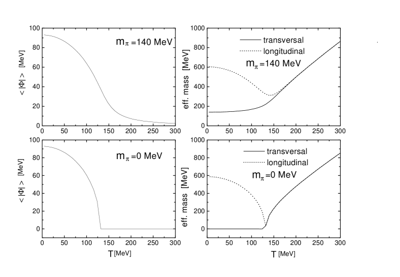
FIG. 2.: The temperature dependence of the magnitude of the order parameter $|\Phi|=\sqrt{\sigma^{2}+\vec{\pi}^{2}}$, the transversal (pion-like) and longitudinal ($\sigma$-like) mass at thermal equilibrium for the physical case of a non-vanishing pion mass and the case without explicit chiral symmetry breaking ($H=0$). The averages are obtained over an ensemble of $10^{3}$ realizations.

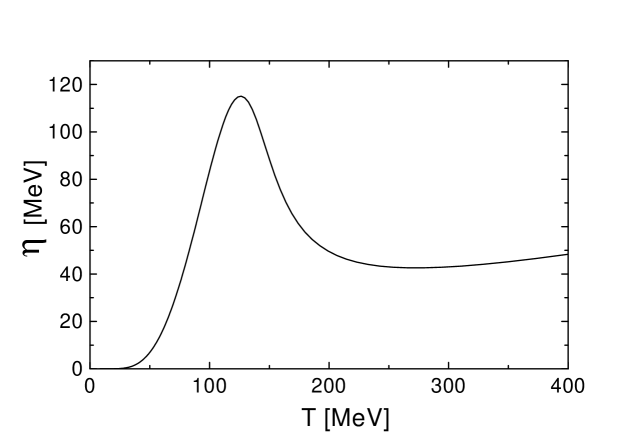
FIG. 3.: The dependence of the friction coefficient $\eta$ on the temperature.

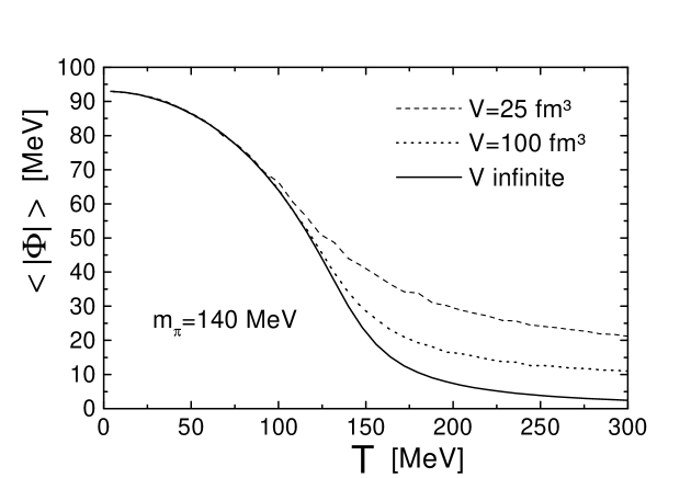
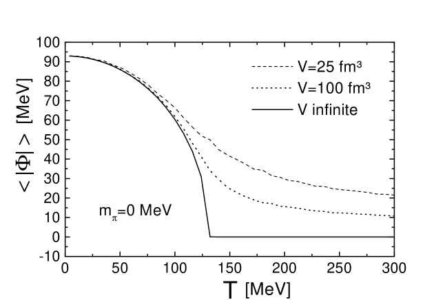
FIG. 4.: The temperature dependence of the magnitude of the order parameter $\Phi$ at thermal equilibrium for different volumes. The averages are obtained over an ensemble of $10^{3}$ realizations.

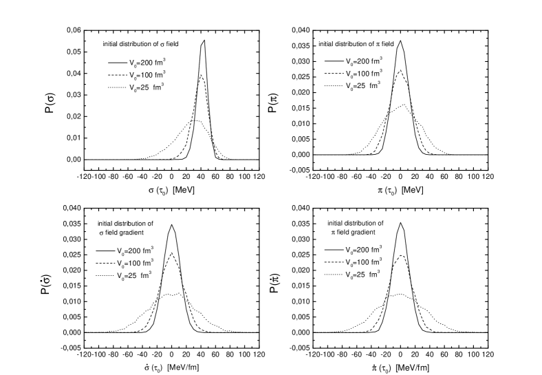
FIG. 5.: Statistical distribution of the chiral $\sigma$ field and one of the three pion fields for different finite volumes. The temperature is taken as the critical temperature $T_{c}$. The distributions are obtained from an ensemble of $10^{4}$ independent realizations.

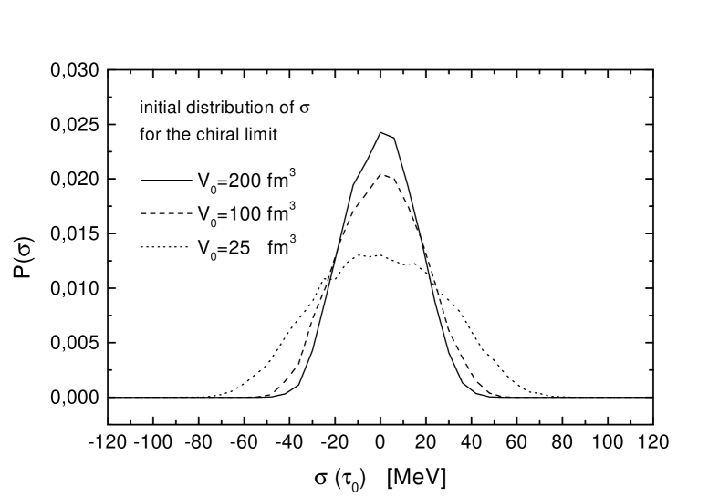
FIG. 6.: Statistical distribution of the chiral $\sigma$ field for different finite volumes for the situation without explicit chiral symmetry breaking. The temperature is taken as the critical temperature $T_{c}$. The distributions are obtained from $10^{4}$ realizations.

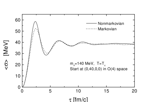
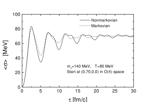
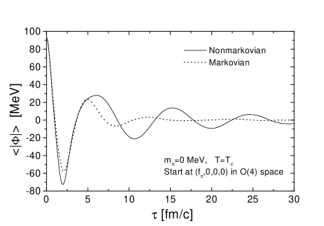
FIG. 7.: Relaxation of the ensemble averaged $\sigma$ field within a heat bath at finite temperature for the nonmarkovian and markovian case. The upper and middle part correspond to the situation of a physical pion mass, whereas the bottom one corresponds to the case without explicit chiral symmetry breaking ($m_{\pi}=0$). In this case we depict the relaxation of the ensemble averaged magnitude of the order parameter. The averages are taken over $10^{3}$ realizations.

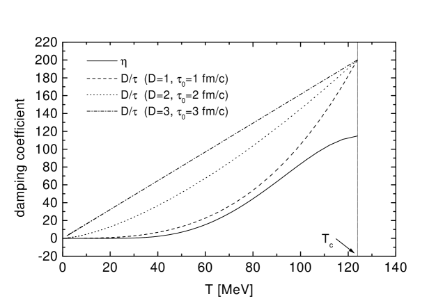
FIG. 8.: Comparison of the friction coefficient $\eta(T)$ with the Raleigh damping term $D/\tau$.

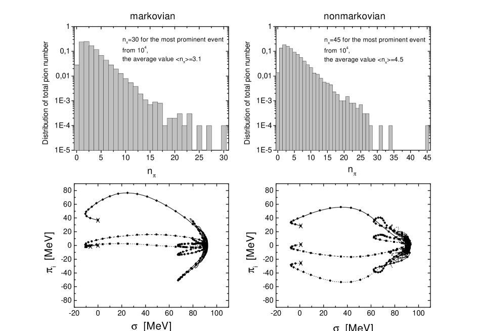
FIG. 9.: Statistical and normalized distribution $P(n_{\pi})$ of the emerging final pion number and the time evolution of the three pionic trajectories ($(\sigma(\tau),\pi_{i}(\tau))$, i=1,2,3,) for the most prominent event within an ensemble of $10^{4}$ realizations in both a markovian and a nonmarkovian simulation. The trajectories start at the initial proper time $\tau_{0}=0.5$ fm/c. The starting points are marked with ‘X’. The marks along the trajectories are positioned at time intervals of $\Delta\tau=0.21$ fm/c.

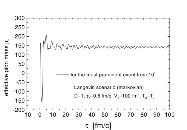
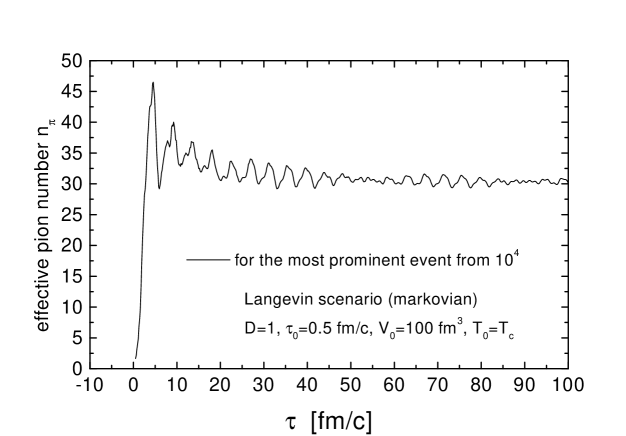
FIG. 10.: The time evolution of the effective pion mass $\mu_{\bot}(\tau)$ and the effective pion number $n_{\pi}(\tau)$ for the most prominent event obtained in the markovian simulation of Fig. 9

.

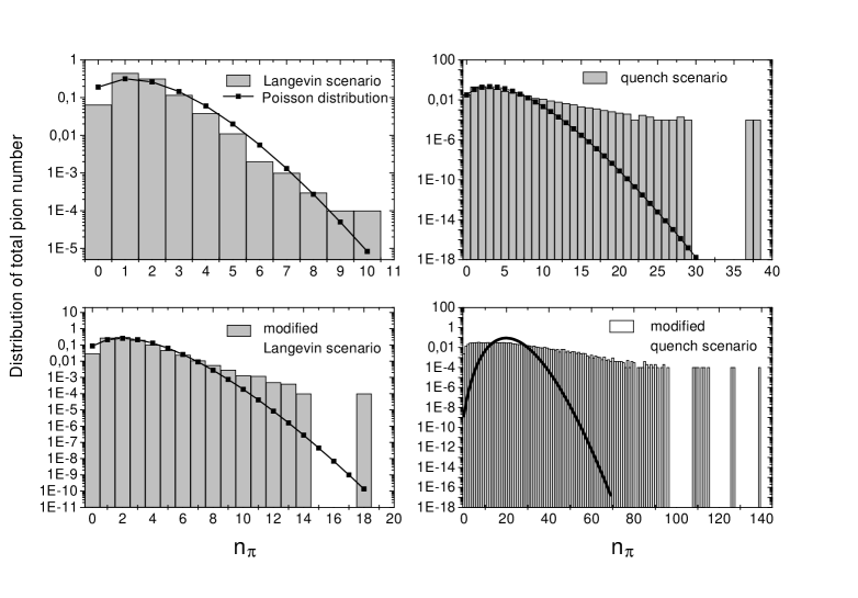
FIG. 11.: Statistical distribution of the final yield in the pion number for four different scenarios (see text) within a (D=)3-dimensional scaling expansion. Each simulation has been performed with $10^{4}$ independent events. The initial volume $V(\tau_{0})=100\,fm^{3}$ and the initial proper time is taken as $\tau_{0}=7\,fm/c$. The distributions are compared with the corresponding Poisson distributions. The averaged pion number in the Langevin, modified Langevin, quench and modified quench scenario are 1.66, 2.45, 3.46 and 20.36 respectively.

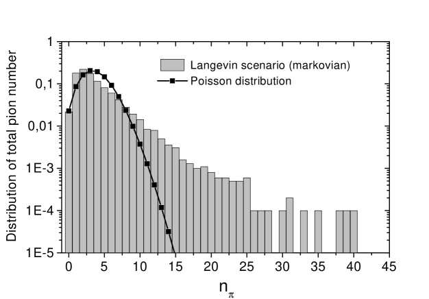
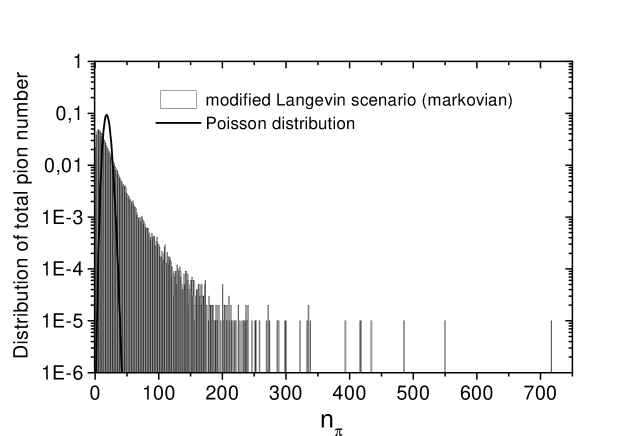
FIG. 12.: Statistical distribution of the final yield in low momentum pion number within the Langevin (upper figure) and modified Langevin (lower figure) scenario compared with the corresponding poissonian distribution. A fast expansion is simulated by choosing $D=3$ and $\tau_{0}=3$ fm/c. The upper distribution is calculated within $10^{4}$ events, whereas for the lower a sample of $10^{5}$ independent events has been chosen.

FIG. 13.: Statistical distribution of the final number of $\sigma$-mesonic excitations within the modified Langevin scenario of Fig. 12 obtained within $10^{4}$ events.

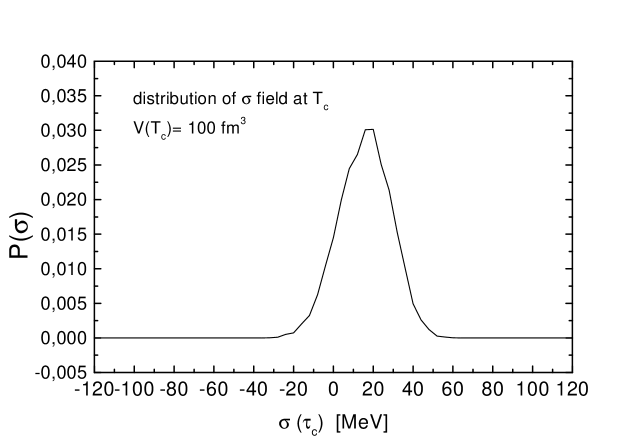
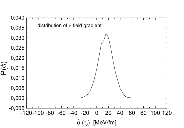
FIG. 14.: Statistical distribution of the $\sigma$ field and its temporal gradient at the time $\tau_{c}=3\,fm/c$ when the critical temperature $T_{c}$ is reached. The time evolution starts at a higher temperature $T_{i}=300$ MeV with a 3-dimensional expansion in the Langevin scenario. The volume at $\tau_{c}$ is 100 $fm^{3}$.

FIG. 15.: The reduced factorial cumulants for $m=1$ to 6 for the pion number distribution obtained within the (markovian) modified Langevin scenario (D=3) for different initial proper times. The initial volume is taken as $V(\tau_{0})=100\,fm^{3}$. The average pion number $\langle\!\langle n_{\pi}\rangle\!\rangle$ within $10^{4}$ events are 54, 18.5, 4.8 and 2.4, respectively, corresponding to $\tau_{0}=$ 2, 3, 5 and 7 fm/c, respectively. In addition the cumulants obtained for a distribution for $\tau_{0}=3$ fm/c within a larger sample of $10^{5}$ events are also shown to estimate the numerical error.

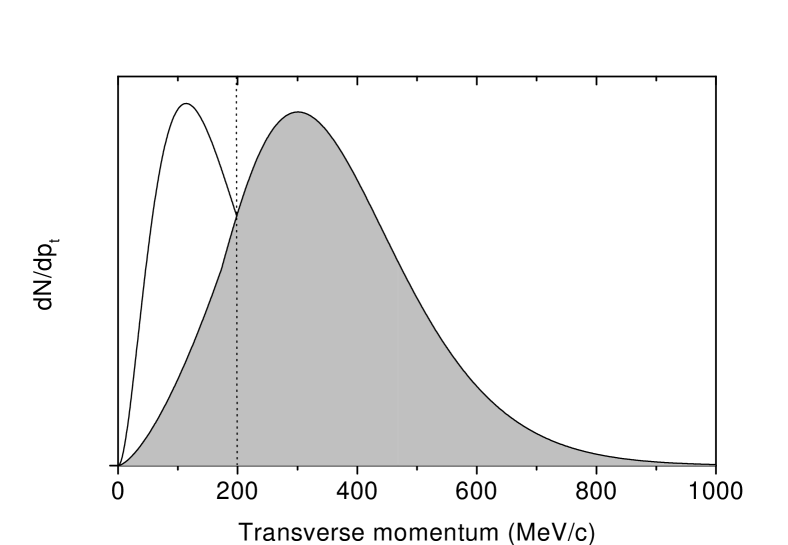
FIG. 16.: Schematic and qualitative view of the transverse momentum spectrum of charged pions for one single event within some definite rapidity interval including a single hypothetical and sufficiently prominent DCC candidate. (This spectrum has been schematically redrawn from a simulated event of background pions to be expected at RHIC energies [43].)

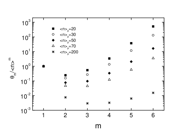
FIG. 17.: The reduced factorial cumulants for $m=1$ to 6 for the pion number distribution of low momentum pions stemming from two independent sources: A distribution stemming from a single emerging DCC taken from the lower part of Fig. 12 (modified Langevin scenario with $D=3$ and $\tau_{0}=3$ fm/c) and a poissonian distributed background pion source with different mean values $\langle n\rangle_{P}=20-200$.

FIG. 18.: Illustration of the solutions and kinematical constraints for $q_{2}$ and $t$ for the three cases (see text). For case I there exists one solution for $q_{2}$ for every $t$. The kinematical constraints $q_{2}^{s_{1}}$ and $q_{2}^{s^{\prime}_{1}}$ are the points where the lines $F(q_{2},1)$ and $F(q_{2},-1)$ cut $\omega_{2}(q_{2})$. For case II there exist two solutions for every $t\in[t_{kr},-1]$. The kinematical constraints $q_{2}^{s_{2}}$ and $q_{2}^{s^{\prime}_{2}}$ are the cut points between $F(q_{2},-1)$ and $\omega_{2}(q_{2})$. For case III all solutions are larger than $q_{2}^{s_{3}}$. It is easy to show that these solutions do not fulfill the equation (A16).

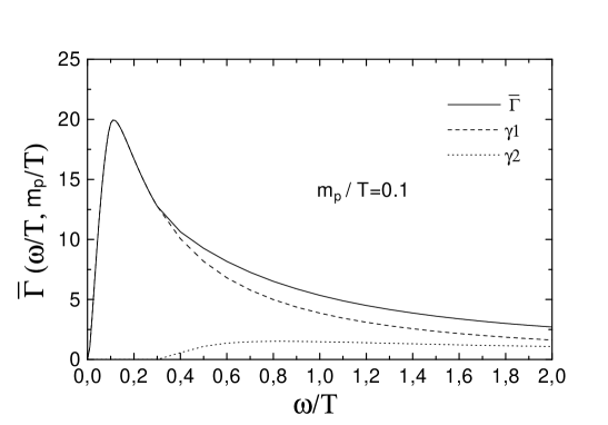
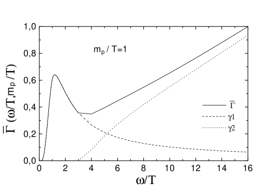
FIG. 19.: The reduced dissipation kernel for $m_{p}/T=0.1$ and $m_{p}/T=1$. $\gamma_{1}$ and $\gamma_{2}$ are the contributions to ${\bar{\Gamma}}$ from the contributing scattering and decay process (see text).

FIG. 20.: The reduced dissipation kernel ($\gamma_{1}$) in time for $T=120$ MeV and a plasmon mass $m_{p}=194$ MeV.

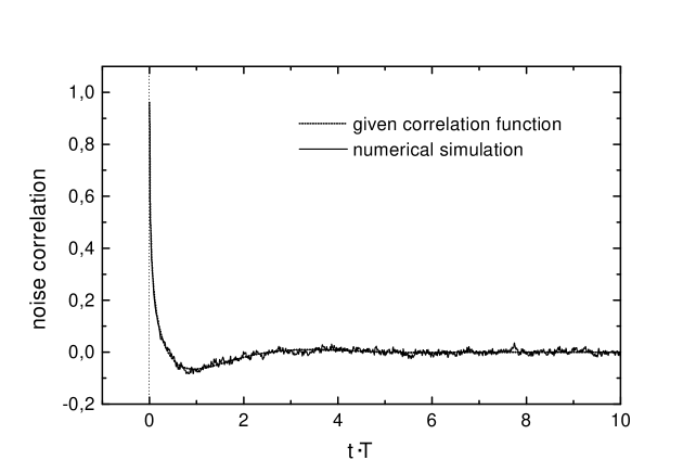
FIG. 21.: Comparsion of the correlation function $I=\langle\!\langle\xi(t)\xi(0)\rangle\!\rangle$ of the numerically generated noise with the given correlation function which is taken as the reduced dissipation kernel of Fig. 20 (lower part). The averaging is performed over an ensemble of $10^{4}$ noise sequences. In addition one exemplaric numerically generated noise sequence dictated by the correlation function is also depicted (upper part).

REFERENCES

- [1] B. Müller, ‘The Physics of the Quark-Gluon Plasma’, Lecture Notes in Physics 225 (1985), Springer, Berlin; ‘Quark-Gluon Plasma’, ed. R. Hwa, Advanced Series on Directions in High Energy Physics, World Scientific, (1990); ‘Quark-Gluon Plasma II’, ed. R. Hwa, Advanced Series on Directions in High Energy Physics, World Scientific, (1995).
- [2] see, e.g., the contribution of C. DeTar in ‘Quark-Gluon Plasma II’ in [1].
- [3] for a review see the contribution of K. Rajagopal in ‘Quark-Gluon Plasma II’ in [1]; and J.-P. Blaizot and A. Krzywicki, Acta Phys. Pol. B 27, 1687 (1996).
- [4] A.A. Anselm, Phys. Lett. B 217, 169 (1989). A.A. Anselm and M.G. Ryskin, Phys. Lett. B 266, 482 (1991).
- [5] D. Bjorken, Int. J. Mod. Phys. A 7, 4819 (1992).
- [6] K. Rajagopal and F. Wilczek, Nucl. Phys. B 404, 577 (1993).
- [7] see, eg, the references listed in [3] for some of the further developments on DCC formation.
- [8] D. Boyanovsky, H.J. de Vega and R. Holman, Phys. Rev. D 51, 734 (1995), F. Cooper, Y. Kluger, E. Mottola and J.P. Paz, Phys. Rev. D 51, 2377 (1995).
- [9] C.M. Lattes, Y. Fujimoto and S. Hasegawa, Phys. Rep. 65, 151 (1980).
- [10] C. Greiner, C. Gong and B. Müller, Phys. Lett. B 316, 226 (1993).
- [11] J. Randrup, Phys. Rev. Lett. 77, 1226 (1996); Nucl. Phys. A 616, 531 (1997).
- [12] M. Asakawa, Z. Huang and X.N. Wang, Phys. Rev. Lett. 74, 3126 (1995).
- [13] S. Gavin and B. Müller, Phys. Lett. B 329, 486 (1994).
- [14] T.S. Biró, D. Molnár, F. Zhongan and L.P. Csernai, Phys. Rev. D 55, 6900 (1997).
- [15] J. Randrup, Phys. Rev. D 55, 1188 (1997).
- [16] T.S. Biró and C. Greiner, Phys. Rev. Lett. 79, 3138 (1997).
- [17] A. K. Chaudhuri, Phys. Rev. D 59, 117503 (1999), hep-ph/9904269; S. Digal, R. Ray, S. Sengupta and A. Srivastava, hep-ph/9805227v2.
- [18] C. Greiner, Z. Xu and T.S. Biro, hep-ph/9809461.
- [19] see, eg, D.U. Jungnickel and C. Wetterich, hep-ph/9902316.
- [20] A. Bochkarev and J. Kapusta, Phys. Rev. D 54, 4066 (1996).
- [21] A. Gocksch, Phys. Rev. Lett. 67, 1701 (1991).
- [22] R. Pisarski and F. Wilczek, Phys. Rev. D 29, 338 (1984); F. Wilczek, Int. J. Mod. Phys. A 7, 3911 (1992).
- [23] C. Greiner and B. Müller, Phys. Rev. D 55, 1026 (1997).
- [24] C. Greiner and S. Leupold, Ann. Phys. 270, 328 (1998).
- [25] R. Feynman and F. Vernon, Ann. Phys. 24, 118 (1963).
- [26] A.O. Caldeira and A.J. Leggett, Physica 121A, 587 (1983).
- [27] P.C. Hohenberg and B.I. Halperin, Rev. Mod. Phys. 49, 435 (1977).
- [28] A. Berera, M. Gleiser and R.O. Ramos, Phys. Rev. D 58, 123508 (1998).
- [29] H. Meyer-Ortmanns and B.-J Schäfer, Phys. Rev. D 53, 6586 (1996).
- [30] J.V. Steele and V. Koch, Phys. Rev. Lett. 81, 4096 (1998).
- [31] M. Pietroni, Phys. Rev. Lett. 81, 2424 (1998), and hep-ph/9809390.
- [32] M. Ishihara and F. Takagi, hep-ph/9908213.
- [33] D.H. Rischke, Phys. Rev. C 58, 2331 (1998).
- [34] L. Csernai, P. Ellis, S. Jeon, J. Kapusta, nucl-th/9908020.
- [35] D. Molnár, L.P. Csernai and Z.I. Lazar, Phys. Rev. D 58, 114018 (1998).
- [36] A. Niegawa, hep-th/9810043.
- [37] J.D. Bjorken, Phys. Rev. D 27, 140 (1983).
- [38] M. Lampert, J. Dawson and F. Cooper, Phys. Rev. D 54, 2213 (1996).
- [39] A. Dumitru, hep-ph/9905217.
- [40] W.H. Press et al., Numerical Recipes, Cambridge University Press (1992).
- [41] J. Borill and M. Gleiser, Phys. Rev. D 51, 4111 (1995); R.M. Haas, Phys. Rev. D 57, 7422 (1998); B. Bergerhoff, M. Lindner and M. Weiser, hep-ph/9909261.
- [42] Z. Xu, C. Greiner and S. Leupold, work in progress.
- [43] R. Bellwied, S. Gavin and T. Humanic, nucl-th/9811085.
- [44] G. Amelino-Camelia, J.D. Bjorken and S.E. Larsson, Phys. Rev. D 56, 6942 (1997).
- [45] A. Krzywicki and J. Serreau, Phys. Lett. B 448, 257 (1999).
- [46] S. Mrowczynski and B. Müller, Phys. Lett. B 363, 1 (1995); H. Hiro-Oka and H. Minakata, hep-ph/9906301.
- [47] H.-T. Elze and I. Sarcevic, Phys. Rev. Lett. 68, 1988 (1992); H.C. Eggers, H.-T. Elze and I. Sarcevic, Int. J. Mod. Phys. A 9, 3821 (1994).
- [48] J. Serreau, private communication.
- [49] R.C. Hwa, Phys. Rev. D 57, 1831 (1998); see also the contribution of R.C. Hwa in ‘Quark-Gluon Plasma II’ in [1].
- [50] M. Aggrarwal et al. (WA98 collaboration), Phys. Lett. B 420, 169 (1998), T.K. Nayak et al. (WA98 collaboration), Nucl. Phys. A 638, 249c (1998); P. Steinberg (WA98 collaboration), Nucl. Phys. B 71, 335 (1999).
- [51] T.C. Brooks et al (MINIMAX collaboration), Phys. Rev. D 55, 5667 (1997).
- [52] Z. Huang, I. Sarcevic, R. Thews, X.-N. Wang, Phys. Rev. D 54, 750 (1996).
- [53] C. Chow and T. Cohen, Phys. Rev. C 60, 05492 (1999).
- [54] A. Bialas and V. Koch, Phys. Lett. B 456, 1 (1999); M. Stephanov, K. Rajagopal and E. Shuryak, hep-ph/9903292; G. Baym and H. Heiselberg, nucl-th/9905022.
- [55] J. Kapusta and A. Vischer, Z. Phys. C 75, 507 (1997); O. Scavenius and A. Dumitru, hep-ph/9905572.
- [56] E. Wang and U. Heinz, Phys. Rev. D 53, 899 (1996).
- [57] R.P. Parwani, Phys. Rev. D 45, 4695 (1992).
- [58] C.V. Heer, ‘Statistical Mechanics, Kinetic Theory, and Stochastic Processes’, Academic Press.
- [59] N.G. van Kampen, ‘Stochastic Processes in Physics and Chemistry’, North-Holland Publ. Comp., Amsterdam (1981).
- [60] A.H. Mueller, Phys. Rev. D 4, 150 (1971).