F. M. Steffens,
Instituto de Física, USP, C. P. 66 318, 05315-970,SP, Brasil

Abstract

We work with two general factorization schemes in order to explore the consequences of imposing scheme independence on $g_{1}^{p}(x,Q^{2})$. We see that although the light quark sector is indifferent to the choice of a particular scheme, the extension of the calculations to the heavy quark sector indicates that a scheme like the $\overline{MS}$ is preferable.

The problem raised by the results of the EMC spin experiment [2] was deeply influential on a substantial part of the 1990’s research in both theoretical and experimental hadron and particle physics. Their data implied that the quark singlet axial charge measured in a proton target, $g_{a}^{0}$, was compatible with zero, while quark model calculations predicted $g_{a}^{0}$ to lie in the range of 0.6 - 0.7. After a series of experiments made at CERN, SLAC and HERA over the past 10 years, it is accepted today that $g_{a}^{0}\approx 0.3$, which is still far from those early theoretical expectations.

In 1974, Ellis and Jaffe proposed a sum rule [3] for the integral in $x$ of $g_{1}^{p}(x)$, where they assumed that the sea quarks in the proton are not polarized. This implies that $\Delta s$, the helicity carried by the strange quarks, is zero. Experimentally, $\int_{0}^{1}g_{1}^{p}(x,Q^{2}=10\;GeV^{2})dx=0.120\pm 0.005\pm 0.006\pm 0.014$ [4], while the Ellis and Jaffe sum rule gives $\int_{0}^{1}g_{1}^{p}(x,Q^{2}=10\;GeV^{2})dx=0.176\pm 0.006$.

In the the parton model, the first moment of $g_{1}^{p}(x)$ is given by $\int_{0}^{1}g_{1}^{p}(x)dx=\frac{1}{12}g_{a}+\frac{1}{36}g_{a}^{8}+\frac{1}{9}g_{a}^{0}$, with $g_{a}=\Delta u-\Delta d$ the isotriplet axial charge, $g_{a}^{8}=\Delta u+\Delta d-2\Delta s$ the octet axial charge, and $g_{a}^{0}=\Delta u+\Delta d+\Delta s$. The parton model structure functions are, actually, QCD structure functions with ${\cal O}(\alpha_{s}^{0})$ corrections. Beyond the parton model, the identification of the singlet axial charges with the sum of the quark helicities ceases to be true, because of the clash between a gauge invariant and a chiral symmetric renormalization procedure of the axial charge [5, 6].

The failure of the Ellis and Jaffe sum rule to agree with the experiments is translated into the non-equivalence between the quark singlet and octet axial charges. From the start there has been a large controversy on the mechanism responsible for $g_{a}^{0}\neq g_{a}^{8}$. In the context of the parton model, $\Delta s\neq 0$ settles the question. However, as proposed by Altarelli and Ross [7], and Carlitz, Collins and Mueller [8], it is still possible to have $\Delta s=0$ if one takes into account the axial anomaly [9] which appears in the QCD calculations of $g_{1}^{p}(x,Q^{2})$ at ${\cal O}(\alpha_{s})$. Later, it became clear that these two different scenarios, $\Delta s\neq 0$ or an anomaly contribution, are simply related by a change of scheme defining the partons distributions and the coefficient functions. This will be, indeed, the main contribution of this work. We will argue that although the appearence of gluons in the first moment of $g_{1}^{p}(x,Q^{2})$, in the light quark sector, is a matter of scheme preference, the introduction of heavy quarks suggests that a scheme where the gluons do not contribute, like the $\overline{MS}$ scheme, is preferable.

A part of what is discussed in this work have already been adressed in the literature. Specifically, the importance in isolating the hard part of the photon-gluon cross section [10, 11, 12, 13]. However, some missconceptions still persist, mainly those connected with the heavy quark contribution to $g_{1}^{p}(x,Q^{2})$, which is one of the motivations for the explicit discussions made here on the ways to calculate a polarized gluon coefficient function which is free of ambiguity in the infrared region.

The choice of a factorization scheme is a reflection of the choice of a regulator and of a subtraction for the soft and collinear divergences appearing in the calculation of the partonic cross sections. In the specific case of the axial anomaly contribution to $g_{1}^{p}$, much have been discussed about the ambiguity in the choice of a quark or of a gluon mass to regulate these divergences [7, 8, 10, 11]. In a satisfactory calculation, the hard part of the partonic cross sections should not present any ambiguity. The infrared singularities are present in the full virtual photon-gluon cross section [14, 15], $\tilde{C}_{g}$, and they appear explicitly when the $Q^{2}\rightarrow\infty$ limit is taken. As a general rule, the divergent (or soft) part of the cross section can be calculated from the expectation value of the quark singlet axial current between off-shell gluon lines [8, 10, 11, 16]:

$$\Delta q^{g}(x,m_{q}^{2},P^{2},\mu^{2}) = -2\alpha_{s}\mu^{-(D-4)}\int\frac{d^{D-2}k_{\perp}}{(2\pi)^{D-2}}\left[\frac{k_{\perp}^{2}(1-2x)-m_{q}^{2}}{(k_{\perp}^{2}+m_{q}^{2}+x(1-x)P^{2})^{2}}\right.$$ (1)

$$\left.-2\frac{D-4}{D-2}(1-x)\frac{k_{\perp}^{2}}{(k_{\perp}^{2}+m_{q}^{2}+x(1-x)P^{2})^{2}}\right],$$

where $P^{2}=-p^{2}$ is the gluon virtuality, $m_{q}$ is the quark mass, and the number of quark flavors was set to 1. For an arbitrary number of flavors, Eq. (1) is multiplyed by $n_{f}$. The integral can be calculated in $D$ dimensions as it stands, and the use of the modified Minimal Subtraction ($\overline{MS}$) method to remove the UV divergence of $\Delta q^{g}$ will define the coefficient functions and parton distributions in that scheme. A second option is to take from the start the limit $D\rightarrow 4$, and use a cutoff $\mu^{2}$ to regularize the mass divergences. This is a momentum subtraction scheme, and the anomalous gluon contribution to the first moment of $g_{1}^{p}(x,Q^{2})$ will appear. Explicitly,

$$\Delta q_{g}^{\overline{MS}}(x,m_{q}^{2},P^{2},\mu^{2})=\frac{\alpha_{s}}{2\pi}\left[(2x-1)ln\left(\frac{\mu^{2}}{m_{q}^{2}+x(1-x)P^{2}}\right)-\frac{m_{q}^{2}}{m_{q}^{2}+x(1-x)P^{2}}+1\right],$$ (2)

$$\Delta q_{g}^{\mu}(x,m_{q}^{2},P^{2},\mu^{2}) = \frac{\alpha_{s}}{2\pi}\left[(2x-1)ln\left(\frac{\mu^{2}+m_{q}^{2}+x(1-x)P^{2}}{m_{q}^{2}+x(1-x)P^{2}}\right)\right.$$ (3)

$$\left.+(1-x)\frac{\mu^{2}}{\mu^{2}+m_{q}^{2}+x(1-x)P^{2}}\frac{2m_{q}^{2}+x(1-2x)P^{2}}{m_{q}^{2}+x(1-x)P^{2}}\right].$$

Both Eqs. (2) and (3) are dependent on the $m_{q}^{2}/P^{2}$ ratio, which is not a real problem because they are only part of the gluon coefficient function. What configures a problem is the attempt to draw conclusions about the possible anomalous gluon contribution to $g_{1}^{p}(x,Q^{2})$ from those two equations. The standard procedure is to look at the subtracted partonic cross sections:

$$C_{g}^{\overline{MS}}(x,Q^{2},\mu^{2}) = \tilde{C}_{g}(x,m_{q}^{2},P^{2},Q^{2})-\Delta q_{g}^{\overline{MS}}(x,m_{q}^{2},P^{2},\mu^{2})$$

$$C_{g}^{\mu}(x,Q^{2},\mu^{2}) = \tilde{C}_{g}(x,m_{q}^{2},P^{2},Q^{2})-\Delta q_{g}^{\mu}(x,m_{q}^{2},P^{2},\mu^{2}).$$ (4)

The hard part of the cross sections should not depend on the $m_{q}^{2}/P^{2}$ ratio for $Q^{2},\mu^{2}>>m_{q}^{2},P^{2}$, which is the reason for the neglect of those two variables in the left hand side of Eq. (4). We also use the label $\overline{MS}$ to denote the fact that the usual $\overline{MS}$ gluon coefficient function is recovered in the large $Q^{2}$ limit. The same for the $C_{g}^{\mu}$ defined in a momentum subtraction scheme.

In the region of low $k_{\perp}$, the integrands of Eq. (1) and of $\tilde{C}_{g}$ are equal. Hence, the fact that the RHS of Eqs. (4) turns out to be nonzero is a reflection of the large $k_{\perp}$ region, and of the UV regulator of Eq. (1): the redefinition of the parton distributions, through an absortion of finite parts of the cross section, is a matter of taste. Depending on the regulator chosen, one can also absorb or not the axial anomaly term into the redefinition of the parton distributions. Explicitly, when $Q^{2},\mu^{2}>>m_{q}^{2},P^{2}$, we have:

$$C_{g}^{\overline{MS}}(x,Q^{2},\mu^{2}) = \frac{\alpha_{s}}{2\pi}\left\{(2x-1)\left[ln\left(\frac{Q^{2}}{\mu^{2}}\right)+ln\left(\frac{1-x}{x}\right)-1\right]+2(1-x)\right\},$$

$$C_{g}^{\mu}(x,Q^{2},\mu^{2}) = \frac{\alpha_{s}}{2\pi}(2x-1)\left[ln\left(\frac{Q^{2}}{\mu^{2}}\right)+ln\left(\frac{1-x}{x}\right)-1\right].$$ (5)

Contrary to repeated claims in the literature [17, 18, 19], the schemes discussed here have a well defined separation of hard effects in the coefficient functions and soft effects in the parton distribuitions. In principle, the polarized light quark sector is well described by both of them. For a better understanding of both schemes, we show in Fig. 1 the integrals in $x$ of Eqs. (5) as a function of $x$, denoted by $I_{0x}=\int_{0}^{x}C_{g}^{\mu,\overline{MS}}(x,Q^{2})dx$. As is well known, $\int_{0}^{1}C_{g}^{\overline{MS}}(x,Q^{2},\mu^{2})=0$, and $\int_{0}^{1}C_{g}^{\mu}(x,Q^{2},\mu^{2})=-1$, in units of $\alpha_{s}/2\pi$. The interesting feature is that the main contribution to both integrals comes from the large $x$ region. In fact, $x=0.001$ is already a good zero, while the $x>0.8$ region is essential to give the integrals the value they have.

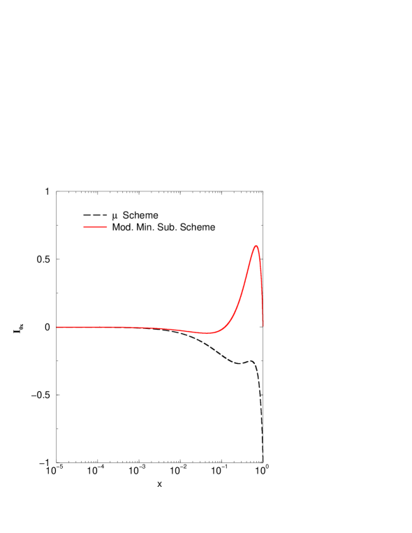
Figure 1: The integral from $0$ to $x$ of the polarized gluon coefficient function as a function of $x$, for the $\overline{MS}$ and $\mu$ schemes, in units of $\alpha_{s}/2\pi$. schemes.

The physical structure function is indifferent to which scheme is used to define the parton distribution and the coefficient functions. This is expressed as:

$$g_{1}^{p}(x,Q^{2}) = \left(\frac{1}{12}g_{a}^{\overline{MS}}(x)+\frac{1}{36}g_{a}^{8,\overline{MS}}(x)\right)\otimes C_{q}^{NS,\overline{MS}}(x,Q^{2})$$ (6)

$$+ \frac{1}{9}g_{a}^{0,\overline{MS}}(x)\otimes C_{q}^{S,\overline{MS}}(x,Q^{2})+\frac{1}{9}\Delta g^{\overline{MS}}(x)\otimes C_{g}^{\overline{MS}}(x,Q^{2})$$

$$= \left(\frac{1}{12}g_{a}^{\mu}(x)+\frac{1}{36}g_{a}^{8,\mu}(x)\right)\otimes C_{q}^{NS,\mu}(x,Q^{2})$$

$$+ \frac{1}{9}g_{a}^{0,\mu}(x)\otimes C_{q}^{S,\mu}(x,Q^{2})+\frac{1}{9}\Delta g^{\mu}(x)\otimes C_{g}^{\mu}(x,Q^{2}).$$

Although we did not write explicitly the $Q^{2}$ dependence of the various distributions, we remind the reader that only the singlet axial charge, in the $\overline{MS}$ scheme, has a $Q^{2}$ dependent first moment.

To ${\cal O}(\alpha_{s})$, $C_{q}(x,Q^{2})\equiv C_{q}^{NS}(x,Q^{2})=C_{q}^{S}(x,Q^{2})=\delta(x-1)+\frac{\alpha_{s}(Q^{2})}{2\pi}C_{q}^{(1)}(x)$. Using Eqs. (5), and the relation between the singlet axial charges between the two schemes, $g_{a}^{0,\overline{MS}}(x,Q^{2})=g_{a}^{0,\mu}(x,Q^{2})-\frac{\alpha_{s}(Q^{2})}{\pi}n_{f}(1-x)\otimes\Delta g(x,Q^{2})$, the second line of Eq. (6) can be rewritten as:

$$g_{1}^{p}(x,Q^{2}) = \left(\frac{1}{12}g_{a}^{\mu}(x)+\frac{1}{36}g_{a}^{8,\mu}(x)\right)\otimes C_{q}^{\mu}(x,Q^{2})$$ (7)

$$+ \frac{1}{9}g_{a}^{0,\overline{MS}}(x)\otimes C_{q}^{\mu}(x,Q^{2})+\frac{1}{9}\Delta g^{\mu}(x)\otimes C_{g}^{\overline{MS}}(x,Q^{2}),$$

where the term $\alpha_{s}^{2}/2\pi^{2}(1-x)\otimes\Delta g(x)\otimes C_{q}^{(1)}(x)$ was disregarded. We can now relate the remaining distributions and coefficient functions in the two schemes in the following way:

$$C_{q}^{\mu}(x) = C_{q}^{\overline{MS}}(x)+\delta C_{q}(x)$$

$$\Delta g^{\mu}(x) = \Delta g^{\overline{MS}}(x)+\delta g(x)$$

$$\frac{1}{12}g_{a}^{\mu}(x)+\frac{1}{36}g_{a}^{8,\mu}(x) = \frac{1}{12}g_{a}^{\overline{MS}}(x)+\frac{1}{36}g_{a}^{8,\overline{MS}}(x)+\delta q(x),$$ (8)

where $\delta C_{q}(x)$, $\delta g(x)$ and $\delta q(x)$ are some general functions, of ${\cal O}(\alpha_{s})$. Their specific form is not of interest to us at this given moment. However, the use of Eqs. (8) in Eq. (7), and the requirement that Eq. (6) is satisfied, produces the following consistency relations:

$$\left(\frac{1}{12}g_{a}^{\overline{MS}}(x)+\frac{1}{36}g_{a}^{8,\overline{MS}}(x)+\frac{1}{9}g_{a}^{0,\overline{MS}}(x)+\delta q(x)\right)\otimes\delta C_{q}(x)$$

$$+\delta q(x)\otimes C_{q}^{\overline{MS}}(x)+\delta g(x)\otimes C_{g}^{\overline{MS}}(x)=0,$$ (9)

$$\left(\frac{1}{12}g_{a}^{\mu}(x)+\frac{1}{36}g_{a}^{8,\mu}(x)+\frac{1}{9}g_{a}^{0,\mu}(x)-\delta q(x)\right)\otimes\delta C_{q}(x)$$

$$+\delta q(x)\otimes C_{q}^{\mu}(x)+\delta g(x)\otimes\left(C_{g}^{\mu}(x)-\frac{\alpha_{s}}{\pi}n_{f}(1-x)\right)=0.$$ (10)

The first moment of Eq. (9) certainly respects the equality, as $\int_{0}^{1}C_{g}^{\overline{MS}}(x)dx=0$ and $\int_{0}^{1}\delta q(x)dx=\int_{0}^{1}\delta C_{q}(x)dx=0$ because of the conservation of the nonsinglet axial current . The conservation of the nonsinglet axial current also imposes, from the first moment of Eq. (10), that $\int_{0}^{1}\delta g(x)dx=0$, because $\int_{0}^{1}C_{g}^{\mu}(x)dx=-n_{f}\alpha_{s}/2\pi\Delta g$. It follows that the first moment of the polarized gluon distribution is the same in the $\overline{MS}$ and $\mu$ schemes, independent of whether $\Delta g$ contributes or not to the first moment of $g_{1}^{p}(x,Q^{2})$, up to the $(\alpha_{s}/2\pi)^{2}\Delta g$ corrections we neglected before. This result is consistent with the fact that $\Delta g$ starts contributing to $g_{1}^{p}(x,Q^{2})$ at ${\cal O}(\alpha_{s})$ only.

Although both schemes are, in principle, equally good to describe $g_{1}^{p}(x,Q^{2})$ in the light quark sector, we should also look at their behavior when heavy quarks are introduced. In particular, we do not want the hard part of the cross sections to depend on $P^{2}$ once the mass of the heavy quark and the factorization scale are fixed. To investigate that, we calculate Eqs. (4) as a function of $P^{2}$ for the charm quark, with $m_{c}=1.5\;GeV$ and $Q^{2}=\mu^{2}=10\;GeV^{2}$. The resulting curves are shown in Fig. 2, normalized by the coefficient functions calculated with $P^{2}=0$. It is clear that $C_{g}^{\overline{MS}}$ is independent of $P^{2}$ in the range $0\leq P^{2}\leq m_{c}^{2}$. The same is not true for $C_{g}^{\mu}$, which shows a strong dependence on $P^{2}$.

Numerically, $\int_{0}^{1}C_{g}^{\overline{MS}}(x,m_{q}^{2}=2.25\;GeV^{2},Q^{2}=10\;GeV^{2})dx\approx 0.4$, in units of $\alpha_{s}(Q^{2})/2\pi$. Of course, this integral changes with $Q^{2}$, going to zero as $Q^{2}\rightarrow\infty$, but it is independent of $P^{2}$ for fixed $Q^{2}$. Hence there is a well defined contribution from gluons to the first moment of $g_{1}^{p}(x,Q^{2})$, in the $\overline{MS}$ scheme, which appears because of the relatively large mass of the charm quark. On the other hand, $\int_{0}^{1}C_{g}^{\mu}(x,m_{q}^{2}=2.25\;GeV^{2},Q^{2}=10\;GeV^{2})dx$ ranges from $\sim-0.18$, at $P^{2}=0$, to $\sim-0.135$, at $P^{2}=m_{c}^{2}$. Although the difference is not numerically significant ($(0.18-0.135)(\alpha_{s}/2\pi)\Delta g\sim 0.001\Delta g$) as long as $\Delta g$ is not very large, the use of the $\mu$ schemes is, to some degree, damaged.

The inclusion of heavy quarks in the framework of perturbative calculation of structure functions have received great attention in the recent literature [20, 21, 22, 23, 24, 25]. These works have focused in the development of shemes that interpolate the pure photon-gluon fussion calculation from the region where $Q^{2}\sim m_{h}^{2}$, to the usual massless approach (when $Q^{2}>>m_{h}^{2}$). A fundamental point of these schemes is that the heavy quark is treated as a massless parton in the Altarelli-Parisi evolution equations, which will have $n_{f}+1$ active flavours, while the quark mass dependence is fully kept in the graphs containing the heavy quark lines in the calculation of the coefficient functions. These schemes are generally refered to as Interpolating Schemes (IS).

The coefficient functions in Eq. (4) incorporate the full mass corrections, and are reduced to the massless case in the limit of large $Q^{2}$. Hence, they are suitable for the calculation of the polarized structure functions for $Q^{2}\sim m_{h}^{2}$ and $Q^{2}>>m_{h}^{2}$, in the spirit of the IS. As in the IS the light and the newly introducded heavy quark distributions should be defined in the same scheme, and as the calculation of the $C_{g}^{\mu}$ for a heavy quark is ambiguous, it follows that, strictly, the $\overline{MS}$ scheme is formally superior to the $\mu$ scheme for the calculation of $g_{1}^{p}(x,Q^{2})$.

As a last remark, we want to stress that the amount of polarized heavy quark in the proton is not given by the integral in $x$ of Eqs. (2) and (3), or from the integral of $\tilde{C}_{g}(x,Q^{2})$ for a given quark mass. From them, one would conclude that $\int_{0}^{1}\Delta q_{g}^{\overline{MS}}(x,m_{q}^{2},P^{2},\mu^{2})dx=0$ for $\mu^{2}=m_{q}^{2}>>P^{2}$, while $\int_{0}^{1}\Delta q_{g}^{\mu}(x,m_{q}^{2},P^{2},\mu^{2})dx=\alpha_{s}/4\pi$ in that same limit. In a framework where heavy quark mass effects are systematically included, one should introduce a polarized heavy quark distribution in the proton ($\Delta h(x,Q^{2})$) at the factorization scale $\mu^{2}$, with $\Delta h(x,\mu^{2})=0$. As we saw here, both $\overline{MS}$ and $\mu$ schemes are suitable for this purpose once Eqs. (4) are given, although, in principle, the $\overline{MS}$ scheme has the technical advantage of having a $P^{2}$ independent gluon coefficient function in the heavy quark sector.
I would like to thank X. Ji and A. W. Thomas for valuable discussions. This work was supported by FAPESP (under contracts 96/7756-6 and 98/2249-4).

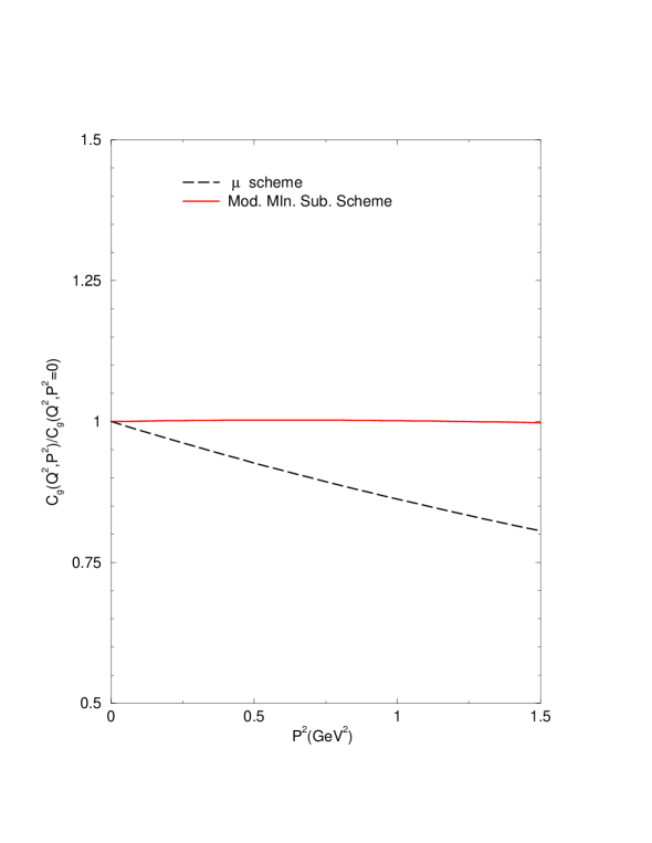
Figure 2: The integrated (in $x$) polarized gluon coefficient function in the $\overline{MS}$ and $\mu$ schemes, as a function of $P^{2}$.

References

[1]
[2] EMC Collaboration, J. Ashman et al., Phys. Lett. B 206
(1988) 364; Nucl. Phys. B328 (1989) 1.
[3] J. Ellis and R. L. Jaffe, Phys. Rev. D9 (1974) 1444.
[4] SMC Collaboration, B. Adeva et al.,
Phys. Rev. D 58 (1998) 112002.
[5] W. Bardeen, Nucl. Phys. B 75 (1974) 246;
R. J. Crewther, Acta Physica Austriaca Suppl. XIX (1978) 47.
[6] G. Veneziano,
Mod. Phys. Lett. A4 (1989) 1605;
S. D. Bass, R. J. Crewther, F. M. Steffens and A. W. Thomas,
hep-ph/9701213.
[7] G. Altarelli and G. G. Ross,
Phys. Lett. B212 (1988) 391.
[8] R. D. Carlitz, J. C. Collins and A. H. Mueller,
Phys. Lett. B214 (1988) 229.
[9] S. L. Adler, Phys. Rev. 177 (1969) 2426;
J. S. Bell and R. Jackiw, Nuovo Cim. 60 (1969) 47.
[10] G. T. Bodwin and J. Qui,
Phys. Rev. D41 (1990) 2756.
[11] L. Mankiewicz,
Phys. Rev. D43 (1991) 64.
[12] F. M. Steffens and A. W. Thomas,
Phys. Rev. D 53 (1996) 1191.
[13] Hai-Yang Cheng,
Int. J. Mod. Phys. A11 (1996) 5109.
[14] S. D. Bass, N. N. Nikolaev and A. W. Thomas,
Report No. ADP-133-T-80, 1990 (unpublished)
[15] W. Vogelsang,
Z. Phys. C50 (1991) 275.
[16] G. P. Lepage and S. J. Brodsky,
Phys. Rev. D22 (1980) 2157.
[17] R. D. Ball, S. Forte and G. Ridolfi,
Phys. Lett. B378 (1996) 255.
[18] E. Leader, A. V. Sidorov and D. B. Stamenov,
Phys. Lett. B445 (1998) 232.
[19] E. Leader,
J. Phys. G 25 (1999) 1557.
[20]
M.A.G. Aivazis, J.C. Collins, F.I. Olness and W.-K. Tung,
Phys. Rev. D 50 (1994) 3102.
[21]