Abstract

A nonrelativistic boundstate formalism used in contemporary calculations is investigated. It is known that the effective Hamiltonian of the boundstate system depends on the choice of gauge. We obtain the transformation charge $Q$ of the Hamiltonian for an arbitrary infinitesimal change of gauge, by which gauge independence of the mass spectrum and gauge dependences of the boundstate wave functions are dictated. We give formal arguments based on the BRST symmetry supplemented by power countings of Coulomb singularities of diagrams. For illustration: (1)we calculate $Q$ up to ${\cal O}(1/c)$, (2)we examine gauge dependences of diagrams for a decay of a $q\bar{q}$ boundstate up to ${\cal O}(1/c)$ and show that cumbersome gauge cancellations can be circumvented by directly calculating $Q$. As an application we point out that the present calculations of top quark momentum distribution in the $t\bar{t}$ threshold region are gauge dependent. We also show possibilities for incorrect calculations of physical quantities of boundstates when the on-shell matching procedure is employed. We give a proof of a justification for the use of the equation of motion to simplify the form of a local NRQCD Lagrangian. The formalism developed in this work will provide useful cross checks in computations involving NRQED/NRQCD boundstates.

1 Introduction

Recently there has been much progress in our theoretical understanding of nonrelativistic QED and QCD (NRQED and NRQCD) boundstates such as positronium, $\Upsilon$ and remnant of toponium boundstates. Following the idea of nonrelativistic effective field theory proposed by Caswell and Lepage [1], formalisms necessary for precise descriptions of these boundstates have been developed significantly [2]-[11]. At the same time there appeared many new calculations of higher order corrections to physical quantities of both the NRQED [12]-[14] and NRQCD boundstates [15]-[24] (boundstate mass, decay width, production and decay cross sections, etc.). Despite these developments, a completely systematic formulation necessary for computations of these physical quantities in perturbative expansions has not been established yet. Among current best technologies the asymptotic expansion of Feynman diagrams [8] seems to be most suited for calculations of the physical quantities, in particular for fixed-order calculations. In addition, effective field theories are powerful tools in order to sum up various large logarithms originating from the widely separated scales inherent in the problems. Efficiencies and correctness of various effective theories are, however, still under debate. (See Refs. [8, 10] for discussions on the current status of the formalisms.)

A notable characteristic in these new developments is that the conventional Bethe-Salpeter equation is no longer being used to calculate the spectrum and wave functions of boundstates. Instead, one starts from the non-relativistic Schrödinger equation (of quantum mechanics) with the Coulomb potential. Then one adds to the nonrelativistic Hamiltonian relativistic corrections and radiative corrections as perturbations to obtain an effective Hamiltonian (quantum mechanical operator) valid up to a necessary order of perturbative expansion. Effective Hamiltonians used in these new formalisms are known to be dependent on the choice of gauge.

The purpose of this paper is to investigate gauge dependence of a nonrelativistic boundstate formalism used in contemporary calculations [3],[14],[16]-[20],[23], which is also closely tied to the potential-NRQCD formalism [7]. Our motivations for the study are: (I) In the present frontier calculations of higher order corrections to physical quantities of boundstates, often the Feynman gauge is used to calculate typically ultraviolet radiative corrections whereas the Coulomb gauge is used to calculate corrections originating typically from infrared regions. Although much care has been taken to calculate consistently in each gauge separately gauge independent subsets of the corrections, it is desirable to clarify gauge dependences of the formalisms actually used in these calculations. (II) We would like to find transformations of boundstate wave functions when we change the gauge-fixing condition. We may apply these transformations to study various amplitudes involving boundstates. Since a physical amplitude is gauge independent, once we know how the wave function transforms, we know how other parts of the amplitude should transform to cancel gauge dependence as a whole. This would provide a useful cross check for identifying all the contributions that have to be taken into account at a given order of perturbative expansion.

Already some time ago, gauge independence of the mass spectrum of the NRQED boundstates was shown and studied in detail based on the Bethe-Salpeter formalism [25]-[27]: Ref. [25] gave a brief discussion; Ref. [26] examined a Feynman gauge calculation of the boundstate spectrum at next-to-leading order very closely and showed that an infinite number of two-particle irreducible diagrams contribute in this gauge, which in the end all cancel due to fairly complicated gauge cancellations (This feature is much more complicated in comparison to the calculation in Coulomb gauge.); Refs. [27] gave formal arguments as well as perturbative analyses which apply to all orders of perturbation series.

In comparison to these earlier works, new achievements of the present work are:

• We use the BRST symmetry to formulate our arguments, which allows us to treat both the NRQED and NRQCD boundstates on an equal footing. In particular we are able to discuss gauge dependence of the NRQCD boundstate formalism rigorously using this symmetry.

• Presently, there exist several different definitions of an effective Hamiltonian beyond leading order. We introduce an effective Hamiltonian defined naturally in the context of time-ordered (or “old-fashioned”) perturbation theory of QED/QCD. Then we obtain a transformation charge $Q$ (quantum mechanical operator) such that the effective Hamiltonian and the boundstate wave function change as

  $$\delta H_{\rm eff}(P^{0})=\left[H_{\rm eff}(P^{0})-P^{0}\right]\,iQ(P^{0})-iQ^{\dagger}(P^{0})\,\left[H_{\rm eff}(P^{0})-P^{0}\right],$$

  $$\delta\varphi=-i\,Q\cdot\varphi$$

  when the gauge-fixing condition is varied infinitesimally. Also, gauge independence of the spectrum is shown using the transformation. We define the charge $Q$ of the effective Hamiltonian directly in terms of the BRST charge and the field operators in the QED/QCD Lagrangian.

• For illustration: (1)we calculate the transformation charge $Q$ at next-to-leading order; (2)we demonstrate gauge cancellations among diagrams by examining an infinitesimal gauge transformation of the amplitude for a $q\bar{q}$ boundstate decaying into $q^{\prime}\bar{q}^{\prime\prime}W^{+}W^{-}$. From the latter example, one can deduce that the present calculations of the top momentum distribution in the $t\bar{t}$ threshold region at next-to-next-to-leading order are gauge dependent.

Another subject of this paper is to study the problems in a determination of the effective Hamiltonian from the on-shell scattering amplitude of a fermion and an antifermion. Generally a fermion and an antifermion inside a boundstate are off-shell so that use of a Hamiltonian determined in the on-shell matching procedure may lead to incorrect calculations of the physical quantities of the boundstate. We clarify this point.

The same problems do not occur if we use a local NRQED/NRQCD Lagrangian and determine (Wilson) coefficients in the Lagrangian by matching onto the full theory, i.e. by matching on-shell amplitudes of all relevant physical processes to those of perturbative QED/QCD in nonrelativistic regions. In this case one should calculate amplitudes for a number of processes to determine all the coefficients. The problems are also related to the use of the equation of motion to simplify the Lagrangian since the on-shell condition is the equation of motion for an asymptotic field. For comprehensiveness we prove in an appendix that it is justified to use the equation of motion to simplify the local NRQED/NRQCD Lagrangian and also to simplify local current operators; to the best of our knowledge such a proof has never been provided explicitly, although similar proofs for other effective field theories have been given [28, 29] and the claim itself is widely accepted already.

Below we will use the language of QCD consistently; nevertheless all of our arguments hold also for the QED boundstates. Throughout the paper we neglect non-perturbative effects (those effects which are typically parametrized by $\Lambda_{\rm QCD}$) and restrict ourselves to arguments which can be understood from a summation of perturbation series in $\alpha_{S}$ to all orders.

The organization of this paper is as follow. After reviewing general aspects of gauge dependence of the conventional relativistic $q\bar{q}$ boundstate formalism (Sec. 2), we summarize characteristic properties of the nonrelativistic boundstates from the viewpoint of the leading Coulomb singularities: their gauge independence and some nontrivial features are explained (Sec. 3). Then we define the effective Hamiltonian $H_{\rm eff}$ for a $q\bar{q}$ system and investigate its gauge dependence as well as gauge dependences of the spectrum and wave functions of the boundstates using the BRST symmetry, within the framework of perturbative expansions in $1/c$; in particular we define the transformation charge $Q$ of the effective Hamiltonian (Sec. 4, App. C). We clarify possible problems in the determination of $H_{\rm eff}$ if one uses the on-shell matching procedure (Sec. 5). For illustration, we present a calculation of the charge $Q$ at ${\cal O}(1/c)$, corresponding to an infinitesimal gauge transformation from the Coulomb gauge; we also examine gauge cancellations in the decay amplitude of a $q\bar{q}$ boundstate into $q^{\prime}\bar{q}^{\prime\prime}W^{+}W^{-}$ at the same order (Sec. 6). Conclusion and discussion are given in Sec. 7. In App. A we give a proof to justify the use of the equation of motion to simplify a local NRQCD Lagrangian. Some detailed discussions are given in App. B and C.

2 Gauge Dependence of the Relativistic Boundstate Formalism: General Aspects

We consider the BRST invariant QCD Lagrangian

$${\cal L}=-\frac{1}{2}\,{\rm tr}\left[G^{\mu\nu}G_{\mu\nu}\right]+\sum_{f}\bar{\psi}_{f}[i\!\not\!\!D(A)-m_{f}]\,\psi_{f}+{\cal L}_{\rm GF+FP},$$ (1)

where generally the sum of gauge-fixing and ghost terms can be written in a BRST exact form as

$${\cal L}_{\rm GF+FP}=\left\{iQ_{B},{\rm tr}[\bar{c}F]\right\}$$ (2)

with the BRST charge $Q_{B}$ and an arbitrary gauge-fixing function $F=F(A,\psi,\bar{\psi},c,\bar{c},B)$ [30].

Define a four-point function (Fig. 1) as

$$G(x_{1},x_{2},x_{3},x_{4}) = \left<{0}\,\right|T\,\psi(x_{1})\overline{\psi}(x_{2})\overline{\psi}(x_{3})\psi(x_{4})\left|\,{0}\,\right>$$ (4)

$$= \int{\textstyle\frac{d^{4}p}{(2\pi)^{4}}\frac{d^{4}q}{(2\pi)^{4}}\frac{d^{4}P}{(2\pi)^{4}}}\,G(p\,qP)$$

$$\times\exp\biggl{[}-i{\textstyle\frac{P}{2}\cdot(x_{1}+x_{2}-x_{3}-x_{4})-ip\cdot(x_{1}-x_{2})+iq\cdot(x_{3}-x_{4})}\biggr{]}.$$

Here and hereafter we restrict our discussions to a quark/antiquark of some specific flavor and omit the flavor index $f$. The field operators and states are those of the Heisenberg picture.

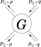
Figure 1: The four-point function $G(pqP)$. $P/2\pm q$ denotes the four-momentum of incoming quark/antiquark; $P/2\pm p$ denotes the four-momentum of outgoing quark/antiquark.

A quark-antiquark boundstate contributes a pole to the Green function $G(p\,qP)$. In the vicinity of a pole corresponding to a boundstate $\left|\,{\nu;\vec{P}}\,\right>$ (with quantum number $\nu$, mass $M_{\nu}$ and momentum $\vec{P}$), the Green function takes a form [31]

$$G(p\,qP)=\frac{i}{2\omega_{\nu,\vec{P}}}\,\frac{\chi_{\nu,\vec{P}}(p)\overline{\chi}_{\nu,\vec{P}}(q)}{P^{0}-\omega_{\nu,\vec{P}}+i\epsilon}\,+(\mbox{regular as }P^{0}\rightarrow\omega_{\nu,\vec{P}}),$$ (5)

where

$$\left<{0}\,\right|T\,\psi(x_{1})\overline{\psi}(x_{2})\left|\,{\nu;\vec{P}}\,\right>=e^{-i(\omega_{\nu,\vec{P}}X^{0}-\vec{P}\cdot\vec{X})}\int{\textstyle\frac{d^{4}p}{(2\pi)^{4}}}\,e^{-ip\cdot x}\,\chi_{\nu,\vec{P}}(p),$$ (6)

$$\overline{\chi}_{\nu,\vec{P}}(p)=\chi_{\nu,\vec{P}}(p)^{\dagger}(\gamma^{0}\otimes\gamma^{0}),$$ (7)

$${\textstyle X=\frac{1}{2}(x_{1}+x_{2}),~{}~{}~{}x=x_{1}-x_{2}},~{}~{}~{}\omega_{\nu,\vec{P}}=\sqrt{\vec{P}^{2}+M_{\nu}^{2}}.$$ (8)

In this paper we assume that the decay width of a boundstate is infinitesimally small except where it is stated otherwise.

An infinitesimal deformation of the gauge-fixing function, $F\rightarrow F+\delta F$, induces a change of the Lagrangian

$$\int d^{4}x\,\delta{\cal L}=\{iQ_{B},\delta{\cal O}\},~{}~{}~{}~{}~{}~{}~{}~{}~{}~{}\delta{\cal O}\equiv\int d^{4}x\,{\rm tr}[\bar{c}\,\delta F].$$ (9)

Accordingly the Green function changes as

$$\delta G(x_{1},x_{2},x_{3},x_{4}) = -\left<{0}\,\right|T\,\{Q_{B},\delta{\cal O}\}\,\psi(x_{1})\overline{\psi}(x_{2})\overline{\psi}(x_{3})\psi(x_{4})\left|\,{0}\,\right>$$ (10)

$$= -\left<{0}\,\right|T\,\delta{\cal O}\,[Q_{B},\psi(x_{1})\overline{\psi}(x_{2})\overline{\psi}(x_{3})\psi(x_{4})]\left|\,{0}\,\right>.$$ (11)

Suppose we are interested in the boundstates which can be created from the vacuum via gauge invariant operators, e.g. $\overline{\psi}(x)\psi(x),~{}\overline{\psi}(x)\!\not{\!\!D}\psi(x),~{}\overline{\psi}(x)\gamma^{\mu}\psi(x)$, etc. For example, in the above Green function we may set $x_{1}=x_{2}\equiv x$, $x_{3}=x_{4}\equiv y$ and contract color indices to make color singlet operators $\overline{\psi}(x)\psi(x)$, $\overline{\psi}(y)\psi(y)$. It then follows from $[Q_{B},\overline{\psi}\psi]=0$ that

$$\delta G(x,x,y,y)\biggr{|}_{\mbox{\scriptsize color singlet}}=0.$$ (12)

Comparing this with eq. (5), one sees that both the mass and the residue of any boundstate which couples to the operator $\overline{\psi}\psi$ are invariant:

$$\delta M_{\nu}=0$$ (13)

and

$$\delta\left<{0}\,\right|\,\overline{\psi}(x)\psi(x)\left|\,{\nu;\vec{P}}\,\right>=0,~{}~{}~{}~{}~{}~{}~{}~{}~{}~{}\mbox{i.e.}~{}~{}\delta\int{\textstyle\frac{d^{4}p}{(2\pi)^{4}}}\,\chi_{\nu,\vec{P}}(p)\biggr{|}_{\mbox{\scriptsize color singlet}}=0.$$ (14)

Since both $\left|\,{0}\,\right>$ and $\overline{\psi}(x)\psi(x)$ are BRST invariant, it implies that the boundstate satisfies the physical state condition

$$Q_{B}\left|\,{\nu;\vec{P}}\,\right>=0.$$ (15)

Note, however, that generally the boundstate wave function $\chi_{\nu,\vec{P}}(p)$ depends on the gauge-fixing condition:

$$\delta\chi_{\nu,\vec{P}}(p) = -\,\mbox{F.T.}\,\left<{0}\,\right|T\,\delta{\cal O}\,[Q_{B},\psi(x)\overline{\psi}(y)]\left|\,{\nu;\vec{P}}\,\right>$$ (16)

$$= -\,\mbox{F.T.}\,\left<{0}\,\right|T\,g\,\delta{\cal O}\,[c(x)\psi(x)\overline{\psi}(y)+\psi(x)\overline{\psi}(y)c(y)]\left|\,{\nu;\vec{P}}\,\right>,$$

where F.T. stands for an appropriate Fourier transform.

Any physical amplitude $\left<{f;{\rm out}}\,\vrule\,{i;{\rm in}}\right>$ which involves the quark-antiquark boundstate contributions includes the above Green function $G(pqP)$ as a part of it. Since the initial and final states satisfy the physical state conditions $Q_{B}\left|\,{i;{\rm in}}\,\right>=Q_{B}\left|\,{f;{\rm in}}\,\right>=0$ and the theory is BRST invariant, the amplitude is gauge independent. Hence, the boundstate poles included in the amplitude are also gauge independent. An interesting question is whether the Green function $G(pqP)$ includes any unphysical pole, which does not contribute to the physical amplitude, close to or degenerate with one of the physical boundstate poles. As for nonrelativistic quark-antiquark boundstates the answer is no, as will be shown in Section 4 and in Appendix C.

3 Nonrelativistic Boundstates: Leading Coulomb Singularities

It is well-known that, in describing a system of a nonrelativistic color-singlet quark-antiquark ($q\bar{q}$) pair, naive perturbation theory breaks down due to formation of boundstates [32, 33]. Intuitively, this is because the slow $q$ and $\bar{q}$ are trapped by the attractive force mediated by exchange of gluons and multiple exchange of gluons between the pair becomes significant. We review this property in a production process of a $q\bar{q}$ pair.

Consider the amplitude of a virtual photon decaying into $q$ and $\bar{q}$, $\gamma^{*}\rightarrow q\bar{q}$, just above the threshold. As we will see below, the ladder diagram for this process with $n$ gluon exchanges has a behavior $\sim(\alpha_{S}/\beta)^{n}$, see Fig. 2.

Figure 2: The ladder diagrams for the process $\gamma^{*}\rightarrow q\bar{q}$. The diagram where $n$ uncrossed gluons are exchanged has a behavior $\sim(\alpha_{S}/\beta)^{n}$ near threshold.

Here, $\beta$ is the velocity of $q$ or $\bar{q}$ in the c.m. frame,

$$\beta=\sqrt{1-\frac{4m^{2}}{s}}.$$ (17)

Hence, the contribution of the $n$-th ladder diagram will not be small even for a large $n$ if $\beta\hbox{ \raise 3.0pt\hbox to0.0pt{$<$}\raise-3.0pt\hbox{$\sim$} }\alpha_{S}$. That is, higher order terms in $\alpha_{S}$ remain unsuppressed in the threshold region. These singularities in $\beta$ which appear in this specific kinematical configuration is known as the “Coulomb singularities” or “threshold singularities”. The singularities arise because, for a particular assignment of the loop momenta, all the internal particles can simultaneously become almost on-shell as $\beta\rightarrow 0$.

The appearance of the factor $(\alpha_{S}/\beta)^{n}$ may be seen as follows. First, consider the one-loop diagram. Its imaginary part can be estimated using the Cutkosky rule (cut-diagram method), see Fig. 3.

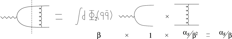
Figure 3: The Cutkosky rule for evaluating the imaginary part of the 1-loop diagram. The factors in $\alpha_{S}$ and $\beta$ are shown explicitly.

Namely, the imaginary part is given by the phase space integration of the product of tree diagrams. The intermediate $q\bar{q}$ phase space is proportional to $\beta$ as

$$d\Phi_{2}(q\bar{q})=\frac{\beta}{16\pi}\,d\cos\theta,$$ (18)

where $\theta$ is the angle between the momenta of the intermediate and final quarks in the c.m. frame. The $q\bar{q}$ scattering diagram with a $t$-channel gluon exchange contributes a factor $\sim\alpha_{S}/\beta^{2}$ since the gluon propagator is proportional to $1/\beta^{2}$; the propagator denominator is given by

$$k^{2}=-|\vec{k}|^{2}=-\,\frac{s\beta^{2}}{2}(1-\cos\theta),$$ (19)

where $k$ denotes the gluon momentum. Thus, we see that the imaginary part of the one-loop diagram has the behavior $\sim\beta\cdot\alpha_{S}/\beta^{2}=\alpha_{S}/\beta$. Analyticity implies that the real part of the one-loop diagram has the same structure $\sim\alpha_{S}/\beta$. By repeatedly using the cut-diagram method, one can show by induction that the imaginary part of the ladder diagram with $n$ uncrossed gluons behaves as $\sim(\alpha_{S}/\beta)^{n}$, see Fig. 4.

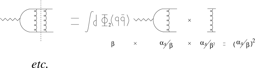
Figure 4: The cut-diagram method for evaluating the singularities of the higher order ladder diagrams. The factors in $\alpha_{S}$ and $\beta$ are shown explicitly.

Alternatively this fact can be shown by a power counting method [8]. The relevant loop momenta in the loop integrals are in the nonrelativistic regime:

$$p^{0}-m,\,\bar{p}^{0}-m\sim{\cal O}(\beta^{2}), ~{}~{}\vec{p}=-\vec{\bar{p}}\sim{\cal O}(\beta),$$

$$k^{0}\sim{\cal O}(\beta^{2}),~{}~{} \vec{k}\sim{\cal O}(\beta).$$ (20)

Here, $p$, $\bar{p}$ and $k$ represent the internal momenta of $q$, $\bar{q}$ and the gluon, respectively, in the c.m. frame. For such configurations, $q(\bar{q})$ and gluon propagators are counted as $\sim 1/\beta^{2}$, and the measure for each loop integration $d^{4}k/(2\pi)^{4}$ as $\sim\beta^{5}$.

Thus, the ladder diagrams contain the leading singularities $\sim(\alpha_{S}/\beta)^{n}$. Other diagrams (in particular crossed gluon diagrams) do not possess the leading singularities but only non-leading singularities $\sim\alpha_{S}^{n+l}/\beta^{n}~{}$ ($l\geq 1$).

As the higher order terms in $\alpha_{S}$ cannot be neglected near threshold, we are led to sum up the leading Coulomb singularities. Let us first discuss gauge dependence of the amplitude when this summation is performed, in particular because only the ladder diagrams are included. The exact amplitude for the process $e^{+}e^{-}\rightarrow q\bar{q}$ near threshold can be expanded in terms of $\alpha_{S}$ and $\beta$ as

$${\cal M}^{(full)}(\alpha_{S},\beta)=\sum_{n=0}^{\infty}\,c_{n}(\alpha_{S}/\beta)^{n}\,+\,(\mbox{non-leading terms}).$$ (21)

The full amplitude ${\cal M}^{(full)}$ is gauge independent, so must be the each coefficient $c_{n}$. Because only the ladder diagrams possess this type of singularities, the most singular part of the ladder diagrams has to be gauge independent.

To see this explicitly, we examine gauge dependence of the gluon propagator. In a general covariant gauge, the $q\bar{q}\rightarrow q\bar{q}$ scattering amplitude in the threshold region is given by

$$\bar{u}_{f}\gamma^{\mu}u_{i}\,\,\frac{-i}{k^{2}+i\epsilon}\left[g_{\mu\nu}-(1\!-\!\xi)\frac{k_{\mu}k_{\nu}}{k^{2}}\right]\bar{v}_{i}\gamma^{\nu}v_{f}=\bar{u}_{f}\gamma^{0}u_{i}\,\,\frac{-i}{-\vec{k}^{2}+i\epsilon}\,\,\bar{v}_{i}\gamma^{0}v_{f}~{}\times~{}\biggl{[}1+{\cal O}(\beta)\biggr{]},$$

(22)

where the subscripts $i$ and $f$ stand for the initial and final state, respectively. We have used the fact that the space components of the currents, $\bar{u}_{f}\gamma^{\mu}u_{i}$ and $\bar{v}_{i}\gamma^{\nu}v_{f}$, are order $\beta$ in the c.m. frame. Note that the leading part of the gluon propagator is identical with the Coulomb propagator in the Coulomb gauge. Eq. (22) also holds for the momenta (20) if we note that the off-shell $q$ and $\bar{q}$ wave functions are given by

$$\not\!p+m=m(1+\gamma^{0})+{\cal O}(\beta),$$ (23)

$$-\!\not\!\bar{p}+m=m(1-\gamma^{0})+{\cal O}(\beta).$$ (24)

Thus, gauge independence of $c_{n}$’s is ensured by gauge independence of the leading part $\sim 1/\beta^{2}$ of the gluon propagator in eq. (22).

Let us denote by $\Gamma^{\mu}$ the sum of the leading singularities of the vertex $\gamma^{*}\rightarrow q\bar{q}$. It satisfies a self-consistent equation as depicted in Fig. 5.

Figure 5: The self-consistent equation satisfied by the leading singularities of the $q\bar{q}\gamma$ vertex $\Gamma^{\mu}$. One should take only the leading part $\sim(\alpha_{S}/\beta)^{n}$ on both sides of the equation.

Retaining only the leading part $\sim(\alpha_{S}/\beta)^{n}$ on both sides of the equation, one obtains the vertex $\Gamma^{\mu}$ as

$$\Gamma^{\mu}=-\,\left(\frac{1+\gamma^{0}}{2}\gamma^{\mu}\frac{1-\gamma^{0}}{2}\right)\,(E-\vec{p}\,^{2}/m)\,\tilde{G}(\vec{p};E),$$ (25)

where $E=\sqrt{s}-2m$ is the energy measured from the threshold. $\tilde{G}(\vec{p};E)$ is the Green function of the nonrelativistic Schrödinger equation with the Coulomb potential:

$$\left[\left(-\,\frac{\nabla^{2}}{m}-\,C_{F}\,\frac{\alpha_{S}}{r}\right)-(E+i\epsilon)\right]G(\vec{r};E)=\delta^{3}(\vec{r}),$$ (26)

$$~{}~{}~{}\tilde{G}(\vec{p};E)=\int d^{3}\vec{r}\,e^{-i\vec{p}\cdot\vec{r}}\,G(\vec{r};E),$$ (27)

where $C_{F}=4/3$ is the color factor. The analytic expression of $G(\vec{r};E)$ is given in terms of the hypergeometric function and includes the boundstate spectrum below threshold, $E<0$. Alternatively, we may write

$$\tilde{G}(\vec{p};E)=-\hbox{ \hbox to0.0pt{${\displaystyle\sum_{n}}$}\hbox{ ${\displaystyle\int}$} }\frac{\phi_{n}(\vec{p})\psi_{n}^{*}(\vec{0})}{E-E_{n}+i\epsilon},$$ (28)

where $\phi_{n}(\vec{p})$ and $\psi_{n}(\vec{r})$ are the Coulomb wave functions in momentum space and coordinate space, respectively. Here, $n$ includes the boundstates with $E_{n}=-(C_{F}\alpha_{S})^{2}m/4n^{2}$ and the continuum states with $E_{n}>0$.

At this stage, we see a nontrivial consequence of the summation to all orders in $\alpha_{S}$. At any order of the perturbative expansion in $\alpha_{S}$, the amplitude for $\gamma^{*}\rightarrow q\bar{q}$ is zero below threshold, $E<0$. For example, the absorptive part of a quark loop contribution to the vacuum polarization function

$$(P^{2}g^{\mu\nu}-P^{\mu}P^{\nu})\,{\rm Im}\,\Pi_{q}(P^{2})=\int d^{4}x\,e^{iP\cdot(x-y)}\,{\rm Im}\,\left<{0}\,\right|T\,\overline{\psi}(x)\gamma^{\mu}{\psi}(x)\overline{\psi}(y)\gamma^{\nu}\psi(y)\left|\,{0}\,\right>$$ (29)

vanishes below threshold. After summation of the leading singularities, however, it is given in terms of the Green function at the origin [32]

$${\rm Im}\,\Pi_{q}(s)=\frac{N_{c}}{2m^{2}}\,{\rm Im}\,G(\vec{r}=0;E=\sqrt{s}-2m)=\frac{\pi N_{c}}{2m^{2}}\,\hbox{ \hbox to0.0pt{${\displaystyle\sum_{n}}$}\hbox{ ${\displaystyle\int}$} }|\psi_{n}(\vec{0})|^{2}\,\delta(E-E_{n}),$$ (30)

which in fact diverges at the positions of boundstates, $E=E_{n}<0$. This discrepancy before and after the summation can be traced back to the fact that the limit $\epsilon\rightarrow 0$ in the propagator denominators does not commute with the summation to infinite orders in $\alpha_{S}$. Namely, if we pursue the perturbative calculations with a finite $\epsilon>0$, the absorptive part ${\rm Im}\,\Pi_{q}(s)$ remains nonzero below threshold at each order. After the summation, constructive interference effects result in a drastic magnification of the amplitude $\sim 1/\epsilon$ at $E=E_{n}$.

In order to reach below the threshold for the process $e^{+}e^{-}\rightarrow q\bar{q}$, we need to include a subsequent decay process, e.g. $q$ and $\bar{q}$ decaying into lighter quarks, or $q\bar{q}$ annihilating into multiple gluons, etc. Then the corresponding amplitude is nonzero and gauge independent both above and below the threshold. Summation of the leading singularities can be performed in the same way as above and leads to the same vertex $\Gamma^{\mu}$, except that in this case the quark momentum $|\vec{p}|$ needs not equal $\sqrt{s/4-m^{2}}$ (as required for an on-shell quark) as long as it is in the nonrelativistic region.

Below we discuss gauge dependences of the spectrum and the wave functions of the nonrelativistic $q\bar{q}$ boundstates within the framework of their calculations in perturbative expansions. An appropriate expansion parameter of this problem is $1/c$, inverse of the speed of light, when $c$ is restored as a dimensionful parameter [5]. In this case both $\alpha_{S}=g^{2}/4\pi\hbar c$ and $\beta=v/c$ are ${\cal O}(1/c)$ quantities. Therefore the sum of the leading singularities $(\alpha_{S}/\beta)^{n}$ is counted as ${\cal O}(1)$. Perturbative corrections to the boundstate wave function are given as a double expansion in $\alpha_{S}$ and $\beta$, e.g. ${\cal O}(1/c)$ corrections include $\alpha_{S}^{n+1}/\beta^{n}=\alpha_{S}(\alpha_{S}/\beta)^{n}=\beta(\alpha_{S}/\beta)^{n+1}$. Note that the parameter $\beta$ is guaranteed to be small if $\alpha_{S}$ is small, since we are interested in the summation of the leading singularities only in the kinematical region where naive perturbation theory breaks down $(\beta\hbox{ \raise 3.0pt\hbox to0.0pt{$<$}\raise-3.0pt\hbox{$\sim$} }\alpha_{S})$. The boundstate mass is given as a power series in $\alpha_{S}$ since they are independent of $\beta$. Throughout this paper we set $c=1$ in our formulas in order to maintain simplicity of expressions; one may easily count the power of $1/c$ by counting the powers of $\alpha_{S}$ and $\beta$.

4 The Effective Hamiltonian for a $q\bar{q}$ System

In this section we discuss gauge dependences of the spectrum and the wave functions of the nonrelativistic boundstates in a general framework.

Let us introduce an effective Hamiltonian for a color-singlet $q\bar{q}$ system as follows. First we define a Green function for a $q\bar{q}$ pair in the c.m. frame as

$${\cal G}(\vec{p},\vec{q};\lambda,\bar{\lambda},\lambda^{\prime},\bar{\lambda}^{\prime};P^{0})=\left<{\vec{p},-\vec{p},\lambda,\bar{\lambda}}\,\right|\frac{1}{P^{0}-H+i\epsilon}\left|\,{\vec{q},-\vec{q},\lambda^{\prime},\bar{\lambda}^{\prime}}\,\right>,$$ (31)

where $H$ denotes the full QCD Hamiltonian (including the gauge-fixing and ghost terms); $\left|\,{\vec{p},-\vec{p},\lambda,\bar{\lambda}}\,\right>$ is an eigenstate of the free Hamiltonian $H_{0}=H|_{\alpha_{S}\rightarrow 0}$ and represents a color-singlet two-body state composed of a free quark-antiquark pair:

$$\left|\,{\vec{p},-\vec{p},\lambda,\bar{\lambda}}\,\right>=a^{\dagger}_{\vec{p},\lambda}b^{\dagger}_{-\vec{p},\bar{\lambda}}\left|\,{0}\,\right>_{\rm free}\biggr{|}_{\mbox{\scriptsize color singlet}},~{}~{}~{}~{}~{}~{}~{}~{}~{}~{}H_{0}\left|\,{0}\,\right>_{\rm free}=0.$$ (32)

Here, $a^{\dagger}$ ($b^{\dagger}$) denotes the creation operator of a free quark (antiquark); $\vec{p}$ ($-\vec{p}$) and $\lambda$ ($\bar{\lambda}$) denote the three momentum and the spin index of $q$ ($\bar{q}$) in the c.m. frame, respectively. $P^{0}$ represents symbolically the c.m. energy of the $q\bar{q}$ system, but we take the three energies, $P^{0}$, $2\sqrt{\vec{p}\,^{2}+m^{2}}$ and $2\sqrt{\vec{q}\,^{2}+m^{2}}$, not necessarily equal to one another. Note that the above two-body state is not a physical state, $Q_{B}\left|\,{\vec{p},-\vec{p},\lambda,\bar{\lambda}}\,\right>\neq 0$, which stems from the fact that $H_{0}$ is not BRST invariant. Then we define an effective Hamiltonian which operates only on the subspace spanned by the two-body states such that it generates the same Green function:

$${\cal G}(\vec{p},\vec{q};\lambda,\bar{\lambda},\lambda^{\prime},\bar{\lambda}^{\prime};P^{0})=\left<{\vec{p},-\vec{p},\lambda,\bar{\lambda}}\,\right|\frac{1}{P^{0}-H_{\rm eff}(P^{0})+i\epsilon}\left|\,{\vec{q},-\vec{q},\lambda^{\prime},\bar{\lambda}^{\prime}}\,\right>.$$ (33)

Namely, the effective Hamiltonian (a quantum mechanical operator) is defined by

$$H_{\rm eff}(P^{0})=P^{0}-{\cal G}^{-1}(P^{0}),$$ (34)

where ${\cal G}^{-1}(\vec{p},\vec{q};\lambda,\bar{\lambda},\lambda^{\prime},\bar{\lambda}^{\prime};P^{0})=\left<{\vec{p},-\vec{p},\lambda,\bar{\lambda}}\,\right|{\cal G}^{-1}(P^{0})\left|\,{\vec{q},-\vec{q},\lambda^{\prime},\bar{\lambda}^{\prime}}\,\right>$ is the inverse of the Green function restricted to the two-body subspace [take the inverse of ${\cal G}(\vec{p},\vec{q};\lambda,\bar{\lambda},\lambda^{\prime},\bar{\lambda}^{\prime};P^{0})$ considering it to be a matrix with indices $(\vec{p},\lambda,\bar{\lambda})$ and $(\vec{q},\lambda^{\prime},\bar{\lambda}^{\prime})$]. For analyzing the nonrelativistic $q\bar{q}$ boundstates, one first calculates the effective Hamiltonian in a series expansion in $1/c$, then uses ordinary perturbation theory in quantum mechanics for calculating the spectrum and the wave functions of the boundstates in perturbative expansions in $1/c$. As we have seen in the previous section, the leading order Hamiltonian is given by

$$H_{\rm eff}^{\rm(LO)}=2m+\frac{\vec{p}\,^{2}}{m}-C_{F}\frac{\alpha_{S}}{r}.$$ (35)

Let us briefly explain the background why we introduced the Green function, eq. (31). Suppose we consider contributions from a $q\bar{q}$ boundstate to some physical process. In a calculation of the corresponding amplitude using time-ordered (or “old-fashioned”) perturbation theory, the above Green function always appears as a part of that calculation. This is parallel to the fact that the four-point function eq. (4) appears as a part of the calculation of the same amplitude using the (Lorentz covariant) Feynman rules. Time-ordered perturbation theory is often more suited for calculations of nonrelativistic processes because additional quark-antiquark pair productions are suppressed by powers of $1/c$.

The rules for time-ordered perturbation theory are [34]: draw time-ordered diagrams (e.g. time flows from right to left), assign a matrix element $\left<{i}\,\right|V_{\alpha}\left|\,{j}\,\right>$ at the time of each vertex, and assign a propagator $1/(P^{0}-E_{i}+i\epsilon)$ to an interval between two adjacent vertices. Here, $V_{\alpha}$ is an interaction term, ${\displaystyle H=H_{0}+\sum_{\alpha}V_{\alpha}}$; $P^{0}$ is the total energy of the system; $\left|\,{i}\,\right>$ and $E_{i}$ denote the eigenstate and the eigenvalue of the free Hamiltonian, respectively, $H_{0}\left|\,{i}\,\right>=E_{i}\left|\,{i}\,\right>$. Then we sum over all the intermediate states, where in general the energy is not conserved, $E_{i}\neq P^{0}$.

Figure 6: A time-ordered diagram which contributes to ${\cal G}$. The dashed line represents the instantaneous Coulomb gluon; the wavy line represents the transverse gluon.

Although there are many ways to derive the rules (see Appendix B), simple correspondences to the ordinary Feynman rules may be seen by integrating over the time components of loop momenta and over the time components of external particles’ momenta of a Feynman diagram for an unamputated Green function. In Coulomb gauge, decomposing the quark and transverse gluon propagators as

$$\frac{i(\not\!p+m)}{p^{2}-m^{2}+i\epsilon}=\frac{i}{p^{0}-\omega_{\vec{p}}+i\epsilon}\,\,\Lambda_{+}(\vec{p})\gamma^{0}+\frac{i}{p^{0}+\omega_{\vec{p}}-i\epsilon}\,\,\Lambda_{-}(\vec{p})\gamma^{0},$$ (36)

$$\omega_{\vec{p}}=\sqrt{\vec{p}\,^{2}+m^{2}},~{}~{}~{}~{}~{}\Lambda_{\pm}(\vec{p})=\frac{\omega_{\vec{p}}\pm(m-\vec{p}\cdot\vec{\gamma})\gamma^{0}}{2\omega_{\vec{p}}},$$ (37)

$$\frac{i}{k^{2}+i\epsilon}\biggl{(}\delta_{ij}-\frac{k_{i}k_{j}}{|\vec{k}|^{2}}\biggr{)}=\frac{i}{2|\vec{k}|}\biggl{(}\delta_{ij}-\frac{k_{i}k_{j}}{|\vec{k}|^{2}}\biggr{)}\biggl{(}\frac{1}{k^{0}-|\vec{k}|+i\epsilon}-\frac{1}{k^{0}+|\vec{k}|-i\epsilon}\biggr{)},$$ (38)

and using the Cauchy theorem, every wave function becomes on-shell [e.g. $\sum_{\lambda}u(\vec{p},\lambda)u^{\dagger}(\vec{p},\lambda)=\Lambda_{+}(\vec{p})$] whereas the energy conservation is violated. The ghost propagator can be handled similarly to the transverse gluon propagator. Integrating the Coulomb propagator is trivial because it is independent of the energy of the gluon. By way of example, the diagram in Fig. 6, which contributes to the Green function ${\cal G}$, is given by

$$\frac{(C_{F}\cdot 4\pi\alpha_{S})^{2}}{(P^{0}-2\omega_{\vec{p}}+i\epsilon)(P^{0}-2\omega_{\vec{q}}+i\epsilon)}\int\frac{d^{3}\vec{k}}{(2\pi)^{3}}\,\,{u}^{\dagger}(\vec{p},\lambda)\,\gamma^{0}\gamma^{i}\,\Lambda_{-}(\vec{p}-\vec{k})\,u(\vec{q},\lambda^{\prime})$$

$$\times{v}^{\dagger}(-\vec{q},\bar{\lambda}^{\prime})\,\gamma^{0}\gamma^{j}\,\Lambda_{-}(\vec{q}+\vec{k})\,v(-\vec{p},\bar{\lambda})\,\frac{1}{2|\vec{k}|}\biggl{(}\delta^{ij}-\frac{k^{i}k^{j}}{|\vec{k}|^{2}}\biggr{)}\frac{-1}{|\vec{q}+\vec{k}-\vec{p}|^{2}}$$

$$\times\frac{1}{(P^{0}-\omega_{\vec{q}}-\omega_{\vec{k}-\vec{p}}-\omega_{\vec{p}}-\omega_{\vec{q}+\vec{k}}+i\epsilon)(P^{0}-\omega_{\vec{q}}-\omega_{\vec{q}+\vec{k}}-|\vec{k}|+i\epsilon)}.$$ (39)

We return to the discussion of the Green function ${\cal G}$ and the effective Hamiltonian $H_{\rm eff}$. If we vary the gauge-fixing function, the QCD Hamiltonian changes as

$$H\rightarrow H-\{iQ_{B},\delta O\},~{}~{}~{}~{}~{}~{}~{}~{}\delta O=\int d^{3}\vec{x}\,\,{\rm tr}[\bar{c}\delta F],$$ (40)

and the corresponding change of the Green function is given by

$$\delta{\cal G}(\vec{p},\vec{q};\lambda,\bar{\lambda},\lambda^{\prime},\bar{\lambda}^{\prime};P^{0})=-\left<{\vec{p},-\vec{p},\lambda,\bar{\lambda}}\,\right|\frac{1}{P^{0}-H+i\epsilon}\,\{iQ_{B},\delta O\}\,\frac{1}{P^{0}-H+i\epsilon}\left|\,{\vec{q},-\vec{q},\lambda^{\prime},\bar{\lambda}^{\prime}}\,\right>$$

(41)

$$~{}~{}~{}~{}~{}=-\left<{\vec{p},-\vec{p},\lambda,\bar{\lambda}}\,\right|iQ_{B}\,\frac{1}{P^{0}-H+i\epsilon}\,\delta O\,\frac{1}{P^{0}-H+i\epsilon}\left|\,{\vec{q},-\vec{q},\lambda^{\prime},\bar{\lambda}^{\prime}}\,\right>$$

$$~{}~{}~{}~{}~{}~{}~{}~{}-\left<{\vec{p},-\vec{p},\lambda,\bar{\lambda}}\,\right|\frac{1}{P^{0}-H+i\epsilon}\,\delta O\,\frac{1}{P^{0}-H+i\epsilon}\,iQ_{B}\,\left|\,{\vec{q},-\vec{q},\lambda^{\prime},\bar{\lambda}^{\prime}}\,\right>.$$ (42)

Since $Q_{B}\left|\,{\vec{p},-\vec{p},\lambda,\bar{\lambda}}\,\right>\neq 0$, generally $\delta{\cal G}\neq 0$, so the corresponding effective Hamiltonian also changes, $\delta H_{\rm eff}\neq 0$. As we use the effective Hamiltonian to calculate systematically the boundstate spectrum and the wave functions in perturbative expansions in $1/c$, we would like to see how they depend on our choice of gauge.

The mass $M_{\nu}$ of a boundstate is given as the position of a pole of the Green function ${\cal G}$. Equivalently, it is calculated from $H_{\rm eff}(P^{0})$ by solving

$$\left[M_{\nu}-H_{\rm eff}(M_{\nu})\right]\,\left|\,{\nu;{\rm eff}}\,\right>=0.$$ (43)

In the discussion to follow, we consider only those boundstates which appear already at leading order for $\left|\,{\nu;{\rm eff}}\,\right>$. From the definition of $M_{\nu}$ above, one may evaluate its deviation when the effective Hamiltonian is varied infinitesimally:

$$\delta M_{\nu}=\frac{\left<{\nu;{\rm eff}}\,\right|\,\delta H_{\rm eff}(M_{\nu})\,\left|\,{\nu;{\rm eff}}\,\right>}{\left<{\nu;{\rm eff}}\,\right|\,1-H_{\rm eff}^{\prime}(M_{\nu})\,\left|\,{\nu;{\rm eff}}\,\right>}.$$ (44)

In the numerator, the variation of the Hamiltonian can be written as

$$\delta H_{\rm eff}(P^{0}) = -\,\delta{\cal G}^{-1}(P^{0})$$ (45)

$$= \left[P^{0}-H_{\rm eff}(P^{0})\right]\,\delta{\cal G}(P^{0})\,\left[P^{0}-H_{\rm eff}(P^{0})\right]$$

according to eq. (34). Eqs. (44) and (45) imply that $\delta{\cal G}$ should contain a double pole $(P^{0}-M_{\nu}+i\epsilon)^{-2}$ in order to generate a nonzero shift of the mass $\delta M_{\nu}\neq 0$ [27]. $\delta{\cal G}$ contains, however, only a single pole $(P^{0}-M_{\nu}+i\epsilon)^{-1}$, since the state

$$\delta O\,\frac{1}{P^{0}-H+i\epsilon}\,iQ_{B}\,\left|\,{\vec{p},-\vec{p},\lambda,\bar{\lambda}}\,\right>$$ (46)

in eq. (42) does not include the boundstate pole. This follows from the physical state condition eq. (15). Also one can see explicitly by power countings of diagrams that at any order of $1/c$ expansion the above state does not contain this boundstate pole; a proof is given in Appendix C. Thus, the boundstate mass is gauge independent in spite of the fact that the effective Hamiltonian is gauge dependent.

In addition, the proof in Appendix C also shows that there is no unphysical state which contributes a pole to the Green function ${\cal G}$ that is degenerate with or close to one of the poles of the physical boundstates of our interest. Stating more explicitly, there is no unphysical boundstate with a binding energy $\sim\alpha_{S}^{2}m$.

Now let us define a quantum mechanical operator $Q(P^{0})$ (which operates only on the subspace of two-body states) by

$$\left<{\vec{p},-\vec{p},\lambda,\bar{\lambda}}\,\right|Q(P^{0})\left|\,{\vec{q},-\vec{q},\lambda^{\prime},\bar{\lambda}^{\prime}}\,\right>$$

$$=\int\frac{d^{3}\vec{q}\,^{\prime}}{(2\pi)^{3}}\sum_{\lambda^{\prime\prime},\bar{\lambda}^{\prime\prime}}\,\left<{\vec{p},-\vec{p},\lambda,\bar{\lambda}}\,\right|Q_{B}\,\frac{1}{P^{0}-H+i\epsilon}\,\delta O\,\frac{1}{P^{0}-H+i\epsilon}\left|\,{\vec{q}\,^{\prime},-\vec{q}\,^{\prime},\lambda^{\prime\prime},\bar{\lambda}^{\prime\prime}}\,\right>$$

$$~{}~{}~{}~{}~{}~{}~{}~{}~{}~{}~{}~{}~{}~{}~{}~{}~{}~{}~{}~{}~{}~{}~{}~{}~{}~{}\times{\cal G}^{-1}(\vec{q}\,^{\prime},\vec{q};\lambda^{\prime\prime},\bar{\lambda}^{\prime\prime},\lambda^{\prime},\bar{\lambda}^{\prime};P^{0}).$$ (47)

Then $Q(P^{0})$ does not include the boundstate poles $(P^{0}-M_{\nu}+i\epsilon)^{-1}$. $Q$ can be interpreted as the generator of the transformation of gauge-fixing condition as seen from the relations

$$\delta{\cal G}=-iQ\,{\cal G}+i{\cal G}\,Q^{\dagger},$$ (48)

and

$$\delta H_{\rm eff}=\left[H_{\rm eff}(P^{0})-P^{0}\right]\,iQ(P^{0})-iQ^{\dagger}(P^{0})\,\left[H_{\rm eff}(P^{0})-P^{0}\right].$$ (49)

The last equation concisely represents the transformation of the effective Hamiltonian in a form which clearly shows the spectral invariance; cf. eq. (44). One may easily see that the charge $Q$ has following properties: in general $Q$ is not Hermite, thus the transformation is non-unitary; $Q$ vanishes at leading order of the $1/c$ expansion; beyond leading order, even at some specific order of $1/c$ the charge $Q$ contains all orders of $\alpha_{S}$ due to the form of eq. (47). We will confirm these properties by explicit calculations in Section 6.

Another method to verify gauge independence of the boundstate spectrum is as follows. The on-shell $q\bar{q}$ scattering amplitude can be calculated using the reduction formula of time-ordered perturbation theory,

$${\cal M}_{q\bar{q}\rightarrow q\bar{q}}=\lim_{\omega_{\vec{p}},\omega_{\vec{q}}\rightarrow P^{0}/2}(P^{0}-2\omega_{\vec{p}})(P^{0}-2\omega_{\vec{q}})\,{\cal G}(\vec{p},\vec{q};\lambda,\bar{\lambda},\lambda^{\prime},\bar{\lambda}^{\prime};P^{0}).$$ (50)

(See Appendix B.) If this amplitude is analytically continued to an unphysical region, it exhibits a pole at the position of the boundstate, $P^{0}=2\omega_{\vec{p}}=2\omega_{\vec{q}}\rightarrow M_{\nu}$. If we expand the amplitude as a Laurent series at the pole

$${\cal M}_{q\bar{q}\rightarrow q\bar{q}}=\frac{R_{\nu}}{P^{0}-M_{\nu}+i\epsilon}+(\mbox{regular as }P^{0}\rightarrow M_{\nu}),$$ (51)

and calculate the mass $M_{\nu}$ in a perturbative series in $1/c$, $M_{\nu}$ should be gauge independent at each order of $1/c$, since ${\cal M}_{q\bar{q}\rightarrow q\bar{q}}$ is gauge independent at any order of perturbation series in $\alpha_{S}$.

Next we turn to the boundstate wave function, which is defined from a Laurent expansion of the Green function at $P^{0}=M_{\nu}$ as

$${\cal G}(\vec{p},\vec{q};\lambda,\bar{\lambda},\lambda^{\prime},\bar{\lambda}^{\prime};P^{0})=\frac{\varphi_{\nu}(\vec{p},\lambda,\bar{\lambda})\,\varphi_{\nu}^{*}(\vec{q},\lambda^{\prime},\bar{\lambda}^{\prime})}{P^{0}-M_{\nu}+i\epsilon}+(\mbox{regular as }P^{0}\rightarrow M_{\nu}),$$ (52)

or equivalently,

$$\varphi_{\nu}(\vec{p},\lambda,\bar{\lambda})=\hbox{$\left<{\vec{p},-\vec{p},\lambda,\bar{\lambda}}\,\vrule\,{\nu;{\rm eff}}\right>$}$$ (53)

with a normalization condition

$$\left<{\nu;{\rm eff}}\,\right|\,1-H_{\rm eff}^{\prime}(M_{\nu})\,\left|\,{\nu;{\rm eff}}\,\right>=1.$$ (54)

Alternatively, from the original definition of ${\cal G}$, eq. (31), one may express

$$\varphi_{\nu}(\vec{p},\lambda,\bar{\lambda})=\hbox{$\left<{\vec{p},-\vec{p},\lambda,\bar{\lambda}}\,\vrule\,{\nu;\vec{P}=0}\right>$},$$ (55)

where $\left|\,{\nu;\vec{P}=0}\,\right>$ is the eigenstate of the full QCD Hamiltonian $H$; see Section 2. Then from eqs. (42) and (48) the variation of the wave function is given by

$$\delta\varphi_{\nu}(\vec{p},\lambda,\bar{\lambda}) = -\left<{\vec{p},-\vec{p},\lambda,\bar{\lambda}}\,\right|iQ_{B}\,\frac{1}{M_{\nu}-H+i\epsilon}\,\delta O\left|\,{\nu;\vec{P}=0}\,\right>$$ (56)

and

$$\delta\varphi_{\nu}(\vec{p},\lambda,\bar{\lambda}) = -i\,[Q(M_{\nu})\cdot\varphi_{\nu}](\vec{p},\lambda,\bar{\lambda})$$ (57)

$$\equiv -i\,\int\frac{d^{3}\vec{q}}{(2\pi)^{3}}\sum_{\lambda^{\prime},\bar{\lambda}^{\prime}}\,\left<{\vec{p},-\vec{p},\lambda,\bar{\lambda}}\,\right|Q(M_{\nu})\left|\,{\vec{q},-\vec{q},\lambda^{\prime},\bar{\lambda}^{\prime}}\,\right>\,\varphi_{\nu}(\vec{q},\lambda^{\prime},\bar{\lambda}^{\prime})$$

when the gauge-fixing condition is varied. The last equation shows once again that $Q$ can be interpreted as the transformation charge.

Looking at eq. (56) one might think that it is possible to mix different gauges in calculations of decay amplitudes of the boundstate. Namely, one might take the wave function $\varphi_{\nu}(\vec{p},\lambda,\bar{\lambda})$ calculated in one gauge (e.g. Coulomb gauge) as the initial state wave function and calculate the rest of the decay amplitude in another gauge (e.g. Feynman gauge). Generally final states satisfy the physical state condition $Q_{B}\left|\,{f}\,\right>=0$, so the above equation may suggest that such a calculation gives the correct result (the result of a consistent calculation in one specific gauge). This expectation, however, is wrong since the two-body states $\left|\,{\vec{p},-\vec{p},\lambda,\bar{\lambda}}\,\right>$ do not span the complete Fock space. This fact will be verified explicitly in the second example in Section 6.

5 Problems with the On-shell Matching Procedure

In the definition of the effective Hamiltonian in terms of the full QCD Hamiltonian [eqs. (31) and (34)] we kept the energies of the initial and final $q\bar{q}$ states different from $P^{0}$. (It corresponds to off-shell initial and final states in the language of a Lorentz covariant formulation.) Accordingly the form of $H_{\rm eff}$ depends on our choice of gauge. In some literatures, however, the on-shell scattering amplitude eq. (50) is used instead of the off-shell Green function ${\cal G}$ in order to determine a similar effective Hamiltonian. This leaves, in general, more freedom to the form of the effective Hamiltonian than what is due to gauge dependences. The difference is irrelevant when the Hamiltonian is applied to describe an on-shell $q\bar{q}$ system, whereas the quark and antiquark inside a boundstate are generally off-shell. In this section we examine how the spectrum and the wave functions of the boundstates are affected when we employ the on-shell matching procedure to determine the effective Hamiltonian.

First we consider a variation of the boundstate mass as we vary the effective Hamiltonian under the constraint that it gives the same on-shell scattering amplitude. As we have seen in eq. (45), $\delta{\cal G}$ should include a double pole $(P^{0}-M_{\nu}+i\epsilon)^{-2}$ in order to generate a nonzero mass shift. We may try a simplest example:

$$\delta{\cal G}(\vec{p},\vec{q};\lambda,\bar{\lambda},\lambda^{\prime},\bar{\lambda}^{\prime};P^{0})=\frac{\Delta M_{\nu}}{(P^{0}-M_{\nu}+i\epsilon)^{2}}\,(2\pi)^{3}\delta^{(3)}(\vec{p}-\vec{q})\,\delta_{\lambda\lambda^{\prime}}\delta_{\bar{\lambda}\bar{\lambda}^{\prime}},$$ (58)

$${\rm i.e.}~{}~{}~{}~{}~{}~{}~{}~{}~{}~{}\delta H_{\rm eff}(P^{0})=\frac{\Delta M_{\nu}}{(P^{0}-M_{\nu}+i\epsilon)^{2}}\,\left[P^{0}-H_{\rm eff}(P^{0})\right]^{2}.$$ (59)

Evidently it does not modify the on-shell amplitude (50), while it does generate a mass shift $M_{\nu}\rightarrow M_{\nu}+\Delta M_{\nu}$. In the calculation of the boundstate mass in a perturbative expansion in $1/c$, if we add the above $\delta H_{\rm eff}$ to the effective Hamiltonian retaining terms up to some chosen order in $1/c$, the mass is shifted up to the corresponding order. In fact one may find a variety of examples which can affect the boundstate mass while keeping the on-shell amplitude unchanged. Nevertheless we consider that it will not create a serious problem in practice, since we do not see any good reason why $\delta H_{\rm eff}$ which has explicit pole structure(s) should mix in the determination of $H_{\rm eff}$.

Next we consider the boundstate wave functions. Generally the wave function $\varphi_{\nu}$ changes when $\delta{\cal G}$ includes a single pole $(P^{0}-M_{\nu}+i\epsilon)^{-1}$. For example, if we take

$$\delta{\cal G} = X\,{\cal G}+{\cal G}\,X,$$ (60)

$${\rm i.e.}~{}~{}~{}~{}~{}~{}~{}~{}~{}~{}\delta H_{\rm eff} = [P^{0}-H_{\rm eff}(P^{0})]\,X+X\,[P^{0}-H_{\rm eff}(P^{0})],$$ (61)

the on-shell amplitude is not affected, where $X$ is non-diagonal in momentum space and does not include the free particle poles $(P^{0}-2\omega_{\vec{p}})^{-1}$, $(P^{0}-2\omega_{\vec{q}})^{-1}$. On the other hand, the wave function varies as

$$\delta\varphi_{\nu}=X\cdot\varphi_{\nu}.$$ (62)

In this case the variation is serious, since different calculations of a decay amplitude of a boundstate do not lead to a unique result if one uses different $\varphi_{\nu}$’s connected by the above transformation as the intial state wave functions.

One may think that the ambiguity related to the on-shell matching procedure to determine $H_{\rm eff}$ can be eliminated by directly matching all the relevant on-shell amplitudes to the perturbative expansion of the same amplitudes in $\alpha_{S}$. This works at lower orders of $1/c$ expansions (in Coulomb gauge), but from the order $1/c^{3}$ there appear contributions from the “ultra-soft gluons” which include all orders of $\alpha_{S}$ [24] such that one should really consider the off-shell matching procedure seriously.

We conclude, therefore, that the determination of the effective Hamiltonian $H_{\rm eff}$ from the off-shell Green function ${\cal G}$ is favorable, and that the on-shell matching procedure can in general lead to incorrect calculations of the boundstate masses and the physical amplitudes involving boundstates.

6 Examples

In this section we apply our formalism to two examples, where we study an infinitesimal gauge transformation from the Coulomb gauge. First example is a calculation of the transformation charge $Q$; in the second example we study gauge dependences of diagrams for a decay amplitude of a boundstate.

Let us consider a class of gauge-fixing functions which interpolates the Coulomb gauge and the Feynman gauge. The gauge-fixing function is chosen as

$$F=-2i\left(\frac{1}{2}B+\partial_{\mu}A^{\mu}+\frac{1}{\xi m^{2}}\,\square\,\vec{\nabla}\cdot\vec{A}\right),$$ (63)

from which one obtains

$${\cal L}_{\rm GF+FP}=-{\rm tr}\left[\biggl{(}\partial_{\mu}A^{\mu}+\frac{1}{\xi m^{2}}\,{\square}\,\vec{\nabla}\cdot\vec{A}\biggr{)}^{2}\right]+2i\,{\rm tr}\left[\bar{c}\biggl{(}\partial_{\mu}D^{\mu}+\frac{1}{\xi m^{2}}\,\square\,\vec{\nabla}\cdot\vec{D}\biggr{)}c\right]$$ (64)

after integrating out the auxiliary field $B$. Here, $\xi>0$ is the gauge parameter: $\xi\rightarrow 0$ and $\xi\rightarrow\infty$ correspond to the Coulomb gauge and the Feynman gauge, respectively. The gluon propagator $iD_{\mu\nu}(k)$ is given by

$$iD_{00} = \frac{-i}{k^{2}+i\epsilon}\biggl{(}1-\frac{1}{a^{2}}\biggr{)}+\frac{i}{|\vec{k}|^{2}a^{2}},$$ (65)

$$iD_{i0} = \frac{i}{k^{2}+i\epsilon}\,\frac{k^{i}k^{0}}{|\vec{k}|^{2}a^{2}}\,\frac{\xi m^{2}}{|\vec{k}|^{2}},$$ (66)

$$iD_{ij} = \frac{i}{k^{2}+i\epsilon}\biggl{(}\delta^{ij}-\frac{k^{i}k^{j}}{|\vec{k}|^{2}a^{2}}\,[1+2\xi m^{2}/|\vec{k}|^{2}]\biggr{)},$$ (67)

where $a=1+\xi m^{2}/|\vec{k}|^{2}$. Our formal arguments in the previous sections do not apply directly to this gauge-fixing condition since $\delta F$ includes $\partial_{0}\vec{A}$. Nevertheless we may obtain necessary rules for time-ordered perturbation theory easily via relations similar to eqs. (36)-(38). For an infinitesimal change of the parameter $\xi\rightarrow\xi+\delta\xi$,

$$\delta O=\int d^{3}\vec{x}\,\,\frac{2i\delta\xi}{\xi^{2}m^{2}}\,{\rm tr}[\bar{c}\,\square\vec{\nabla}\cdot\vec{A}].$$ (68)

6.1 The Charge $Q$ at ${\cal O}(1/c)$

First we calculate the transformation charge $Q$ which generates an infinitesimal gauge transformation from the Coulomb gauge ($\xi=0$) at ${\cal O}(1/c)$. For perturbative calculations it is convenient to rewrite eq. (47) as

$$Q(P^{0})=P\,Q_{B}\,\frac{1}{P^{0}-H+i\epsilon}\,\delta O\,\frac{1}{1-\overline{P}\,\frac{1}{P^{0}-H_{0}+i\epsilon}\,V}\,P,$$ (69)

where $H=H_{0}+V$. $P$ denotes the projection operator to the subspace spanned by the two-body states $\left|\,{\vec{p},-\vec{p},\lambda,\bar{\lambda}}\,\right>$, and $\overline{P}=1-P$. Time-ordered diagrams are obtained by expanding the above equation in terms of $V$ and inserting the completeness relation in terms of the eigenstates of $H_{0}$. We may discard diagrams without cross talks between $q\bar{q}$ and ghost sectors, i.e. those diagrams which contain vacuum bubbles. The on-shell renormalization scheme is assumed for any value of $\xi$, so we may neglect quark self-energy diagrams at ${\cal O}(1/c)$. The BRST charge reads

$$Q_{B}=\int d^{3}\vec{x}\,\,g\,\psi^{\dagger}(x)c(x)\psi(x)+\cdots,$$ (70)

where only the term which contributes up to ${\cal O}(1/c)$ is shown.

Simplest diagrams generated by eq. (69) are the tree diagrams shown in Fig. 7.

Figure 7: The tree diagrams which contribute to the charge $Q$ for an infinitesimal transformation from the Coulomb gauge. The dotted line represents the ghost. The wavy line represents the gluon propagator $iD_{i0}$; it is reduced effectively to an instantaneous propagator since the pole $(k^{2}+i\epsilon)^{-1}$ is cancelled by $k^{2}$ included in $\delta O$.

The two diagrams give equal contributions, the sum of which is given by

$$\left<{\vec{p},-\vec{p},\lambda,\bar{\lambda}}\,\right|Q(P^{0})\left|\,{\vec{q},-\vec{q},\lambda^{\prime},\bar{\lambda}^{\prime}}\,\right>\biggr{|}_{{\cal O}(\alpha_{S})}=i\,C_{F}\,4\pi\alpha_{S}\,\frac{\delta\xi\,m^{2}}{|\vec{p}-\vec{q}|^{4}}\,\frac{1}{P^{0}-|\vec{p}-\vec{q}|-\omega_{\vec{p}}-\omega_{\vec{q}}+i\epsilon}.$$ (71)

Examining variations of the boundstate wave functions generated by this charge [eq. (57)], we see that two regions of the gluon-ghost momentum,

$$\begin{array}[]{lcl}\mbox{soft}&:&~{}~{}~{}|\vec{p}-\vec{q}|\sim{\cal O}(\beta),\\ \mbox{ultra-soft}&:&~{}~{}~{}|\vec{p}-\vec{q}|\sim{\cal O}(\beta^{2}),\end{array}$$ (74)

are relevant at ${\cal O}(1/c)$. Existence of the ultra-soft region indicates that the diagrams with multiple Coulomb-gluon exchange in ladder contribute also at ${\cal O}(1/c)$. Indeed one may check that all the diagrams shown in Fig. 8 contribute to $\delta\varphi_{\nu}$ at this order; the contributions come from the ultra-soft region of the gluon-ghost momentum, $|\vec{k}|\sim{\cal O}(\beta^{2})$. This is also consistent with the result of Love [26].

Figure 8: The diagrams which contribute to the charge $Q$ at ${\cal O}(1/c)$ for an infinitesimal transformation from the Coulomb gauge. The dashed line represents the Coulomb gluon of the Coulomb gauge. Other notations are same as in Fig. 7.

Hence, we find

$$\left<{\vec{p},-\vec{p},\lambda,\bar{\lambda}}\,\right|Q(P^{0})\left|\,{\vec{q},-\vec{q},\lambda^{\prime},\bar{\lambda}^{\prime}}\,\right>\biggr{|}_{{\cal O}(1/c)}$$

$$=i\,C_{F}\,4\pi\alpha_{S}\,\int\frac{d^{3}\vec{k}}{(2\pi)^{3}}\,\frac{\delta\xi\,m^{2}}{|\vec{k}|^{4}}\,{\cal G}^{\rm(LO)}\biggl{(}{\textstyle\vec{p}-\frac{\vec{k}}{2},\vec{q}+\frac{\vec{k}}{2};\lambda,\bar{\lambda},\lambda^{\prime},\bar{\lambda}^{\prime};P^{0}-|\vec{k}|-\frac{|\vec{k}|^{2}}{4m}}\biggr{)},$$ (75)

where

$${\cal G}^{\rm(LO)}(\vec{p},\vec{q};\lambda,\bar{\lambda},\lambda^{\prime},\bar{\lambda}^{\prime};P^{0})=\left<{\vec{p},-\vec{p},\lambda,\bar{\lambda}}\,\right|\frac{1}{P^{0}-H^{\rm(LO)}_{\rm eff}+i\epsilon}\left|\,{\vec{q},-\vec{q},\lambda^{\prime},\bar{\lambda}^{\prime}}\,\right>$$ (76)

includes summation of the Coulomb ladders to all orders of $\alpha_{S}$. The charge $Q(P^{0})$ turns out to be anti-hermite at ${\cal O}(1/c)$. We note that the above charge does not include any boundstate pole because of the integration over $\vec{k}$.

Alternatively it is possible to calculate the charge $Q|_{{\cal O}(1/c)}$ by first evaluating $\delta H_{\rm eff}$ and then extracting $Q$ via the relation eq. (49). This procedure becomes cumbersome at higher orders of $\alpha_{S}$ because the number of gauge cancellations among diagrams increases. These gauge cancellations are automatically incorporated in the direct calculation of $Q$ above by the BRST invariance of the full QCD Hamiltonian, $[Q_{B},H]=0$.

6.2 A Decay Amplitude of a $q\bar{q}$ Boundstate at ${\cal O}(1/c)$

Next we analyze infinitesimal gauge transformations of the diagrams for the decay process of the boundstate where $q$ and $\bar{q}$ decay into lighter quarks via electroweak interaction. We analyze the infinitesimal transformation from the Coulomb gauge up to ${\cal O}(1/c)$ as in the above example and see how the variation of the initial-state wave function eq. (57) gets cancelled in the total amplitude. The diagrams which contribute to this process up to ${\cal O}(1/c)$ in Coulomb gauge are shown in Fig. 9 [36].

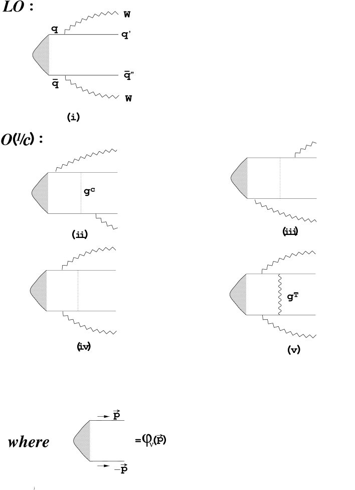
Figure 9: The diagrams which contribute to the amplitude for a nonrelativistic boundstate decaying into $q^{\prime}\bar{q}^{\prime\prime}W^{+}W^{-}$ up to ${\cal O}(1/c)$. We suppressed diagrams for ${\cal O}(\alpha_{S})$ corrections to the $qq^{\prime}W$ and $\bar{q}\bar{q}^{\prime\prime}W$ vertices.

When we vary the gauge-fixing function, additional diagrams which contribute to the ${\cal O}(1/c)$ decay amplitude are shown in Fig. 10.

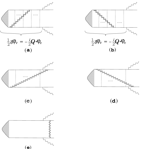
Figure 10: The diagrams which are generated by the infinitesimal variation of the gauge-fixing condition from the Coulomb gauge. The double-wavy line represents the variation of the gluon propagator $i\,\delta D_{\mu\nu}$.

Here, the double-wavy lines represent $i\,\delta D_{\mu\nu}$, where

$$i\,\delta D_{00}=-i\left(\frac{1}{k^{2}+i\epsilon}+\frac{1}{|\vec{k}|^{2}}\right)\frac{2\delta\xi\,m^{2}}{|\vec{k}|^{2}},$$ (77)

etc. Diagrams (a) and (b) can be regarded as transformations of the initial-state wave function of the leading-order diagram (i). Conversely, the diagrams (c)-(e) cannot be regarded as such, since they do not contain a $q\bar{q}$ two-body state as an intermediate state.

Using diagrammatic analysis, one may verify that the sum of all diagrams  (a)-(e) vanishes so that the total amplitude is indeed gauge independent. In fact, from diagrammatic manipulations as shown in Fig. 11 and also from similar manipulations corresponding to the diagram (b), one can show that the sum of diagrams in (a) and (b) can be regarded as the leading order diagram Fig. 9(i) with the initial state boundstate wave function $\varphi_{\nu}$ replaced by its infinitesimal transformation eq. (57).

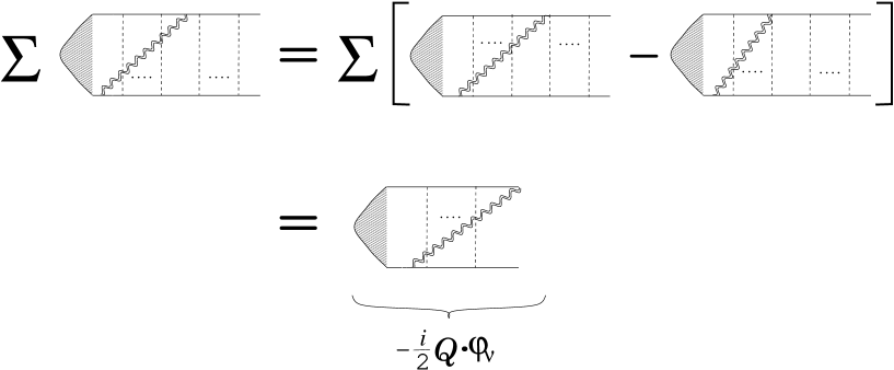
Figure 11: A diagrammatic method to show that the sum of diagrams in Fig. 10(a) can be regarded as the leading order diagram Fig. 9(i) with the initial state boundstate wave function $\varphi_{\nu}$ replaced by a half of its infinitesimal transformation $-iQ\cdot\varphi_{\nu}/2$.

Rearrangement of diagrams may be performed, for instance, using the relation

$$\frac{1}{P^{0}-2\omega_{\vec{p}}+i\epsilon}\,\left(\frac{1}{|\vec{k}|}\,\frac{1}{P^{0}-|\vec{k}|-\omega_{\vec{p}}-\omega_{\vec{p}+\vec{k}}+i\epsilon}+\frac{1}{|\vec{k}|^{2}}\right)\frac{2\delta\xi\,m^{2}}{|\vec{k}|^{2}}\,\frac{1}{P^{0}-2\omega_{\vec{p}+\vec{k}}+i\epsilon}\,$$

$$=\frac{1}{|\vec{k}|^{2}(P^{0}-|\vec{k}|-\omega_{\vec{p}}-\omega_{\vec{p}+\vec{k}}+i\epsilon)}\,\frac{\delta\xi\,m^{2}}{|\vec{k}|^{2}}\left(\frac{1}{P^{0}-2\omega_{\vec{p}}+i\epsilon}+\frac{1}{P^{0}-2\omega_{\vec{p}+\vec{k}}+i\epsilon}\right)$$ (78)

for manipulating the propagator eq. (77). On the other hand, from Fig. 12 we see that the sum of the diagrams in (c)-(e) exactly cancels the sum of (a) and (b).

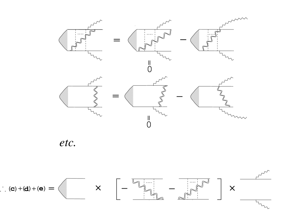
Figure 12: Examples of the diagrammatic method to show that the sum of diagrams in Fig. 10(c)-(e) exactly cancels the sum of (a) and (b).

For details of the diagrammatic analyses, see Refs. [26, 27].

According to the formal arguments in Section 4 we know how the initial-state wave function transforms and therefore we know the sum of the other diagrams (c)-(e) in order to ensure gauge independence of the total amplitude. This example demonstrates that the diagrammatic analyses are rather cumbersome since infinitely many diagrams contribute even at the lowest nontrivial order of the $1/c$ expansion.

7 Conclusion and Discussion

In this paper we analyzed gauge dependence of an effective Hamiltonian formalism that describes the nonrelativistic quark-antiquark boundstates and discussed problems of the on-shell matching procedure within this formalism. The significance of our present work may be put as follows.

We used the BRST symmetry, which is known to be a powerful tool to study QCD Green functions, to analyze the NRQCD boundstates. The arguments were supplemented by power countings of singularities of relevant diagrams to make them more explicit and detailed. Gauge dependence of the NRQCD boundstate formalism is more complex than that of usual (naive) perturbation theory since we have to deal with an infinite number of diagrams at each order of the $1/c$ expansion. (e.g. An infinite number of diagrams contribute to $H_{\rm eff}$ at ${\cal O}(1/c)$ in gauges other than the Coulomb gauge [26].) We defined $H_{\rm eff}$ naturally in the context of time-ordered perturbation theory. Then we obtained the transformation charge $Q$ of $H_{\rm eff}$, from which we could easily see gauge independence of the spectrum and obtain transformation of the boundstate wave functions. For an infinitesimal transformation from the Coulomb gauge, we calculated $Q$ directly up to ${\cal O}(1/c)$. Also we saw that, without resort to the BRST symmetry, cumbersome gauge cancellations among diagrams are necessary to show gauge independence of a decay amplitude of the boundstate. At higher orders of $1/c$, diagrammatic analyses such as what we presented in the second example or those in Refs. [26, 27] become quite intricate so that the arguments based on the BRST symmetry would become more important.

Furthermore, we showed possibilities for incorrect calculations of amplitudes involving boundstates if one uses only the on-shell $q\bar{q}$ scattering amplitude to determine $H_{\rm eff}$. These problems do not occur if we determine $H_{\rm eff}$ from the off-shell Green function ${\cal G}$, or, if we use a local NRQCD Lagrangian consistently and determine its coefficients via proper matching procedure, e.g. as in lattice calculations [37, 38]. The latter procedure has a disadvantage that one should calculate a number of amplitudes to determine all the coefficients.

Presently we still do not have at our disposal a completely systematic way to identify all the necessary contributions in computations of physical quantities of the NRQED/NRQCD boundstates at a given order of $1/c$ expansion. We believe that the formalism developed in this paper will provide useful cross checks in these computations. Now we know how a boundstate wave function or the Green function ${\cal G}$ contained in an amplitude transforms. The transformation charge $Q$ is process independent and depends only on the gauge-fixing condition, and it can be calculated directly in a perturbative expansion in $1/c$.

A possible application is to use the formalism to study gauge dependences of the diagrams involved in the calculation of the top quark momentum distribution in the $t\bar{t}$ threshold region at ${\cal O}(1/c^{2})$. It is known that at leading order the top momentum distribution is proportional to the absolute square of the wave functions of (would-be) toponium boundstates in momentum space [39]. As we saw in this paper, wave functions of boundstates are gauge dependent beyond leading order. In the second example of Section 6, we verified that this gauge dependence is cancelled by that of the final-state interaction diagrams (ii)-(v) at ${\cal O}(1/c)$. In other words, a boundstate wave function mixes with the final-state interaction diagrams by gauge transformation. This shows that the present calculations of the top momentum distribution [23] are gauge dependent, i.e. they vary if we transform the gauge infinitesimally from the Coulomb gauge, since they do not include the final-state interaction diagrams. Also the example suggests how gauge cancellations should take place in the complete amplitude at ${\cal O}(1/c^{2})$ which has not been obtained yet.

Appendix A Use of the Equation of Motion in a Local NRQCD Lagrangian

In writing down a local NRQCD Lagrangian in terms of the nonrelativistic quark ($\psi_{q}$), nonrelativistic antiquark ($\psi_{\bar{q}}$), gluon ($A_{\mu}$), ghost ($c$) and antighost ($\bar{c}$) fields, in principle one writes down all possible local interactions consistent with the rotational and BRST symmetries. In addition, one may simplify the Lagrangian using the equation of motion, and it is often convenient to eliminate all terms including $D_{0}^{n}~{}(n\geq 2)$, where $D_{\mu}=\partial_{\mu}-igA_{\mu}(x)$ is the covariant derivative. After such a simplification, the Lagrangian takes a standard form:

$${\cal L}=\psi_{q}^{\dagger}(x)\biggl{[}iD_{0}+c_{2}\frac{\vec{D}^{2}}{2m}+c_{4}\frac{\vec{D}^{4}}{8m^{3}}+c_{F}\frac{g}{2m}\vec{B}\cdot\vec{\sigma}+c_{D}\frac{g}{8m^{2}}\left(\vec{D}\cdot\vec{E}-\vec{E}\cdot\vec{D}\right)$$

$$~{}~{}~{}~{}~{}~{}~{}~{}~{}~{}+c_{S}\frac{g}{8m^{2}}i\vec{\sigma}\cdot\left(\vec{D}\times\vec{E}-\vec{E}\times\vec{D}\right)+\cdots\biggr{]}\psi_{q}(x)+(\psi_{q}\rightarrow\psi_{\bar{q}})$$

$$~{}~{}~{}~{}~{}+c_{\mbox{\scriptsize{\it 4-Fermi} }}\,\frac{g^{2}}{m^{2}}\psi_{q}^{\dagger}(x)\psi_{\bar{q}}^{\dagger}(x)\psi_{q}(x)\psi_{\bar{q}}(x)+\cdots$$

$$~{}~{}~{}~{}~{}-\frac{1}{2}{\rm tr}\left[G^{\mu\nu}G_{\mu\nu}\right].$$ (79)

We suppressed the gauge-fixing and ghost terms. One should determine the (Wilson) coefficients of local operators $c_{2}$, $c_{4}$, $c_{F}$, etc. by matching various on-shell amplitudes to those of full QCD. Furthermore, in practical applications of the NRQCD formalism, we often evaluate the correlators involving the current operators composed of the nonrelativistic quark and/or antiquark fields. The equation of motion is also used to eliminate $D_{0}^{n}$ from the current operators, and the coefficients of local operators constituting the current operators are determined by matching the on-shell amplitudes to those of full QCD.

In this appendix we prove that we may use the equation of motion appropriately in order to simplify the form of the Lagrangian. We also prove that in the evaluation of on-shell amplitudes involving current operators, the change of the Lagrangian can be compensated by local redefinitions of the current operators and that one can use the equation of motion to rewrite the current operators. It is understood that we regularize ultraviolet and infrared divergences using the dimensional regularization.

Let us start from a general local Lagrangian ${\cal L}(\psi_{q},\psi_{\bar{q}},A_{\mu},c,\bar{c})$ and add a local operator which vanishes by the equation of motion:

$${\cal L}\rightarrow{\cal L}+\psi^{\dagger}_{q}\{N,M\}\psi_{q}.$$ (80)

Here, the equation of motion for $\psi_{q}$ is denoted by

$$\frac{\delta S}{\delta\psi^{\dagger}_{q}(x)}=\left(M\psi_{q}\right)(x),~{}~{}~{}~{}~{}~{}~{}~{}~{}~{}S=\int d^{D}x\,{\cal L},$$ (81)

and $N$ denotes a local operator with $N=N^{\dagger}$, e.g. $N\,\psi_{q}=iD_{0}\psi_{q}$, $\vec{D}\,^{2}\psi_{q}$, $B\cdot\sigma\,\psi_{q}$, etc. $N$ may include the gluon field but not the quark or antiquark field. For simplicity we do not change the antiquark sector of the Lagrangian in our argument. According to eq. (80), the two-point and four-point functions change as

$$\delta\left<{0}\,\right|T\,\psi_{q}(x)\,\psi_{q}^{\dagger}(y)\left|\,{0}\,\right>=\left<{0}\,\right|T\,\psi_{q}(x)\,\psi_{q}^{\dagger}(y)\left[i\int d^{D}z\,\psi^{\dagger}_{q}(z)(\{N,M\}\psi_{q})(z)\right]\left|\,{0}\,\right>,$$ (82)

$$\delta\left<{0}\,\right|T\,\psi_{q}(x)\,\psi_{q}^{\dagger}(y)\,\psi_{\bar{q}}(x^{\prime})\,\psi_{\bar{q}}^{\dagger}(y^{\prime})\left|\,{0}\,\right>$$

$$~{}~{}~{}~{}~{}~{}~{}~{}~{}~{}~{}~{}~{}~{}~{}=\left<{0}\,\right|T\,\psi_{q}(x)\,\psi_{q}^{\dagger}(y)\,\psi_{\bar{q}}(x^{\prime})\,\psi_{\bar{q}}^{\dagger}(y^{\prime})\left[i\int d^{D}z\,\psi^{\dagger}_{q}(z)(\{N,M\}\psi_{q})(z)\right]\left|\,{0}\,\right>.$$ (83)

In order to rewrite the right-hand-side of eq. (82) one may use the Schwinger-Dyson equation

$$\left<{0}\,\right|T\,\biggl{\{}\frac{1}{2}\,\psi_{q}(x)\,[(N\psi_{q})(y)]^{\dagger}+\frac{1}{2}\,(N\psi_{q})(x)\,\psi_{q}^{\dagger}(y)+\psi_{q}(x)\,\psi_{q}^{\dagger}(y)\left[i\int d^{D}z\,N(z,z)\right]$$

$$~{}~{}~{}~{}~{}+\psi_{q}(x)\,\psi_{q}^{\dagger}(y)\left[i\int d^{D}z\,\psi^{\dagger}_{q}(z)(\{N,M\}\psi_{q})(z)\right]\biggr{\}}\left|\,{0}\,\right>=0.$$ (84)

The third term of this equation vanishes within the dimensional regularization, since $N(z,z)$ contains $\delta^{D}(0)$ and/or $[\partial_{z}^{n}\delta^{D}(z)]_{z\rightarrow 0}$ which give scaleless integrals (tadpoles). Hence, we have

$$\delta\left<{0}\,\right|T\,\psi_{q}(x)\,\psi_{q}^{\dagger}(y)\left|\,{0}\,\right>=-\left<{0}\,\right|T\,\biggl{\{}\frac{1}{2}\,\psi_{q}(x)\,[(N\psi_{q})(y)]^{\dagger}+\frac{1}{2}\,(N\psi_{q})(x)\,\psi_{q}^{\dagger}(y)\biggr{\}}\left|\,{0}\,\right>.$$ (85)

This equation shows that the change of the Lagrangian does not affect the pole mass of the quark propagator, whereas the $Z$-factor (wave function renormalization constant) varies; see Fig. 13.

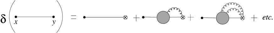
Figure 13: The diagrammatic representation of eq. (85). $\otimes$ shows the position of the local operator $N$. The pole position is not changed, while the $Z$ factor changes.

Following similar steps, one can show that the variation of the four-point function is given by

$$\delta\left<{0}\,\right|T\,\psi_{q}(x)\,\psi_{q}^{\dagger}(y)\,\psi_{\bar{q}}(x^{\prime})\,\psi_{\bar{q}}^{\dagger}(y^{\prime})\left|\,{0}\,\right>$$

$$=-\left<{0}\,\right|T\,\biggl{\{}\frac{1}{2}\,\psi_{q}(x)\,[(N\psi_{q})(y)]^{\dagger}+\frac{1}{2}\,(N\psi_{q})(x)\,\psi_{q}^{\dagger}(y)\biggr{\}}\,\psi_{\bar{q}}(x^{\prime})\,\psi_{\bar{q}}^{\dagger}(y^{\prime})\left|\,{0}\,\right>.$$ (86)

Thus, if we redefine the $Z$-factor according to eq. (85), the on-shell amplitude of the quark-antiquark scattering remains the same; see Fig. 14.

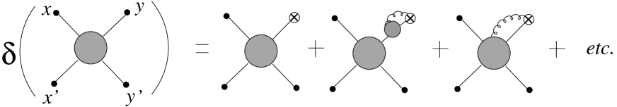
Figure 14: The diagrammatic representation of eq. (86). The first two diagrams give rise to a wave function renormalization common to Fig. 13. The third diagram is one-particle irreducible with respect to the leg with $\otimes$, hence it does not contribute to the on-shell amplitude.

Similarly the amplitudes where multiple gluons are attached to the quark-antiquark scattering can be shown to be invariant under the variation of the Lagrangian eq. (80).

Eqs. (85) and (86) also show that, when evaluating correlators involving current operators, the change of the Lagrangian can be compensated by local redefinitions of the current operators. By way of example, for a current operator which creates and annihilates a quark-antiquark pair,

$$J^{i}(x)=\psi_{q}^{\dagger}(x)\left[c_{1}^{v}\sigma^{i}+c_{2}^{v}\sigma^{i}\frac{\stackrel{{\scriptstyle\leftrightarrow}}{{D^{2}}}}{12m^{2}}+\cdots\right]\psi^{\dagger}_{\bar{q}}(x)+{\rm h.c.},$$ (87)

the on-shell amplitude calculated from the correlator $\left<{0}\,\right|T\,J^{i}(x)\,\psi_{q}(y)\psi_{\bar{q}}(z)\left|\,{0}\,\right>$ remains unchanged if we redefine the current as

$$J^{i}(x)\rightarrow J^{i}(x)+\delta J^{i}(x),$$ (88)

$$\delta J^{i}(x)=[(N\psi_{q})(x)]^{\dagger}\left[c_{1}^{v}\sigma^{i}+c_{2}^{v}\sigma^{i}\frac{\stackrel{{\scriptstyle\leftrightarrow}}{{D^{2}}}}{12m^{2}}+\cdots\right]\psi^{\dagger}_{\bar{q}}(x)+{\rm h.c.}$$ (89)

Finally we show that we may use the equation of motion in order to rewrite the current operators. One may derive the Schwinger-Dyson equation

$$\left<{0}\,\right|T\,\biggl{\{}[(\Gamma^{i}M\psi_{q})(x)]^{\dagger}\psi^{\dagger}_{\bar{q}}(x)\psi_{q}(y)\,\psi_{\bar{q}}(z)+i\Gamma^{i\dagger}(x,y)\,\psi_{\bar{q}}^{\dagger}(x)\,\psi_{\bar{q}}(z)\biggr{\}}\left|\,{0}\,\right>=0,$$ (90)

where $\Gamma^{i}$ is a local operator and may include the gluon field but not the quark or antiquark field, e.g. $\Gamma^{i}(x,y)=\sigma^{i}\delta^{D}(x-y)$, $D^{i}(x,y)$, etc. The second term does not contain the quark pole, hence it does not contribute to the on-shell amplitude. Thus, adding $[(\Gamma^{i}M\psi_{q})(x)]^{\dagger}\psi_{\bar{q}}^{\dagger}(x)+{\rm h.c.}$ to the current operator $J^{i}(x)$ does not affect the on-shell amplitude.

Appendix B Time-ordered Perturbation Theory

Here, we derive the rules for calculations of the on-shell quark-antiquark scattering amplitude in time-ordered (old-fashioned) perturbation theory. The $S$-matrix element between the eigenstates of the free Hamiltonian defined in eq. (32) with an infinite time separation (asymptotic states) is given by

$$S_{fi} = \lim_{T\rightarrow\infty}\,\left<{\vec{p},-\vec{p},\lambda,\bar{\lambda}}\,\right|e^{-iHT}\left|\,{\vec{q},-\vec{q},\lambda^{\prime},\bar{\lambda}^{\prime}}\,\right>$$ (91)

$$= \lim_{T\rightarrow\infty}\,\oint\frac{dP^{0}}{2\pi i}\,e^{-iP^{0}T}\,\left<{\vec{p},-\vec{p},\lambda,\bar{\lambda}}\,\right|\,\frac{1}{P^{0}-H+i\epsilon}\left|\,{\vec{q},-\vec{q},\lambda^{\prime},\bar{\lambda}^{\prime}}\,\right>.$$ (92)

In the integrand, we see the Green function ${\cal G}(\vec{p},\vec{q};\lambda,\bar{\lambda},\lambda^{\prime},\bar{\lambda}^{\prime};P^{0})$ introduced in eq. (31). We expand the right-hand-side in $V$, where $H=H_{0}+V$,

$$\frac{1}{P^{0}-H+i\epsilon}=\frac{1}{P^{0}-H_{0}+i\epsilon}\sum_{n=0}^{\infty}\left(V\,\frac{1}{P^{0}-H_{0}+i\epsilon}\right)^{n},$$ (93)

and insert the completeness relations in terms of the eigenstates of $H_{0}$. One readily sees that, at each order of the perturbative expansion, the free propagator poles $(P^{0}-2\omega_{\vec{p}}+i\epsilon)^{-1}$ and $(P^{0}-2\omega_{\vec{q}}+i\epsilon)^{-1}$ are attached at the both ends. Therefore, if we write

$$\left<{\vec{p},-\vec{p},\lambda,\bar{\lambda}}\,\right|\,\frac{1}{P^{0}-H+i\epsilon}\left|\,{\vec{q},-\vec{q},\lambda^{\prime},\bar{\lambda}^{\prime}}\,\right>=\frac{{\cal M}_{q\bar{q}\rightarrow q\bar{q}}(P^{0})}{(P^{0}-2\omega_{\vec{p}}+i\epsilon)(P^{0}-2\omega_{\vec{q}}+i\epsilon)}$$ (94)

and set $2\omega_{\vec{p}}=2\omega_{\vec{q}}=\sqrt{s}$, we find

$$S_{fi} = \lim_{T\rightarrow\infty}\,\oint\frac{dP^{0}}{2\pi i}\,e^{-iP^{0}T}\,\left(\frac{1}{P^{0}-\sqrt{s}+i\epsilon}\right)^{2}{\cal M}_{q\bar{q}\rightarrow q\bar{q}}(P^{0}).$$ (95)

Suppose ${\cal M}_{q\bar{q}\rightarrow q\bar{q}}(P^{0})$ is regular inside the integration contour. Then

$$S_{fi} = \lim_{T\rightarrow\infty}\,\frac{\partial}{\partial P^{0}}\,\{e^{-iP^{0}T}\,{\cal M}_{q\bar{q}\rightarrow q\bar{q}}(P^{0})\}\biggr{|}_{P^{0}\rightarrow\sqrt{s}}$$ (96)

$$= \lim_{T\rightarrow\infty}\,e^{-i\sqrt{s}T}\{{\cal M}_{q\bar{q}\rightarrow q\bar{q}}^{\prime}(\sqrt{s})-iT\,{\cal M}_{q\bar{q}\rightarrow q\bar{q}}(\sqrt{s})\}.$$ (97)

The second term in the last line represents the dominant term as $T\rightarrow\infty$. Taking into account the irregularity of ${\cal M}_{q\bar{q}\rightarrow q\bar{q}}(P^{0})$, we obtain additional terms which are subleading in comparison to the second term of eq. (97) as $T\rightarrow\infty$. Thus, we obtain the reduction formula eq. (50) as well as the rules for calculations of the scattering amplitude in time-ordered perturbation theory, as explained in Sec. 4.

Following similar steps, one can show that in general the Green function ${\cal G}$ appears as an intermediate matrix element when one evaluates a transition amplitude involving contributions from the quark-antiquark boundstates using time-ordered perturbation theory.

Appendix C Absence of Boundstate Poles in Eq. (46)

We show that the state given by eq. (46) cannot accomodate a pole which is degenerate with any of the quark-antiquark boundstate poles, $(P^{0}-M_{\nu}+i\epsilon)^{-1}$. We first note that $Q_{B}$ and $\delta O$ have the ghost number $+1$ and $-1$, respectively. Suppose this state contains some of these boundstate poles. Then, the matrix element composed of this state should have a power counting in terms of $\alpha_{S}$ and $\beta$ as

$$\left<{\vec{p},-\vec{p},\lambda,\bar{\lambda}}\,\right|\delta O\,\frac{1}{P^{0}-H+i\epsilon}\,iQ_{B}\,\left|\,{\vec{q},-\vec{q},\lambda^{\prime},\bar{\lambda}^{\prime}}\,\right>$$

$$~{}~{}~{}~{}~{}~{}~{}~{}~{}~{}~{}~{}~{}~{}~{}~{}~{}~{}~{}~{}\sim\beta^{n_{0}}\sum_{n}c_{n}\,(\alpha_{S}/\beta)^{n}\times\biggl{[}1+{\cal O}(1/c)\biggr{]}$$ (98)

for some $n_{0}$, since $P^{0}-M_{\nu}=[1-{C_{F}^{2}(\alpha_{S}/\beta)^{2}}/{4l^{2}}]\,m\beta^{2}$ at leading order. It is known that the diagrams which can have the leading power counting $(\alpha_{S}/\beta)^{n}$ are only the uncrossed ladder diagrams; see Section 3. Therefore the diagrams which can contribute to $\beta^{n_{0}}\,(\alpha_{S}/\beta)^{n}$ for $n\gg n_{0}$ are only those diagrams where a ghost is connected to one of the uncrossed ladders of $q\bar{q}$ with a finite number [$\hbox{ \raise 3.0pt\hbox to0.0pt{$<$}\raise-3.0pt\hbox{$\sim$} }{\cal O}(n_{0})$] of lines; see Fig. 15.

Figure 15: Typical diagrams which have power countings $\beta^{n_{0}}\,(\alpha_{S}/\beta)^{n}$ for $n\gg n_{0}$. The ghost is connected with the uncrossed ladders of $q\bar{q}$ with a finite number [$\hbox{ \raise 3.0pt\hbox to0.0pt{$<$}\raise-3.0pt\hbox{$\sim$} }{\cal O}(n_{0})$] of lines.

After integrating over the loop momenta, there remains no pole in the $P^{0}$-dependence of the sum of the diagrams, in the same way that a usual one-loop diagram does not exhibit a pole but rather contains branch point(s); cf. eq. (75).

We may restate it differently. If a ghost and a nonrelativistic $q\bar{q}$ pair should constitute a boundstate, intuitively the sum of the ladder diagrams with multiple gluon exchanges between the ghost and $q\bar{q}$ pair may exhibit a boundstate pole. Since the coupling of ghost and gluon is suppressed by powers of $\beta$, the binding energy of the boundstate should scale differently from (have more powers of $\alpha_{S}$ than) the Coulomb binding energies (if the boundstate should exist at all).

References

- [1] W. Caswell and G. Lepage, Phys. Lett. B167, 437 (1986).
- [2] G. Bodwin, E. Braaten and G. Lepage, Phys. Rev. D51, 1125 (1995); Erratum ibid. D55, 5853 (1997).
- [3] P. Labelle, Phys. Rev. D58, 093013 (1998).
- [4] M. Luke and A. Manohar, Phys. Rev. D55, 4129 (1997).
- [5] B. Grinstein and I. Rothstein, Phys. Rev. D57, 78 (1998).
- [6] M. Luke and M. Savage, Phys. Rev. D57, 413 (1998).
- [7] A. Pineda and J. Soto, Nucl. Phys. B (Proc. Suppl.) 64, 428 (1998); Phys. Rev. D59, 016005 (1998).
- [8] M. Beneke and V. Smirnov, Nucl. Phys. B522 321 (1998).
- [9] H. Griesshammer, Phys. Rev. D58, 094027 (1998).
- [10] M. Luke, A. Manohar and I. Rothstein, hep-ph/9910209.
- [11] A. Hoang, M. Smith, T. Stelzer and S. Willenbrock, Phys. Rev. D59, 114014 (1999); M. Beneke, Phys. Lett. B434, 115 (1998).
- [12] T. Kinoshita and M. Nio, Phys. Rev. D53, 4909 (1996); Phys. Rev. D55, 7267 (1997).
- [13] G. Adkins, R. Fall and P. Mitrikov, Phys. Rev. Lett. 79, 3383 (1997); A. Hoang, P. Labelle and S. Zebarjad, Phys. Rev. Lett. 79, 3387 (1997); hep-ph/9909495.
- [14] A. Czarnecki, K. Melnikov and A. Yelkhovsky, Phys. Rev. Lett. 82, 311 (1999); Phys. Rev. A59, 4316 (1999); Phys. Rev. Lett. 83, 1135 (1999).
- [15] M. Peter, Phys. Rev. Lett. 78, 602 (1997); Nucl. Phys. B501 471 (1997); Y. Schröder, Phys. Lett. B447, 321 (1999).
- [16] A. Pineda and F. Ynduráin, Phys. Rev. D58, 094022 (1998); hep-ph/9812371.
- [17] A. Hoang and T. Teubner, Phys. Rev. D58, 114023 (1998); K. Melnikov and A. Yelkhovsky, Nucl. Phys. B528, 59 (1998).
- [18] A. Hoang, Phys. Rev. D59, 014039 (1999).
- [19] K. Melnikov and A. Yelkhovsky, Phys. Rev. D59, 114009 (1999); A. Penin and A. Pivovarov, Nucl. Phys. B549, 217 (1999); hep-ph/9904278.
- [20] O. Yakovlev, hep-ph/9808463.
- [21] N. Brambilla, A. Pineda, J. Soto and A. Vairo, Phys. Rev. D60, 091502 (1999); hep-ph/9907240; hep-ph/9910238.
- [22] M. Beneke, A. Signer and V. Smirnov, hep-ph/9903260.
- [23] T. Nagano, A. Ota and Y. Sumino, hep-ph/9903498; A. Hoang and T. Teubner, hep-ph/9904468.
- [24] B. Kniehl and A. Penin, hep-ph/9907489.
- [25] G. Bodwin and D. Yennie, Phys. Rep. 43, 267 (1978).
- [26] S. Love, Ann. of Phys. 113, 153 (1978).
- [27] G. Feldman, T. Fulton and D. Heckathorn, Nucl. Phys. B167, 364 (1980); Nucl. Phys. B174, 89 (1980).
- [28] M. Luscher and P. Weisz, Comm. Math. Phys. 97, 59 (1985); Erratum ibid. 98, 433 (1985).
- [29] S. Scherer and H. Fearing, Phys. Rev. D52, 6445 (1995).
- [30] T. Kugo and I. Ojima, Phys. Lett. 73B, 459 (1978); Prog. Theor. Phys. Suppl. 66, 1 (1979); N. Nakanishi and I. Ojima, “Covariant Operator Formalism of Gauge Theories and Quantum Gravity”, (World Scientific Lecture Notes in Physics Vol. 27, 1990).
- [31] D. Lurié, A. MacFarlane and Y. Takahashi, Phys. Rev. 140B, 1091 (1965).
- [32] M. Braun, Sov. Phys. JETP 27, 652 (1968).
- [33] T. Appelquist and H. Politzer, Phys. Rev. Lett. 34, 43 (1975); Phys. Rev. D12, 1404 (1975).
- [34] F. Halzen and A. Martin, “Quarks & Leptons”, (John Wiley & Sons, 1984).
- [35] D. Heckathorn, Nucl. Phys. B156, 328 (1979).
- [36] Y. Sumino, PhD thesis, University of Tokyo 1993 (unpublished); M. Peter and Y. Sumino, Phys. Rev. D57, 6912 (1998).
- [37] B. Thacker and G. Lepage, Phys. Rev. D43, 196 (1991); G. Lepage, L. Magnea and C. Nakhleh, Phys. Rev. D46, 4052 (1992).
- [38] A. Khan, J. Shigemitsu, S. Collins, C. Davies, C. Morningstar and J. Sloan, Phys. Rev. D56, 7012 (1997); K. Ishikawa, H. Matsufuru, T. Onogi, N. Yamada and S. Hashimoto, Phys. Rev. D56, 7028 (1997).
- [39] Y. Sumino, K. Fujii, K. Hagiwara, H. Murayama, and C.-K. Ng, Phys. Rev. D47, 56 (1993); M. Jeżabek, J.H. Kühn and T. Teubner, Z. Phys. C56, 653 (1992); M. Jeżabek and T. Teubner, Z. Phys. C59, 669 (1993).