UM-TH-99-08

October 1999

Momentum expansion of massive two-loop Feynman graphs around a finite value
Adrian Ghinculov and York-Peng Yao

Randall Laboratory of Physics, University of Michigan,
Ann Arbor, Michigan 48109-1120, USA

We give an algorithm for obtaining expansions of massive two-loop Feynman graphs in powers of the external momentum around a finite, nonzero value of the momentum. This is based on our general two-loop formalism to reduce massive two-loop graphs with renormalizable interactions into a standard set of special functions. After the algebraic reduction, the final results are obtained by numerical integration. We apply the expansion algorithm to treat the top-dependent corrections of ${\cal O}(g^{2}\alpha_{s})$ to the $b$ quark self-energy and extract its momentum expansion on-shell.

Abstract

We give an algorithm for obtaining expansions of massive two-loop Feynman graphs in powers of the external momentum around a finite, nonzero value of the momentum. This is based on our general two-loop formalism to reduce massive two-loop graphs with renormalizable interactions into a standard set of special functions. After the algebraic reduction, the final results are obtained by numerical integration. We apply the expansion algorithm to treat the top-dependent corrections of ${\cal O}(g^{2}\alpha_{s})$ to the $b$ quark self-energy and extract its momentum expansion on-shell.

Analyses of electroweak data based on two-loop radiative corrections have become necessary due to the precision level attained already. The experimental precision is expected to reach even deeper at the next generation of colliders in the near future. This motivated in recent years an enormous amount of work in handling massive two-loop Feynman graphs. In its general form, this is a notoriously difficult problem. The essence of the difficulties is that these graphs usually lead to unknown special functions.

In a previous paper [1] we gave a general formalism for evaluating two-loop Feynman diagrams for arbitrary kinematical variables, based on analytical-numerical methods. By using this framework, the internal mass structure and the external kinematics of the physical process under consideration are fully respected. Radiative corrections are obtained at the end by high accuracy numerical integration.

In this letter we would like to discuss the use of our general massive two-loop framework of ref. [1] for obtaining external momentum expansions around a finite value. There are situations where such momentum expansions around a finite value are needed in the evaluation of radiative corrections, most notably for mass and wave function renormalization constants. However, we note that the algorithm described in this letter can produce the full momentum expansion around a finite value; it works systematically for terms of higher order in the momentum as well.

We refer to the important process $Z\rightarrow b\bar{b}$ [2]–[10] to illustrate in some detail the technical aspects. A piece of the analysis of this process involves the calculation of the $b$ quark wave function renormalization on-shell. This is a good example for the general problem of expanding an amplitude at a certain kinematical point, and we would like to use this short communication to treat this problem. Let us begin with a broader discussion.

In a perturbative calculation, one is faced with a set of momentum space integrals, where the external momenta appear at various parts of the integrands. The dependence on the invariants $\{s\}$ constructed from these external momenta is implicit at this stage. One may introduce Feynman parameters and integrate over the internal momenta, the result of which will be some Feynman parameter integrals, where the dependence on $\{s\}$ is made explicit. In principle, one can then expand the integrands around some fixed values $\{s_{0}\}$.

At the one-loop level, this procedure can be easily followed, since the one-loop scalar integrals are relatively simple. At higher loops, there are at least two complications to follow this route. First of all, due to the proliferation of diagrams, one must have a systematic procedure. The Feynman parameter integrals due to different diagrams are most likely quite different, and for avoiding errors it is desirable to have a uniform treatment for all the graphs, the number of which can be quite formidable. Secondly, the integrations over the Feynman parameters must be feasible, in the sense of fast convergence and high precision.

At the two-loop level, we developed in ref. [1] a framework by which all two-loop processes with general renomalizable interactions can be written as a small set of Feynman parameter integrations over ten special functions $h_{i}$. It would seem that an expansion around $\{s_{0}\}$ should be an easy task. However, this is not as straightforward as it appears, because the scalar integrals are made of functions of $\{s\}$, and a brute force expansion will result in rather unwieldy expressions. What is needed is a procedure to expand the momentum integrals around $\{s_{0}\}$ before the momentum integration, in such a way that the final product is still a linear combination of the ten scalar integrals. This will greatly facilitate systematic and rapidly convergent numerical work. We shall describe such a procedure in the following, for two-point functions.

Our method is based on an expansion of individual propagators around a finite external momentum. In the following, we use a simple one-loop example in QED to show how the procedure is carried out. Afterwards we extend it to two-loop and apply it to the $b$ quark self-energy, and derive the wave function renormalization constant as needed for the $Z\rightarrow b\bar{b}$ process.

Let us consider the self-energy of a fermion (the discussion for the bosonic case proceeds similarly):

$$\Sigma(k)=[A(k^{2})+\gamma_{5}A_{5}(k^{2})]\gamma\cdot k+B(k^{2})+\gamma_{5}B_{5}(k^{2})\;\;\;.$$ (1)

We want to obtain an expansion of this expression in powers of $k^{2}$ around a finite value $k^{2}=k_{0}^{2}$. Given a set of Feynman graphs of a certain loop order, in the case when one is able to evaluate them analytically, it is of course straightforward to perform a momentum expansion of the functions in the above expression.

However, when several finite masses and momenta are involved, in general such analytical solutions are not available beyond one loop. Instead, we can obtain systematically an expansion of the integrands by expanding the individual propagators which contain the external momentum $k$. We introduce a deviation $\Delta_{\mu}$ of the external momentum $k_{\mu}$ around the finite expansion point $k_{0\mu}$:

$$k_{\mu}=k_{0\mu}+\Delta_{\mu}$$ (2)

such that the deviation is orthogonal to $k_{0}$, $\Delta\cdot k_{0}=0$. We have the freedom to make this specific choice for $\Delta$ because the coefficients in the expansion are independent of the direction of differentiation. Squaring $k_{\mu}$, one obtains $\Delta^{2}=k^{2}-k_{0}^{2}$.

When writing down the integrand of a Feynman graph, the numerator is already a polynomial of the external momentum $k$, while the propagators containing $k$ can be expanded around $k_{0}$:

$$\frac{1}{(p+k)^{2}-m^{2}}=\frac{1}{(p+k_{0})^{2}-m^{2}}-\frac{\Delta^{2}+2p\cdot\Delta}{[(p+k_{0})^{2}-m^{2}]^{2}}+\frac{[\Delta^{2}+2p\cdot\Delta]^{2}}{[(p+k_{0})^{2}-m^{2}]^{3}}-\dots$$ (3)

where $p$ is a loop integration momentum, and we used the fact that $\Delta\cdot k_{0}=0$.

Thus the dependence of the integrand on the deviation $\Delta$ becomes polynomial. For each order in $\Delta$ one can further use the algorithm described in ref. [1] to calculate directly the desired coefficient. One obtains directly the expansion of the functions $A(k^{2})$, $A_{5}(k^{2})$, $B(k^{2})$ and $B_{5}(k^{2})$. In particular, one is able to extract directly the mass and wave function renormalization counterterms.

As a simple example, let us look at the electron mass operator at one-loop order in quantum electrodynamics. The momentum space integral in Feynman gauge is :

$$i\Sigma(k)=e^{2}\int{\frac{d^{n}p}{(2\pi)^{n}}\frac{\gamma^{\mu}[\gamma\cdot(p+k)+m]\gamma_{\mu}}{[(p+k)^{2}-m^{2}](p^{2}-m_{\gamma}^{2})}},$$ (4)

in which $m$ is the electron mass, and $m_{\gamma}$ is the photon mass regulator. The conventional way of introducing a Feynman parameter $x$ and integrating over $p$ gives:

$$\Sigma(k)={e^{2}\over(4\pi)^{\frac{n}{2}}}\int dx\Gamma(-{\epsilon\over 2})(m_{k}^{2})^{\epsilon\over 2}[nm+(2-n)(1-x)\gamma\cdot k],$$ (5)

where $m_{k}^{2}=xm^{2}+(1-x)m_{\gamma}^{2}-x(1-x)k^{2}$, and $n=4+\epsilon$. This can be expanded in $\epsilon$, and after a $\overline{MS}$ subtraction we have:

$$\Sigma(k) = -\frac{e^{2}}{16\pi^{2}}\int dx\left\{m[2x+2(1+x)\ln{(m_{x}^{2})}]\right.$$ (6)

$$-(\gamma\cdot k-m)\left[(1-x)[2+2\ln{(m_{x}^{2})}]+\frac{4m^{2}x(1-x^{2})}{m_{x}^{2}}\right]$$

$$\left.+{\cal O}((\gamma\cdot k-m)^{2})\right\}\;\;\;,$$

with $m_{x}^{2}=x^{2}m^{2}+(1-x)m_{\gamma}^{2}$.

In the second approach we just proposed, we expand the electron propagator according to eq. 3, and write:

$$\Sigma=\Sigma_{0}+\Sigma_{1}+\Sigma_{2}+{\cal O}(\Delta^{3})\;\;\;,$$ (7)

where ($p=p^{\prime}-xk_{0}$):

$$i\Sigma_{0} = {e^{2}\over(2\pi)^{4}}\int dxd^{n}p^{\prime}{nm+(2-n)\gamma\cdot[(1-x)k_{0}+\Delta]\over(p^{\prime 2}-m_{x}^{2})^{2}}$$

$$i\Sigma_{1} = -2{e^{2}\over(2\pi)^{4}}\int dxd^{n}p^{\prime}x{2({2-n\over n})p^{\prime 2}\gamma\cdot\Delta+\Delta^{2}[nm+(2-n)(1-x)\gamma\cdot k_{0}]\over(p^{\prime 2}-m_{x}^{2})^{3}}$$

$$i\Sigma_{2} = 3{e^{2}\over(2\pi)^{4}}\int dxx^{2}d^{n}p^{\prime}4p^{\prime 2}\Delta^{2}{m+\left(\frac{2-n}{n}\right)(1-x)\gamma\cdot k_{0}\over(p^{\prime 2}-m_{x}^{2})^{4}}\;\;\;.$$ (8)

After making a $\overline{MS}$ subtraction in eqs. 8 and adding up the results, we regain the result in eq. 6. This confirms the consistency of the expansion procedure. Note the terms $\gamma\cdot\Delta$ in eqs. 8, which combine with the $\gamma\cdot k_{0}$ terms to produce $\gamma\cdot k$ terms in eq. 6, as they must. This feature can be used as a check.

This expansion procedure can be extended directly at two-loop level. The resulting coefficients of the $\Delta$ expansion can be further decomposed into $h_{i}$ functions and evaluated numerically along the lines of ref. [1].

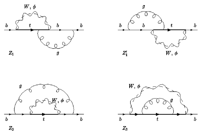
Figure 1: The two-loop Feynman graphs which contribute to the top-dependent $b$ quark self-energy at ${\cal O}(g^{2}\alpha_{s})$.

As an example, we give in figure 1 the two-loop Feynman graphs which contribute to the top-dependent $b$ quark self-energy at ${\cal O}(g^{2}\alpha_{s})$. The wave function renormalization constant derived from this two-point function contributes to the important process $Z\rightarrow b\bar{b}$ [2]–[10].

By expanding the propagators according to eq. 3, and identifying the terms according to their power of $\Delta$, one can obtain the momentum expansion of the functions $A(k^{2})$, $A_{5}(k^{2})$, $B(k^{2})$ and $B_{5}(k^{2})$ of eq. 1 on-shell, i.e. around $k_{0}^{2}=m_{b}^{2}$. The wave function renormalization contribution involves $A(m_{b}^{2})$, $A_{5}(m_{b}^{2})$, $B^{\prime}(m_{b}^{2})$, $B^{\prime}_{5}(m_{b}^{2})$, $A^{\prime}(m_{b}^{2})$, and $A_{5}^{\prime}(m_{b}^{2})$, where the prime denotes the derivative with respect to the momentum squared ($\partial/\partial k^{2}$).

Figure 2: Terms in the momentum expansion of the functions $A(k^{2})$, $A_{5}(k^{2})$, $B(k^{2})$ and $B_{5}(k^{2})$ of eq. 1 for the $b$ quark self-energy (figure 1). The prime denotes differentiation with respect to the external momentum, $\partial/\partial k^{2}$. The expansion is performed on-shell ($k^{2}=m_{b}^{2}$). UV divergencies are subtracted by MS. We plot the results for a range of the top mass $m_{t}$ and of the gluon infrared regulator $m_{g}$. An overall coupling constant factor of $\alpha_{s}(g/2\sqrt{2})^{2}$ and a $4/3$ colour factor are understood.

After isolating from the diagrams the $A(m_{b}^{2})$, $A_{5}(m_{b}^{2})$, $B^{\prime}(m_{b}^{2})$, $B^{\prime}_{5}(m_{b}^{2})$, $A^{\prime}(m_{b}^{2})$, and $A_{5}^{\prime}(m_{b}^{2})$, contributions, we use the general algorithm of ref. [1] to evaluate them. We used $M_{W}=80.41$ GeV, $m_{b}=4.2$ GeV, and $\sin^{2}\theta_{W}=.231$. To regularize the infrared singularities, we introduced a mass regulator for the gluon. This being an ${\cal O}(g^{2}\alpha_{s})$ correction, the use of a gluon mass regulator is legitimate. When calculating a physical process, the gluon mass singularities are canceled by those from real emission diagrams; the net effect is to replace the mass regulator by the experimental energy resolution. The final results are given in figure 2 for a range of the top mass. Here we used MS to treat the ultraviolet infinities.

At this point we note that in ref. [8] the $b$ quark self-energy is given in the massles $b$ limit as a large top mass expansion up to the 10^th order. A direct comparizon of these results with ours is difficult because ref. [8] uses dimensional regularization for handling the infrared divergencies, while we have a gluon mass regulator. However, we checked that in the massles $b$ limit our result for the self-energy contains only a left-handed component (i.e. $A(k^{2})=A_{5}(k^{2})$, $B(k^{2})=B_{5}(k^{2})\rightarrow 0$ in eq. 1), in agreement with the results of ref. [8].

To conclude, we have shown how momentum expansions of massive two-loop diagrams around a finite external momentum can be obtained systematically and evaluated with the general methods which we introduced previously in ref. [1]. Such momentum expansions are needed in the computation of radiative corrections, for instance in the evaluation of wave function renormalization constants. The method we described in this letter has the advantage that provides a uniform treatment of all two-loop topologies, and is suitable for implementation in a computer algebra program for an automatic treatment. The final result of the computer algebra program is a set of special functions $h_{i}$ which are evaluated further numerically.

Acknowledgement

This work was partially supported by the US Department of Energy (DOE).

References

- [1] A. Ghinculov and Y.-P. Yao, Nucl. Phys. B516 (1998) 385.
- [2] J. Fleischer, O.V. Tarasov, F. Jegerlehner, P. Raczka, Phys. Lett. B293 (1992) 437.
- [3] G. Buchalla, A.J. Buras, Nucl. Phys. B398 (1993) 285.
- [4] G. Degrassi, Nucl. Phys. B407 (1993) 271.
- [5] K.G. Chetyrkin, A. Kwiatkowski, M. Steinhauser, Mod. Phys. Lett. A8 (1993) 2785.
- [6] A. Kwiatkowski, M. Steinhauser, Phys. Lett. B344 (1995) 359.
- [7] R. Harlander, T. Seidensticker, M. Steinhauser, Phys. Lett. B426 (1998) 125.
- [8] J. Fleischer, F. Jegerlehner, M. Tentyukov, O.L. Veretin, Phys. Lett. B459 (1999) 625.
- [9] G. Degrassi, Paolo Gambino, hep-ph/9905472 (1999).
- [10] A. Ghinculov and Y.-P. Yao, in preparation.