Electroweak Precision Tests

Abstract

Precision measurements of electroweak observables provide stringent tests of the Standard Model structure and an accurate determination of its parameters. An overview of the present experimental status is presented.

FTUV/99-69
IFIC/99-72

1 INTRODUCTION

The Standard Model (SM) constitutes one of the most successful achievements in modern physics. It provides a very elegant theoretical framework, which is able to describe all known experimental facts in particle physics. A detailed description of the SM and its impressive phenomenological success can be found in Refs. [1] and [2], which discuss the electroweak and strong sectors, respectively.

The high accuracy achieved by the most recent experiments allows to make stringent tests of the SM structure at the level of quantum corrections. The different measurements complement each other in their different sensitivity to the SM parameters. Confronting these measurements with the theoretical predictions, one can check the internal consistency of the SM framework and determine its parameters.

The following sections provide an overview of our present experimental knowledge on the electroweak couplings. A brief description of some classical QED tests is presented in Section 2. The leptonic couplings of the $W^{\pm}$ bosons are analyzed in Section 3, where the tests on lepton universality and the Lorentz structure of the $l^{-}\to\nu_{l}l^{\prime-}\bar{\nu}_{l^{\prime}}$ transition amplitudes are discussed. Section 4 describes the status of the neutral–current sector, using the latest experimental results reported by LEP and SLD. Some summarizing comments are finally given in Section 5.

2 QED

The most stringent QED test [3, 4, 5, 6, 7, 8, 9, 10, 11, 12, 13] comes from the high–precision measurements [14] of the $e$ and $\mu$ anomalous magnetic moments $a_{l}^{\gamma}\equiv(g_{l}-2)/2$:

$$a_{e}^{\gamma} \!\!\!= \!\!\!\left\{\!\begin{array}[]{cc}(115\,965\,215.4\pm 2.4)\times 10^{-11}&(\mbox{\rm Theory})\\ (115\,965\,219.3\pm 1.0)\times 10^{-11}&(\mbox{\rm Exp.})\end{array}\right.$$ (3)

$$a_{\mu}^{\gamma} \!\!\!= \!\!\!\left\{\!\begin{array}[]{cc}(1\,165\,916.0\pm 0.7)\times 10^{-9}&(\mbox{\rm Theory})\\ (1\,165\,923.0\pm 8.4)\times 10^{-9}&(\mbox{\rm Exp.})\end{array}\right.$$ (6)

The impressive agreement between theory and experiment (at the level of the ninth digit for $a_{e}^{\gamma}$) promotes QED to the level of the best theory ever build by the human mind to describe nature. Hypothetical new–physics effects are constrained to the ranges $|\delta a_{e}^{\gamma}|<0.9\times 10^{-10}$ and $|\delta a_{\mu}^{\gamma}|<2.4\times 10^{-8}$ (95% CL).

To a measurable level, $a_{e}^{\gamma}$ arises entirely from virtual electrons and photons; these contributions are known [4] to $O(\alpha^{4})$. The sum of all other QED corrections, associated with higher–mass leptons or intermediate quarks, only amounts to $+(0.4366\pm 0.0042)\times 10^{-11}$, while the weak interaction effect is a tiny $+0.0030\times 10^{-11}$; these numbers [4] are well below the present experimental precision. The theoretical error is dominated by the uncertainty in the input value of the electromagnetic coupling $\alpha$. In fact, turning things around, one can use $a_{e}^{\gamma}$ to make the most precise determination of the fine structure constant [4, 5]:

$$\alpha^{-1}=137.03599959\pm 0.00000040\,.$$ (7)

The resulting accuracy is one order of magnitude better than the usually quoted value [14] $\alpha^{-1}=137.0359895\pm 0.0000061$.

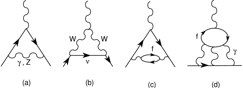
Figure 1: Some Feynman diagrams contributing to $a_{l}^{\gamma}$.

The anomalous magnetic moment of the muon is sensitive to virtual contributions from heavier states; compared to $a_{e}^{\gamma}$, they scale as $m_{\mu}^{2}/m_{e}^{2}$. The main theoretical uncertainty on $a_{\mu}^{\gamma}$ has a QCD origin. Since quarks have electric charge, virtual quark–antiquark pairs can be created by the photon leading to the so–called hadronic vacuum polarization corrections to the photon propagator (Figure 1.c). Owing to the non-perturbative character of QCD at low energies, the light–quark contribution cannot be reliably calculated at present; fortunately, this effect can be extracted from the measurement of the cross-section $\sigma(e^{+}e^{-}\to\mbox{\rm hadrons})$ at low energies, and from the invariant–mass distribution of the final hadrons in $\tau$ decays [13]. The large uncertainties of the present data are the dominant limitation to the achievable theoretical precision on $a_{\mu}^{\gamma}$. It is expected that this will be improved at the DA$\Phi$NE $\Phi$ factory, where an accurate measurement of the hadronic production cross-section in the most relevant kinematical region is expected [15]. Additional QCD uncertainties stem from the (smaller) light–by–light scattering contributions, where four photons couple to a light–quark loop (Figure 1.d); these corrections are under active investigation at present [10, 11, 12].

The improvement of the theoretical $a_{\mu}^{\gamma}$ prediction is of great interest in view of the new E821 experiment [16], presently running at Brookhaven, which aims to reach a sensitivity of at least $4\times 10^{-10}$, and thereby observe the contributions from virtual $W^{\pm}$ and $Z$ bosons [5, 6, 7] ($\delta a_{\mu}^{\gamma}|_{\mbox{\rm\scriptsize weak}}\sim 15\times 10^{-10}$). The extent to which this measurement could provide a meaningful test of the electroweak theory depends critically on the accuracy one will be able to achieve pinning down the QCD corrections.

3 LEPTONIC CHARGED–CURRENT COUPLINGS

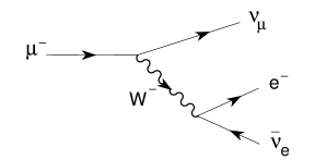
Figure 2: $\mu$–decay diagram.

The simplest flavour–changing process is the leptonic decay of the $\mu$, which proceeds through the $W$–exchange diagram shown in Figure 2. The momentum transfer carried by the intermediate $W$ is very small compared to $M_{W}$. Therefore, the vector–boson propagator reduces to a contact interaction. The decay can then be described through an effective local 4–fermion Hamiltonian,

$${\cal H}_{\mbox{\rm\scriptsize eff}}\,=\,{G_{F}\over\sqrt{2}}\left[\bar{e}\gamma^{\alpha}(1-\gamma_{5})\nu_{e}\right]\,\left[\bar{\nu}_{\mu}\gamma_{\alpha}(1-\gamma_{5})\mu\right]\,,$$ (8)

where

$${G_{F}\over\sqrt{2}}={g^{2}\over 8M_{W}^{2}}$$ (9)

is called the Fermi coupling constant. $G_{F}$ is fixed by the total decay width,

$${1\over\tau_{\mu}}={G_{F}^{2}m_{\mu}^{5}\over 192\pi^{3}}\,\left(1+\delta_{\mbox{\rm\scriptsize RC}}\right)\,f\left(m_{e}^{2}/m_{\mu}^{2}\right)\,,$$ (10)

where $\,f(x)=1-8x+8x^{3}-x^{4}-12x^{2}\ln{x}$, and $\delta_{\mbox{\rm\scriptsize RC}}=-0.0042$ takes into account the leading higher–order corrections [17, 18]. The measured $\mu$ lifetime [14], $\tau_{\mu}=(2.19703\pm 0.00004)\times 10^{-6}$ s, implies the value

$$G_{F} = (1.16637\pm 0.00001)\times 10^{-5}\>\mbox{\rm GeV}^{-2}$$ (11)

$$\approx (293\>\mbox{\rm GeV})^{-2}\,.$$

Figure 3: $\tau$–decay diagram.

The leptonic $\tau$ decay widths $\tau^{-}\to l^{-}\bar{\nu}_{l}\nu_{\tau}$  ($l=e,\mu$) are also given by Eq. (10), making the appropriate changes for the masses of the initial and final leptons. Using the value of $G_{F}$ measured in $\mu$ decay, one gets a relation between the $\tau$ lifetime and leptonic branching ratios [19]:

$$B_{\tau\to e} = {B_{\tau\to\mu}\over 0.972564\pm 0.000010}$$ (12)

$$= {\tau_{\tau}\over(1.6321\pm 0.0014)\times 10^{-12}\,\mbox{\rm s}}\,.$$

The errors reflect the present uncertainty of $0.3$ MeV in the value of $m_{\tau}$.

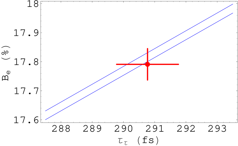
Figure 4: Relation between $B_{\tau\to e}$ and $\tau_{\tau}$. The band corresponds to the SM prediction in Eq. (12).

The measured ratio $B_{\tau\to\mu}/B_{\tau\to e}=0.974\pm 0.004$ is in perfect agreement with the predicted value. As shown in Figure 4, the relation between $B_{\tau\to e}$ and $\tau_{\tau}$ is also well satisfied by the present data. The experimental precision (0.3%) is already approaching the level where a possible non-zero $\nu_{\tau}$ mass could become relevant; the present bound [19] $m_{\nu_{\tau}}<18.2$ MeV (95% CL) only guarantees that such effect is below 0.08%.

These measurements test the universality of the $W$ couplings to the leptonic charged currents. Allowing the coupling $g$ to depend on the considered lepton flavour (i.e. $g_{e}$, $g_{\mu}$, $g_{\tau}$), the $B_{\tau\to\mu}/B_{\tau\to e}$ ratio constrains $|g_{\mu}/g_{e}|$, while $B_{\tau\to e}/\tau_{\tau}$ provides information on $|g_{\tau}/g_{\mu}|$. The present results [19] are shown in Tables 3, 3 and 3, together with the values obtained from the ratios $R_{\pi\to e/\mu}\equiv\Gamma(\pi^{-}\to e^{-}\bar{\nu}_{e})/\Gamma(\pi^{-}\to\mu^{-}\bar{\nu}_{\mu})$ and $R_{\tau/P}\equiv\Gamma(\tau^{-}\to\nu_{\tau}P^{-})/\Gamma(P^{-}\to\mu^{-}\bar{\nu}_{\mu})\,$ [$P=\pi,K$], from the comparison of the $\sigma\cdot B$ partial production cross-sections for the various $W^{-}\to l^{-}\bar{\nu}_{l}$ decay modes at the $p\bar{p}$ colliders, and from the most recent LEP2 measurements of the leptonic $W^{\pm}$ branching ratios.

Table 1: Present constraints on $|g_{\mu}/g_{e}|$.

	$|g_{\mu}/g_{e}|$
$B_{\tau\to\mu}/B_{\tau\to e}$	$1.0009\pm 0.0022$
$B_{\pi\to e}/B_{\pi\to\mu}$	$1.0017\pm 0.0015$
$\sigma\cdot B_{W\to\mu/e}$   ($p\bar{p}$)	$0.98\pm 0.03$
$B_{W\to\mu/e}$ (LEP2)	$1.002\pm 0.016$

Table 2: Present constraints on $|g_{\tau}/g_{\mu}|$.

	$|g_{\tau}/g_{\mu}|$
$B_{\tau\to e}\tau_{\mu}/\tau_{\tau}$	$0.9993\pm 0.0023$
$\Gamma_{\tau\to\pi}/\Gamma_{\pi\to\mu}$	$1.005\pm 0.005$
$\Gamma_{\tau\to K}/\Gamma_{K\to\mu}$	$0.981\pm 0.018$
$B_{W\to\tau/\mu}$ (LEP2)	$1.008\pm 0.019$

Table 3: Present constraints on $|g_{\tau}/g_{e}|$.

	$|g_{\tau}/g_{e}|$
$B_{\tau\to\mu}\tau_{\mu}/\tau_{\tau}$	$1.0002\pm 0.0023$
$\sigma\cdot B_{W\to\tau/e}$   ($p\bar{p}$)	$0.987\pm 0.025$
$B_{W\to\tau/e}$ (LEP2)	$1.010\pm 0.019$

The present data verify the universality of the leptonic charged–current couplings to the 0.15% ($\mu/e$) and 0.23% ($\tau/\mu$, $\tau/e$) level. The precision of the most recent $\tau$–decay measurements is becoming competitive with the more accurate $\pi$–decay determination. It is important to realize the complementarity of the different universality tests. The pure leptonic decay modes probe the charged–current couplings of a transverse $W$. In contrast, the decays $\pi/K\to l\bar{\nu}$ and $\tau\to\nu_{\tau}\pi/K$ are only sensitive to the spin–0 piece of the charged current; thus, they could unveil the presence of possible scalar–exchange contributions with Yukawa–like couplings proportional to some power of the charged–lepton mass.

3.1 Lorentz Structure

Let us consider the leptonic decay $l^{-}\to\nu_{l}l^{\prime-}\bar{\nu}_{l^{\prime}}$. The most general, local, derivative–free, lepton–number conserving, four–lepton interaction Hamiltonian, consistent with locality and Lorentz invariance [20, 21, 22, 23]

$${\cal H}=4\frac{G_{l^{\prime}l}}{\sqrt{2}}\sum_{n,\epsilon,\omega}g^{n}_{\epsilon\omega}\left[\overline{l^{\prime}_{\epsilon}}\Gamma^{n}{(\nu_{l^{\prime}})}_{\sigma}\right]\,\left[\overline{({\nu_{l}})_{\lambda}}\Gamma_{n}l_{\omega}\right]\ ,$$ (13)

contains ten complex coupling constants or, since a common phase is arbitrary, nineteen independent real parameters. The subindices $\epsilon,\omega,\sigma,\lambda$ label the chiralities (left–handed, right–handed) of the corresponding fermions, and $n$ the type of interaction: scalar ($I$), vector ($\gamma^{\mu}$), tensor ($\sigma^{\mu\nu}/\sqrt{2}$). For given $n,\epsilon,\omega$, the neutrino chiralities $\sigma$ and $\lambda$ are uniquely determined. Taking out a common factor $G_{l^{\prime}l}$, which is determined by the total decay rate, the coupling constants $g^{n}_{\epsilon\omega}$ are normalized to [22]

$$1=\sum_{n,\epsilon,\omega}\,|g^{n}_{\epsilon\omega}/N^{n}|^{2}\,,$$ (14)

where $N^{n}=2$, 1, $1/\sqrt{3}$ for $n=$ S, V, T. In the SM, $g^{V}_{LL}=1$ and all other $g^{n}_{\epsilon\omega}=0$.

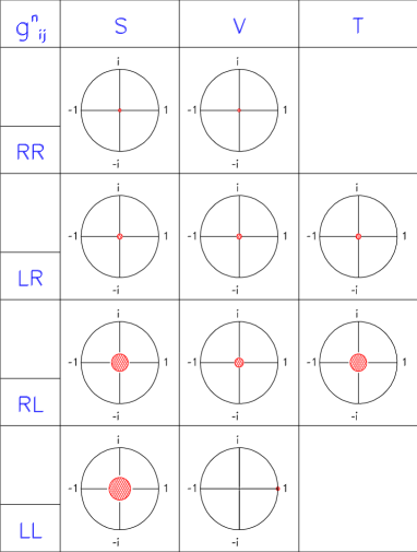
Figure 5: 90% CL experimental limits (shaded regions) [14] for the normalized $\mu$–decay couplings $g^{\prime n}_{\epsilon\omega}\equiv g^{n}_{\epsilon\omega}/N^{n}$.

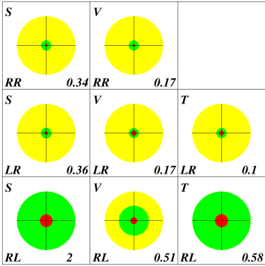
Figure 6: 90% CL experimental limits [24] for the normalized $\tau$–decay couplings $g^{\prime n}_{\epsilon\omega}\equiv g^{n}_{\epsilon\omega}/N^{n}$, assuming $e/\mu$ universality. For comparison, the $\mu$–decay limits are also shown (darker circles).

The couplings $g^{n}_{\epsilon\omega}$ can be investigated through the measurement of the final charged–lepton distribution and with the inverse decay $\nu_{l^{\prime}}l\to l^{\prime}\nu_{l}$. For $\mu$ decay, where precise measurements of the polarizations of both $\mu$ and $e$ have been performed, there exist [14] stringent bounds on the couplings involving right–handed helicities. These limits show nicely that the $\mu$–decay transition amplitude is indeed of the predicted V$-$A type: $|g^{V}_{LL}|>0.96$ (90% CL).

Figure 6 shows the most recent limits on the $\tau$ couplings [24]. The circles of unit area indicate the range allowed by the normalization constraint (14). The present experimental bounds are shown as shaded circles. For comparison, the (stronger) $\mu$-decay limits are also given (darker circles). The measurement of the $\tau$ polarization allows to bound those couplings involving an initial right–handed lepton; however, information on the final charged–lepton polarization is still lacking. The measurement of the inverse decay $\nu_{\tau}l\to\tau\nu_{l}$, needed to separate the $g^{S}_{LL}$ and $g^{V}_{LL}$ couplings, looks far out of reach.

4 NEUTRAL–CURRENT COUPLINGS

In the SM, all fermions with equal electric charge have identical vector, $v_{f}=T_{3}^{f}(1-4|Q_{f}|\sin^{2}{\theta_{W}})$ and axial–vector, $a_{f}=T_{3}^{f}$, couplings to the $Z$ boson. These neutral current couplings have been precisely tested at LEP and SLC.

The gauge sector of the SM is fully described in terms of only four parameters: $g$, $g^{\prime}$, and the two constants characterizing the scalar potential. We can trade these parameters by [1, 25, 26] $\alpha$, $G_{F}$,

$$M_{Z}=(91.1871\pm 0.0021)\,\mbox{\rm GeV}\,,$$ (15)

and $m_{H}$; this has the advantage of using the 3 most precise experimental determinations to fix the interaction. The relations

$$M_{W}^{2}s_{W}^{2}={\pi\alpha\over\sqrt{2}G_{F}}\,,\qquad\quad s_{W}^{2}=1-{M_{W}^{2}\over M_{Z}^{2}}\,,$$ (16)

determine then $s_{W}^{2}\equiv\sin^{2}{\theta_{W}}=0.2122$ and $M_{W}=80.94$ GeV; in reasonable agreement with the measured $W$ mass [25, 26], $M_{W}=80.394\pm 0.042$ GeV.

At tree level, the partial decay widths of the $Z$ boson are given by

$$\Gamma\left[Z\to\bar{f}f\right]={G_{F}M_{Z}^{3}\over 6\pi\sqrt{2}}\,\left(|v_{f}|^{2}+|a_{f}|^{2}\right)\,N_{f}\,,$$ (17)

where $N_{l}=1$ and $N_{q}=N_{C}$. Summing over all possible final fermion pairs, one predicts the total width $\Gamma_{Z}=2.474$ GeV, to be compared with the experimental value [25, 26] $\Gamma_{Z}=(2.4944\pm 0.0024)$ GeV. The leptonic decay widths of the $Z$ are predicted to be $\Gamma_{l}\equiv\Gamma(Z\to l^{+}l^{-})=84.84$ MeV, in agreement with the measured value $\Gamma_{l}=(83.96\pm 0.09)$ MeV.

Other interesting quantities are the ratios $R_{l}\equiv\Gamma(Z\to\mbox{\rm hadrons})/\Gamma_{l}$ and $R_{Q}\equiv\Gamma(Z\to\bar{Q}Q)/\Gamma(Z\to\mbox{\rm hadrons})$. The comparison between the tree–level theoretical predictions and the experimental values, shown in Table 4, is quite good.

Additional information can be obtained from the study of the fermion–pair production process $e^{+}e^{-}\to\gamma,Z\to\bar{f}f$. LEP has provided accurate measurements of the total cross-section, the forward–backward asymmetry, the polarization asymmetry and the forward–backward polarization asymmetry, at the $Z$ peak ($s=M_{Z}^{2}$):

$$\sigma^{0,f}={12\pi\over M_{Z}^{2}}\,{\Gamma_{e}\Gamma_{f}\over\Gamma_{Z}^{2}}\,, \quad{\cal A}_{\mbox{\rm\scriptsize FB}}^{0,f}={3\over 4}{\cal P}_{e}{\cal P}_{f}\,,$$

$${\cal A}_{\mbox{\rm\scriptsize Pol}}^{0,f}={\cal P}_{f}\,,\qquad\quad \quad{\cal A}_{\mbox{\rm\scriptsize FB,Pol}}^{0,f}={3\over 4}{\cal P}_{e}\,,\quad\quad$$ (18)

where $\Gamma_{f}$ is the $Z$ partial decay width to the $\bar{f}f$ final state, and

$${\cal P}_{f}\,\equiv\,{-2v_{f}a_{f}\over v_{f}^{2}+a_{f}^{2}}$$ (19)

is the average longitudinal polarization of the fermion $f$.

The measurement of the final polarization asymmetries can (only) be done for $f=\tau$, because the spin polarization of the $\tau$’s is reflected in the distorted distribution of their decay products. Therefore, ${\cal P}_{\tau}$ and ${\cal P}_{e}$ can be determined from a measurement of the spectrum of the final charged particles in the decay of one $\tau$, or by studying the correlated distributions between the final products of both $\tau^{\prime}s$ [27].

With polarized $e^{+}e^{-}$ beams, one can also study the left–right asymmetry between the cross-sections for initial left– and right–handed electrons. At the $Z$ peak, this asymmetry directly measures the average initial lepton polarization, ${\cal P}_{e}$, without any need for final particle identification. SLD has also measured the left–right forward–backward asymmetries, which are only sensitive to the final state couplings:

$${\cal A}_{\mbox{\rm\scriptsize LR}}^{0}=-{\cal P}_{e}\,,\qquad{\cal A}_{\mbox{\rm\scriptsize FB,LR}}^{0,f}=-{3\over 4}{\cal P}_{f}\,.$$ (20)

Table 4: Comparison between SM predictions and experimental [25, 26] measurements. The third column includes the main QED and QCD corrections. The experimental value for $s_{W}^{2}$ refers to the effective electroweak mixing angle in the charged–lepton sector.

Parameter	Tree–level prediction		SM fit	Experimental	Pull
	Naive	Improved	(1–loop)	value	$\left(x_{\mbox{\rm\scriptsize Exp}}-x_{\mbox{\rm\scriptsize fit}}\right)/\sigma_{\mbox{\rm\scriptsize Exp}}$
$M_{W}$   (GeV)	80.94	79.96	$80.385$	$80.394\pm 0.042$	$0.21$
$s_{W}^{2}$	0.2122	0.2311	$0.23150$	$0.23153\pm 0.00017$	$0.18$
$\Gamma_{Z}$   (GeV)	2.474	2.490	$2.4957$	$2.4944\pm 0.0024$	$-0.56$
$R_{l}$	20.29	20.88	20.740	$20.768\pm 0.024$	$1.16$
$\sigma^{0}_{\mbox{\rm\scriptsize had}}$    (nb)	42.13	41.38	41.479	$41.544\pm 0.037$	$1.75$
${\cal A}_{\mbox{\rm\scriptsize FB}}^{0,l}$	0.0657	0.0169	0.01625	$0.01701\pm 0.00095$	$0.80$
${\cal P}_{l}$	$-0.296$	$-0.150$	$-0.1472$	$-0.1497\pm 0.0016$	$-1.56$
${\cal A}_{\mbox{\rm\scriptsize FB}}^{0,b}$	0.210	0.105	0.1032	$0.0988\pm 0.0020$	$-2.20$
${\cal A}_{\mbox{\rm\scriptsize FB}}^{0,c}$	0.162	0.075	0.0738	$0.0692\pm 0.0037$	$-1.23$
${\cal P}_{b}$	$-0.947$	$-0.936$	$-0.935$	$-0.905\pm 0.026$	$1.15$
${\cal P}_{c}$	$-0.731$	$-0.669$	$-0.668$	$-0.634\pm 0.027$	$1.26$
$R_{b}$	0.219	0.220	0.21583	$0.21642\pm 0.00073$	$0.81$
$R_{c}$	0.172	0.170	0.1722	$0.1674\pm 0.0038$	$-1.27$

Using $s_{W}^{2}=0.2122$, one gets the (tree–level) predictions shown in the second column of Table 4. The comparison with the experimental measurements looks reasonable for the total hadronic cross-section $\sigma^{0}_{\mbox{\rm\scriptsize had}}\equiv\sum_{q}\,\sigma^{0,q}$; however, all leptonic asymmetries disagree with the measured values by several standard deviations. As shown in the table, the same happens with the heavy–flavour forward–backward asymmetries ${\cal A}_{\mbox{\rm\scriptsize FB}}^{0,b/c}$, which compare very badly with the experimental measurements; the agreement is however better for ${\cal P}_{b/c}$.

Clearly, the problem with the asymmetries is their high sensitivity to the input value of $\sin^{2}{\theta_{W}}$; specially the ones involving the leptonic vector coupling $v_{l}=(1-4\sin^{2}{\theta_{W}})/2$. Therefore, they are an extremely good window into higher–order electroweak corrections.

4.1 Important QED and QCD Corrections

The photon propagator gets vacuum polarization corrections, induced by virtual fermion–antifermion pairs. Their effect can be taken into account through a redefinition of the QED coupling, which depends on the energy scale of the process; the resulting effective coupling $\alpha(s)$ is called the QED running coupling. The fine structure constant is measured at very low energies; it corresponds to $\alpha(m_{e}^{2})$. However, at the $Z$ peak, we should rather use $\alpha(M_{Z}^{2})$. The long running from $m_{e}$ to $M_{Z}$ gives rise to a sizeable correction [13, 28]: $\alpha(M_{Z}^{2})^{-1}=128.878\pm 0.090\,$. The quoted uncertainty arises from the light–quark contribution, which is estimated from $\sigma(e^{+}e^{-}\to\mbox{\rm hadrons})$ and $\tau$–decay data.

Since $G_{F}$ is measured at low energies, while $M_{W}$ is a high–energy parameter, the relation between both quantities in Eq. (16) is clearly modified by vacuum–polarization contributions. One gets then the corrected predictions $M_{W}=79.96$ GeV and $s^{2}_{W}=0.2311$.

The gluonic corrections to the $Z\to\bar{q}q$ decays can be directly incorporated by taking an effective number of colours $N_{q}=N_{C}\,\left\{1+{\alpha_{s}\over\pi}+\ldots\right\}\,\approx\,3.12$, where we have used $\alpha_{s}(M_{Z}^{2})\approx 0.12\,$.

The third column in Table 4 shows the numerical impact of these QED and QCD corrections. In all cases, the comparison with the data gets improved. However, it is in the asymmetries where the effect gets more spectacular. Owing to the high sensitivity to $s^{2}_{W}$, the small change in the value of the weak mixing angle generates a huge difference of about a factor of 2 in the predicted asymmetries. The agreement with the experimental values is now very good.

4.2 Higher–Order Electroweak Corrections

Initial– and final–state photon radiation is by far the most important numerical correction. One has in addition the contributions coming from photon exchange between the fermionic lines. All these QED corrections are to a large extent dependent on the detector and the experimental cuts, because of the infra-red problems associated with massless photons. (one needs to define, for instance, the minimun photon energy which can be detected). These effects are usually estimated with Monte Carlo programs and subtracted from the data.

More interesting are the so–called oblique corrections, gauge–boson self-energies induced by vacuum polarization diagrams, which are universal (process independent). In the case of the $W^{\pm}$ and the $Z$, these corrections are sensitive to heavy particles (such as the top) running along the loop [29]. In QED, the vacuum polarization contribution of a heavy fermion pair is suppressed by inverse powers of the fermion mass. At low energies ($s<<m_{f}^{2}$), the information on the heavy fermions is then lost. This decoupling of the heavy fields happens in theories like QED and QCD, with only vector couplings and an exact gauge symmetry [30]. The SM involves, however, a broken chiral gauge symmetry. The $W^{\pm}$ and $Z$ self-energies induced by a heavy top generate contributions which increase quadratically with the top mass [29]. The leading $m_{t}^{2}$ contribution to the $W^{\pm}$ propagator amounts to a $-3\%$ correction to the relation (16) between $G_{F}$ and $M_{W}$.

Owing to an accidental $SU(2)_{C}$ symmetry of the scalar sector, the virtual production of Higgs particles does not generate any $m_{H}^{2}$ dependence at one loop [29]. The dependence on the Higgs mass is only logarithmic. The numerical size of the correction induced on (16) is $-0.3\%$ ($+1\%$) for $m_{H}=60$ (1000) GeV.

Figure 7: $m_{t}$–dependent corrections to the $Z\bar{b}b$ vertex.

The vertex corrections are non-universal and usually smaller than the oblique contributions. There is one interesting exception, the $Z\bar{b}b$ vertex, which is sensitive to the top quark mass [31]. The $Z\bar{f}f$ vertex gets 1–loop corrections where a virtual $W^{\pm}$ is exchanged between the two fermionic legs. Since, the $W^{\pm}$ coupling changes the fermion flavour, the decays $Z\to\bar{d}_{i}\bar{d}_{i}$ get contributions with a top quark in the internal fermionic lines. These amplitudes are suppressed by a small quark–mixing factor $|V_{td_{i}}|^{2}$, except for the $Z\to\bar{b}b$ vertex because $|V_{tb}|\approx 1$. The explicit calculation [31, 32] shows the presence of hard $m_{t}^{2}$ corrections to the $Z\to\bar{b}b$ vertex, which amount to a $-1.5\%$ effect in $\Gamma(Z\to\bar{b}b)$.

The non-decoupling present in the $Z\bar{b}b$ vertex is quite different from the one happening in the boson self-energies. The vertex correction does not have any dependence with the Higgs mass. Moreover, while any kind of new heavy particle, coupling to the gauge bosons, would contribute to the $W^{\pm}$ and $Z$ self-energies, possible new–physics contributions to the $Z\bar{b}b$ vertex are much more restricted and, in any case, different. Therefore, an independent experimental test of the two effects is very valuable in order to disentangle possible new–physics contributions from the SM corrections.

The remaining quantum corrections (box diagrams, Higgs exchange) are rather small at the $Z$ peak.

4.3 Lepton Universality

Table 5: Measured values [25, 26] of $\Gamma_{l}$ and the leptonic forward–backward asymmetries. The last row shows the combined result (for a massless lepton) assuming lepton universality.

	$\Gamma_{l}$   (MeV)	${\cal A}_{\mbox{\rm\scriptsize FB}}^{0,l}$   (%)
$e$	$83.90\pm 0.12$	$1.45\pm 0.24$
$\mu$	$83.96\pm 0.18$	$1.67\pm 0.13$
$\tau$	$84.05\pm 0.22$	$1.88\pm 0.17$
$l$	$83.96\pm 0.09$	$1.701\pm 0.095$

Table 6: Measured values [25, 26] of the leptonic polarization asymmetries.

$-{\cal A}_{\mbox{\rm\scriptsize Pol}}^{0,\tau}=-{\cal P}_{\tau}$	$0.1425\pm 0.0044$
$-{4\over 3}{\cal A}^{0,\tau}_{\mbox{\rm\scriptsize FB,Pol}}=-{\cal P}_{e}$	$0.1483\pm 0.0051$
${\cal A}_{\mbox{\rm\scriptsize LR}}^{0}=-{\cal P}_{e}$	$0.1511\pm 0.0022$
$\!\{{4\over 3}{\cal A}_{\mbox{\rm\scriptsize FB}}^{0,l}\}^{1/2}=-P_{l}\!$	$0.1506\pm 0.0042$
${4\over 3}{\cal A}^{0,e}_{\mbox{\rm\scriptsize FB,LR}}\Rightarrow-{\cal P}_{e}$	$0.1558\pm 0.0064$
${4\over 3}{\cal A}^{0,\mu}_{\mbox{\rm\scriptsize FB,LR}}=-{\cal P}_{\mu}$	$0.137\pm 0.016$
${4\over 3}{\cal A}^{0,\tau}_{\mbox{\rm\scriptsize FB,LR}}=-{\cal P}_{\tau}$	$0.142\pm 0.016$

Figure 8: 68% probability contours in the $a_{l}$-$v_{l}$ plane from LEP measurements [25]. The solid contour assumes lepton universality. Also shown is the $1\sigma$ band resulting from the ${\cal A}_{\mbox{\rm\scriptsize LR}}^{0}$ measurement at SLD. The shaded region corresponds to the SM prediction for $m_{t}=174.3\pm 5.1$ GeV and $m_{H}=300^{+700}_{-210}$ GeV. The arrows point in the direction of increasing $m_{t}$ and $m_{H}$ values.

Tables 6 and 6 show the present experimental results for the leptonic $Z$ decay widths and asymmetries. The data are in excellent agreement with the SM predictions and confirm the universality of the leptonic neutral couplings. The average of the two $\tau$ polarization measurements, ${\cal A}_{\mbox{\rm\scriptsize Pol}}^{0,\tau}$ and ${4\over 3}{\cal A}^{0,\tau}_{\mbox{\rm\scriptsize FB,Pol}}$, results in ${\cal P}_{l}=-0.1450\pm 0.0033$ which deviates by $1.5\,\sigma$ from the ${\cal A}^{0}_{LR}$ measurement. Assuming lepton universality, the combined result from all leptonic asymmetries gives

$${\cal P}_{l}=-0.1497\pm 0.0016\,.$$ (21)

Figure 8 shows the 68% probability contours in the $a_{l}$–$v_{l}$ plane, obtained from a combined analysis [25] of all leptonic observables. Lepton universality is now tested to the $0.15\%$ level for the axial–vector neutral couplings, while only a few per cent precision has been achieved for the vector couplings [26]:

$${a_{\mu}\over a_{e}}=1.0001\pm 0.0014 {v_{\mu}\over v_{e}}=0.981\pm 0.082\,,$$ ,

$${a_{\tau}\over a_{e}}=1.0019\pm 0.0015 {v_{\tau}\over v_{e}}=0.964\pm 0.032\,.$$ ,

The neutrino couplings can be determined from the invisible $Z$–decay width, $\Gamma_{\mbox{\rm\scriptsize inv}}/\Gamma_{l}=5.941\pm 0.016$, by assuming three identical neutrino generations with left–handed couplings and fixing the sign from neutrino scattering data [33]. The resulting experimental value [25], $v_{\nu}=a_{\nu}=0.50123\pm 0.00095$, is in perfect agreement with the SM. Alternatively, one can use the SM prediction, $\Gamma_{\mbox{\rm\scriptsize inv}}/\Gamma_{l}=(1.9912\pm 0.0012)\,N_{\nu}$, to get a determination of the number of (light) neutrino flavours [25, 26]:

$$N_{\nu}=2.9835\pm 0.0083\,.$$ (22)

The universality of the neutrino couplings has been tested with $\nu_{\mu}e$ scattering data, which fixes [34] the $\nu_{\mu}$ coupling to the $Z$:  $v_{\nu_{\mu}}=a_{\nu_{\mu}}=0.502\pm 0.017$.

Assuming lepton universality, the measured leptonic asymmetries can be used to obtain the effective electroweak mixing angle in the charged–lepton sector ($\chi^{2}/\mbox{d.o.f.}=3.4/4$):

$$\sin^{2}{\theta^{\mbox{\rm\scriptsize lept}}_{\mbox{\rm\scriptsize eff}}}\equiv{1\over 4}\left(1-{v_{l}\over a_{l}}\right)\,=\,0.23119\pm 0.00021\,.$$

Including also the information provided by the hadronic asymmetries, one gets [25, 26] $\sin^{2}{\theta^{\mbox{\rm\scriptsize lept}}_{\mbox{\rm\scriptsize eff}}}=0.23153\pm 0.00017$, with a $\chi^{2}/\mbox{d.o.f.}=13.3/7$.

4.4 SM Electroweak Fit

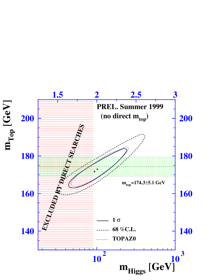
Figure 9: Contours in $m_{t}$ and $m_{H}$ obtained from the SM electroweak fit. Also shown are the 95% exclusion limit on $m_{H}$ from direct searches and the Fermilab measurement of $m_{t}$ [25].

The high accuracy of the present data provides compelling evidence for the pure weak quantum corrections, beyond the main QED and QCD corrections discussed in Section 4.1. The measurements are sufficiently precise to require the presence of quantum corrections associated with the virtual exchange of top quarks, gauge bosons and Higgses.

Figure 9 shows the constraints obtained on $m_{t}$ and $m_{H}$, from a global fit to the electroweak data [25]. The fitted value of the top mass is in excellent agreement with the direct Tevatron measurement $m_{t}=174.3\pm 5.1$ GeV [25]. The data prefers a light Higgs, close to the present lower bound from direct searches, $m_{H}>95.2$ GeV (95% CL). There is a large correlation between the fitted values of $m_{t}$ and $m_{H}$; the correlation would be much larger if the $R_{b}$ measurement was not used ($R_{b}$ is insensitive to $m_{H}$). The fit gives the upper bound [25]:

$$m_{H}<245\;\mbox{\rm GeV}\qquad(95\%\,\mbox{\rm CL})\,.$$ (23)

The global fit results in an extracted value of the strong coupling, $\alpha_{s}(M_{Z}^{2})=0.119\pm 0.003$, which agrees very well with the world average value [14] $\alpha_{s}(M_{Z}^{2})=0.119\pm 0.002$.

As shown in Table 4, the different electroweak measurements are well reproduced by the SM electroweak fit. At present, the larger deviation appears in ${\cal A}_{\mbox{\rm\scriptsize FB}}^{0,b}$, which seems to be too low by $2.2\,\sigma$.

The uncertainty on the QED coupling $\alpha(M_{Z}^{2})^{-1}$ introduces a severe limitation on the accuracy of the SM predictions. The uncertainty of the “standard” value, $\alpha(M_{Z}^{2})^{-1}=128.878\pm 0.090$ [28], causes an error of $0.00023$ on the $\sin^{2}{\theta^{\mbox{\rm\scriptsize lept}}_{\mbox{\rm\scriptsize eff}}}$ prediction. A recent analysis [13], using hadronic $\tau$–decay data, results in a more precise value, $\alpha(M_{Z}^{2})^{-1}=128.933\pm 0.021$, reducing the corresponding uncertainty on $\sin^{2}{\theta^{\mbox{\rm\scriptsize lept}}_{\mbox{\rm\scriptsize eff}}}$ to $5\times 10^{-4}$; this translates into a $30\%$ reduction in the error of the fitted $\log{\left(m_{H}\right)}$ value.

To improve the present determination of $\alpha(M_{Z}^{2})^{-1}$ one needs to perform a good measurement of $\sigma(e^{+}e^{-}\to\mbox{\rm hadrons})$, as a function of the centre–of–mass energy, in the whole kinematical range spanned by DA$\Phi$NE, a tau–charm factory and the B factories. This would result in a much stronger constraint on the Higgs mass.

5 SUMMARY

The SM provides a beautiful theoretical framework which is able to accommodate all our present knowledge on electroweak interactions. It is able to explain any single experimental fact and, in some cases, it has successfully passed very precise tests at the 0.1% to 1% level. However, there are still pieces of the SM Lagrangian which so far have not been experimentally analyzed in any precise way.

The gauge self-couplings are presently being investigated at LEP2, through the study of the $e^{+}e^{-}\to W^{+}W^{-}$ production cross-section. The $V-A$ ($\nu_{e}$-exchange in the $t$ channel) contribution generates an unphysical growing of the cross-section with the centre-of-mass energy, which is compensated through a delicate gauge cancellation with the $e^{+}e^{-}\to\gamma,Z\to W^{+}W^{-}$ amplitudes. The recent LEP2 measurements of $\sigma(e^{+}e^{-}\to W^{+}W^{-})$, in good agreement with the SM, have provided already convincing evidence [25] for the contribution coming from the $ZWW$ vertex.

The study of this process has also provided a more accurate measurement of $M_{W}$, allowing to improve the precision of the neutral–current analyses. The present LEP2 determination, $M_{W}=80.350\pm 0.056$ GeV, is already more precise than the value $M_{W}=80.448\pm 0.062$ GeV obtained in $p\bar{p}$ colliders. Moreover it is in nice agreement with the result $M_{W}=80.364\pm 0.029$ GeV obtained from the indirect SM fit of electroweak data [25].

The Higgs particle is the main missing block of the SM framework. The data provide a clear confirmation of the assumed pattern of spontaneous symmetry breaking, but do not prove the minimal Higgs mechanism embedded in the SM. At present, a relatively light Higgs is preferred by the indirect precision tests. LHC will try to find out whether such scalar field exists.

In spite of its enormous phenomenological success, the SM leaves too many unanswered questions to be considered as a complete description of the fundamental forces. We do not understand yet why fermions are replicated in three (and only three) nearly identical copies? Why the pattern of masses and mixings is what it is? Are the masses the only difference among the three families? What is the origin of the SM flavour structure? Which dynamics is responsible for the observed CP violation?

Clearly, we need more experiments in order to learn what kind of physics exists beyond the present SM frontiers. We have, fortunately, a very promising and exciting future ahead of us.

This work has been supported in part by the ECC, TMR Network $EURODAPHNE$ (ERBFMX-CT98-0169), and by DGESIC (Spain) under grant No. PB97-1261.

References

- [1] A. Pich, The Standard Model of Electroweak Interactions, Proc. XXII International Winter Meeting on Fundamental Physics: The Standard Model and Beyond (Jaca, 1994) eds. J.A. Villar and A. Morales (Editions Frontières, Gif-sur-Yvette, 1995), p. 1 [hep-ph/9412274].
- [2] A. Pich, Quantum Chromodynamics, Proc. 1994 European School of High Energy Physics (Sorrento, 1994), eds. N. Ellis and M.B. Gavela, Report CERN 95-04 (Geneva, 1995), p. 157 [hep-ph/9505231].
- [3] T. Kinoshita (editor), Quantum Electrodynamics, Advanced Series on Directions in High Energy Physics, Vol. 7 (World Scientific, Singapore, 1990).
- [4] T. Kinoshita, Rep. Prog. Phys. 59 (1996) 1459.
- [5] A. Czarnecki and W.J. Marciano, Lepton anomalous magnetic moments – a theory update, in [35] 245; A. Czarnecki, B. Krause and W.J. Marciano, Phys. Rev. Lett. 76 (1996) 3267; Phys. Rev. D52 (1995) 2619.
- [6] S. Peris, M. Perrotet and E. de Rafael, Phys. Lett. B355 (1995) 523.
- [7] T.V. Kukhto et al, Nucl. Phys. B371 (1992) 567.
- [8] B. Krause, Phys. Lett. B390 (1997) 392.
- [9] S. Laporta and E. Remiddi, Phys. Lett. B379 (1996) 283.
- [10] E. de Rafael, Phys. Lett. B322 (1994) 239.
- [11] M. Hayakawa and T. Kinoshita, Phys. Rev. D57 (1998) 465; M. Hayakawa, T. Kinoshita and A.I. Sanda, Phys. Rev. D54 (1996) 3137; T. Kinoshita and A.I. Sanda, Phys. Rev. Lett. 75 (1995) 790.
- [12] J. Bijnens, E. Pallante and J. Prades, Nucl. Phys. B474 (1996) 379; Phys. Rev. Lett. 75 (1995) 1447, 3781.
- [13] M. Davier, Evaluation of and , in [35] 327; R. Alemany, M. Davier and A. Höcker, Eur. Phys. J. C2 (1998) 123; M. Davier and A. Höcker, Phys. Lett. B419 (1998) 419.
- [14] Particle Data Group, Review of Particle Physics, Eur. Phys. J. C3 (1998) 1; and 1999 off-year partial update for the 2000 edition [http://pdg.lbl.gov/].
- [15] The Second DANE Physics Handbook, eds. L. Maiani, G. Panchieri and N. Paver (Frascati, 1995).
- [16] M. Grosse Perdekamp et al (BNL-E821), Status of the experiment at BNL, in [35] 253.
- [17] T. Kinoshita and A. Sirlin, Phys. Rev. 113 (1959) 1652; W.J. Marciano and A. Sirlin, Phys. Rev. Lett. 61 (1988) 1815.
- [18] T. van Ritbergen and R.G. Stuart, Phys. Rev. Lett. 82 (1999) 488; hep-ph/9904240; P. Malde and R.G. Stuart, Nucl. Phys.B552 (1999) 41.
- [19] A. Pich, Tau Physics, talk at the 1999 Lepton–Photon Conference (Stanford, August 1999); Tau Lepton Physics: Theory Overview, Proc. Fourth Workshop on Tau Lepton Physics –TAU96– (Colorado, 16–19 September 1996), ed. J. Smith, Nucl. Phys. B (Proc. Suppl.) 55C (1997) 3.
- [20] L. Michel, Proc. Phys. Soc. A63 (1950) 514; 1371; C. Bouchiat and L. Michel, Phys. Rev. 106 (1957) 170.
- [21] T. Kinoshita and A. Sirlin, Phys. Rev. 107 (1957) 593; 108 (1957) 844.
- [22] W. Fetscher et al, Phys. Lett. B173 (1986) 102.
- [23] A. Pich and J.P. Silva, Phys. Rev. D52 (1995) 4006.
- [24] I. Boyko, Tests of lepton universality in tau decays, talk at EPS-HEP99 (Tampere, July 1999).
- [25] The LEP Collaborations ALEPH, DELPHI, L3, OPAL, the LEP Electroweak Working Group and the SLD Heavy Flavour and Electroweak Groups, A Combination of Preliminary Electroweak Measurements and Constraints on the Standard Model, CERN-EP/99-15 (February 1999); and summer update [http://www.cern.ch/LEPEWWG/].
- [26] M. Swartz, Precision Electroweak Physics at the Z, talk at the 1999 Lepton–Photon Conference (Stanford, August 1999).
- [27] R. Alemany et al, Nucl. Phys. B379 (1992) 3; M. Davier et al, Phys. Lett. B306 (1993) 411.
- [28] S. Eidelmann and F. Jegerlehner, Z. Phys. C67 (1995) 585.
- [29] M. Veltman, Nucl. Phys. B123 (1977) 89.
- [30] T. Appelquist and J. Carazzone, Phys. Rev. D11 (1975) 2856.
- [31] J. Bernabéu, A. Pich and A. Santamaría, Phys. Lett. B200 (1988) 569; Nucl. Phys. B363 (1991) 326.
- [32] A.A. Akhundov et al, Nucl. Phys. B276 (1986) 1; W. Beenakker and W. Hollik, Z. Phys. C40 (1988) 141; B.W. Lynn and R.G. Stuart, Phys. Lett. B252 (1990) 676.
- [33] P. Vilain et al (CHARM II), Phys. Lett. B335 (1994) 246.
- [34] P. Vilain et al (CHARM II), Phys. Lett. B320 (1994) 203.
- [35] A. Pich and A Ruiz (editors), Proc. Fifth Workshop on Tau Lepton Physics –TAU’98– (Santander, 16–19 September 1998), Nucl. Phys. B (Proc. Suppl.) 76 (1999).