Dynamics of Nontopological Solitons - Q Balls

Abstract

We use numerical simulations and semi-analytical methods to investigate the stability and the interactions of nontopological stationary qball solutions. In the context of a simple model we map the parameter sectors of stability for a single qball and verify the result using numerical simulations of time evolution. The system of two interacting qballs is also studied in one and two space dimensions. We find that the system generically performs breather type oscillations with frequency equal to the difference of the internal qball frequencies. This result is shown to be consistent with the form of the qball interaction potential. Finally we perform simulations of qball scattering and show that the right angle scattering effect observed in topological soliton scattering in two dimensions, persists also in the case of qballs where no topologically conserved quantities are present. For relativistic collision velocities the qball charge is split into a forward and a right angle scattering component. As the collision velocity increases, the forward component gets amplified at the expense of the right angle component.

I Introduction

It is well known that realistic supersymmetric theories are associated with a number of scalar fields with various charges. These theories and in particular the MSSM allow for baryonic and leptonic nontopological solitons[1] known as qballs[2]. They are composed of squarks, sleptons and Higgs scalars [3, 4] and they originate through the breakup of an Affleck-Dine condensate carrying a net baryon and/or lepton number[5]. Such objects could have interesting cosmological consequences. For example they could be responsible for both the net baryon number of the universe and its dark matter component[4].

The basic properties of qballs have been studied extensively in the literature using mainly analytical and semi-analytical methods[1]. These methods are particularly useful in understanding basic properties of qballs like existence, small vibrations, stability in certain parameter limits (thick[3] or thin wall[2] approximation) but they can not be very illuminating in understanding more complicated issues like scattering, interactions or stability for arbitrary parameters. The goal of this paper is to use numerical simulations of qball evolution in one and two spatial dimensions, along with semi-analytical methods in order to study the stability under small fluctuations, the interactions and the scattering of qballs.

The structure of the paper is the following: In the next section we introduce a simple model and show the existence of stable qball solutions in its context. By considering small fluctuations superposed on these solutions for various parameters we construct a map showing the stability sectors in parameter space. These sectors are then verified by performing numerical simulations of time evolution for the solutions considered. A virial theorem is also derived and its validity is demonstrated numerically. In section III we consider a system of two interacting qballs and show analytically that the interaction potential is time dependent and periodic. This type of interaction is verified by performing numerical simulations of qball evolution which shows that the system performs breather-type oscillations with the analytically predicted frequency. In section IV we use boosted qball configurations to perform scattering numerical experiments in 2+1 dimensions showing that for low collision velocities qballs tend to scatter at right angles like their topological counterparts. For relativistic collision velocities we find that the qball charge splits into a forward and a right angle component. The forward component gets amplified as the velocity increases. Finally in section V we conclude, summarize and briefly discuss future extensions of this work.

II Stability - Virial Theorem

Consider a complex scalar field $\Phi$ in 1+1 dimensions whose dynamics is determined by the Lagrangian

$${\cal L}={1\over 2}\partial_{\mu}\Phi^{*}\partial^{\mu}\Phi-U(\Phi),$$ (1)

where

$$U(\Phi)={1\over 2}m^{2}|\Phi|^{2}-{1\over 3}\alpha|\Phi|^{3}+{1\over 4}b|\Phi|^{4}.$$ (2)

Using a rescaling

$$\Phi \rightarrow {m^{2}\over\alpha}\Phi,$$ (3)

$$x \rightarrow {x\over m},$$ (4)

the Lagrangian (1) gets simplified as follows

$${\cal L}={1\over 2}\partial_{\mu}\Phi^{*}\partial^{\mu}\Phi-{1\over 2}|\Phi|^{2}+{1\over 3}|\Phi|^{3}-{1\over 4}B|\Phi|^{4},$$ (5)

where

$$B\equiv{{bm^{2}}\over\alpha^{2}}.$$ (6)

This leads to the field equation

$${\ddot{\Phi}}-\Phi^{\prime\prime}+\Phi-|\Phi|\Phi+B|\Phi|^{2}\Phi=0.$$ (7)

Using the usual qball ansatz

$$\Phi(x)=\sigma(x)e^{i\omega t}$$ (8)

with the conserved Noether charge

$$Q = {1\over 2i}\int_{-\infty}^{+\infty}dx\;(\Phi^{*}\,\partial_{t}\Phi-\Phi\,\partial_{t}\Phi^{*})$$ (9)

$$= \omega\int_{-\infty}^{+\infty}dx\;\sigma(x)^{2}$$ (10)

we obtain the field equation for $\sigma(x)$

$$\sigma^{\prime\prime}+(\omega^{2}-1)\sigma+\sigma^{2}-B\sigma^{3}=0.$$ (11)

The requirement of finite energy and the asymptotics obtained from equation (11) imply the boundary conditions

$$\sigma^{\prime}(0) = 0,$$ (12)

$$\sigma(\infty) = 0.$$ (13)

The combination of equations (11) and (11-12) are identical to the dynamical equations describing the motion of a virtual particle that starts at rest at ‘time’ $x=0$ from some position $\sigma_{0}$ and moves to $\sigma=0$ at ‘time’ $x\rightarrow\infty$ under the influence of the effective potential

$$V_{eff}={1\over 2}(\omega^{2}-1)|\Phi|^{2}+{1\over 3}|\Phi|^{3}-{1\over 4}B|\Phi|^{4}$$ (14)

.

By considering the form of the effective potential (14) it becomes clear that in order to have a solution with the boundary conditions (11-12) the following conditions must be satisfied

• Symmetry must be broken by the effective potential (14) ($m_{eff}^{2}\equiv\omega^{2}-1<0$)

• There must be at least one intersection point of $V_{eff}(\sigma)$ with the $V_{eff}(|\Phi|)=0$ axis.

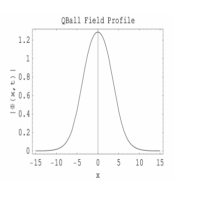
FIG. 1.: The field magnitude profile $|\Phi(x,t)|$ of a qball solution for $B=4/9$, $\omega^{2}=0.51$.

The first condition implies $\omega^{2}<1$ while the second condition implies that the equation $V_{eff}=0$ has at least one real solution different from 0. It is easy to show that the constraints imposed on $\omega$ by these two conditions can be written as

$$1-{2\over{9B}}<\omega^{2}<1.$$ (15)

The energy density of the system (1) is

$${\cal E}=|{\dot{\Phi}}|^{2}+|\Phi^{\prime}|^{2}+|\Phi|^{2}-{2\over 3}|\Phi|^{3}+{B\over 2}|\Phi|^{4}$$ (16)

which with the qball ansatz (8) becomes

$${\cal E}=\sigma^{\prime 2}+(1+\omega^{2})\sigma^{2}-{2\over 3}\sigma^{3}+{B\over 2}\sigma^{4}.$$ (17)

Our main goal is to study numerically the dynamics and the stability of single and multi-qball configurations in the context of the simple model (1). The first step in that direction is to solve equation (11) numerically (in a parameter region where qball solutions exist), to find the single qball profile and then evolve numerically the solution according to (7) checking total energy and charge conservation.

Fig. 1 shows the numerically obtained qball profile for $B=4/9$ and $\omega^{2}=0.51$ using a fourth order Runge-Kutta scheme. The evolution of this configuration in time when used as initial condition in equation (7) with periodic boundary conditions has been performed and found to correspond to a stable configuration. The total energy and charge Q were conserved to within about 3% during the evolution.

Static scalar field configurations in space dimensions higher than two are unstable towards collapse because both the gradient and the potential terms of the energy may be shown to decrease with a rescaling of the configuration corresponding to collapse[6]. On the other hand the stability of the stationary (time dependent) qball configuration towards collapse or expansion is a result of the different behavior of kinetic (time dependent) and potential terms towards spatial rescaling of the field configuration. This fact may be seen even in 1+1 dimensions by expressing the energy as a sum of kinetic, gradient and potential terms

$$E=I_{1}+I_{2}+I_{3},$$ (18)

where

$$I_{1} = \int_{-\infty}^{+\infty}dx\;\omega^{2}\;\sigma^{2}={Q^{2}\over{\int dx\;\sigma^{2}}},$$ (19)

$$I_{2} = \int_{-\infty}^{+\infty}dx\;\sigma^{\prime 2},$$ (20)

$$I_{3} = \int_{-\infty}^{+\infty}dx\;(\sigma^{2}-{2\over 3}\sigma^{3}+{B\over 2}\sigma^{4}).$$ (21)

After a rescaling of the spatial coordinate $x\rightarrow\alpha x$ the expression of the total energy becomes

$$E_{\alpha}={1\over\alpha}(I_{1}+I_{2})+\alpha I_{3}.$$ (22)

For stability we demand that the energy is minimized for $\alpha=1$ which implies that

$${{dE_{\alpha}}\over{d\alpha}}|_{\alpha=1}=0\Rightarrow I_{1}+I_{2}=I_{3}$$ (23)

while the second derivative is ${{d^{2}E_{\alpha}}\over{d\alpha}^{2}}|_{\alpha=1}=2\>(I_{1}+I_{2})>0$, implying energy minimum and therefore stability. Thus the stability of the qball configuration towards coordinate rescaling implies the validity of the virial theorem of equation (23) connecting the potential energy with the gradient energy and the kinetic energy (for a similar virial theorem see Ref. [3]). We have confirmed numerically the validity of the virial theorem (23) and the virial ratio ${{I_{1}+I_{2}-I_{3}}\over{I_{1}+I_{2}+I_{3}}}$ was found to be zero to within less than 1% for various values of $\omega$ where qball solutions exist and for various $B$ in the range $2/9<B<1$.

In order to study the stability of the qball configuration under small fluctuations that conserve the charge Q of equation (10) we must consider variations of the energy obtained from the density (17) and expressed in terms of Q.

$$E=\int dx\;[\sigma^{\prime 2}+\sigma^{2}-{2\over 3}\sigma^{3}+{B\over 2}\sigma^{4}]+{Q^{2}\over{\int dx\;\sigma^{2}}}.$$ (24)

Since the qball is a stationary solution of the field equations, the first variation of (24) with respect to $\sigma$ vanishes identically. The second variation may be written as

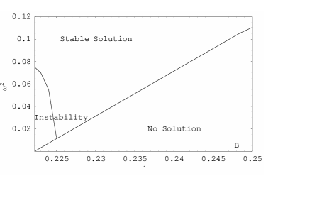
FIG. 2.: Parameter sectors of existence and stability for qball solutions.

$$\delta^{2}E=\int dx\;\delta\sigma{\hat{O}}\delta\sigma,$$ (25)

where

$${\hat{O}}=-{{d^{2}}\over{dx^{2}}}+(1-2\sigma_{0}+3B\sigma_{0}^{2})+3\omega^{2},$$ (26)

and $\sigma_{0}$ is the unperturbed qball solution. For stability we require $\delta^{2}E>0$ for all fluctuations that conserve charge. This is equivalent to demanding that the Hermitian operator ${\hat{O}}$ has no negative eigenvalues. In order to find the parameter region corresponding to stability (no negative eigenvalues) we have solved the differential equation

$${\hat{O}}\delta\sigma=0$$ (27)

with initial conditions $\delta\sigma(0)=1$ and $\delta\sigma^{\prime}(0)=0$ using a fourth order Runge-Kutta scheme. By varying the parameters $B,\;\omega$ we have identified the line in parameter space where the eigenvalue problem (27) has a ground state with zero eigenvalue. This line clearly separates the parameter sector of stability from the corresponding sector where the equation (27) has negative eigenvalues and the qball is unstable.

Fig. 2 shows part of the parameter space divided in three sectors: the sector where stable qball solutions exist, the sector where qball solutions exist but they are unstable and the sector where no qball solutions exist because the condition (15) is violated. The scale of the plot was chosen in order to magnify the sector of instability which would otherwise be too small to be seen.

We have tested and verified the validity of these sectors by simulating numerically the evolution of an isolated qball using (7) in the instability and in the stability sectors.

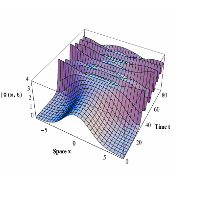
FIG. 3.: Evolution of a qball solution in the instability sector. The evolution of the field magnitude $\Phi(x,t)$ is plotted. The time evolution was performed in the range $-7.5<x<7.5$.

Fig. 3 shows an example of evolution of a qball in the instability sector. On the other hand we have also verified stability by performing the time evolution of the field amplitude for a qball in the stability sector ($\omega^{2}=0.1\;B=2/9\simeq 0.222$). The qball was seen to remain stable and evolved undistorted in time even though the evolution lasted for ten internal frequency periods ($t_{max}=10({{2\pi}\over\omega}$)). Fig. 3 shows the same numerical experiment for parameters in the instability sector ($\omega^{2}=0.05\;B=2/9\simeq 0.222$) where equation (27) has negative eigenvalues. The evolution lasted only three internal frequency periods ($t_{max}=3({{2\pi}\over\omega}$)) but the qball configuration got rapidly distorted and decayed into plane waves thus verifying the semi-analytical prediction for instability.

III Interactions - Scattering

We now consider multi-qball configurations in order to study their interactions and their scattering properties using mainly numerical simulations of evolution. For a two qball initial configuration we use the ansatz

$$\Phi(x,t)=\sigma_{+}e^{i\omega_{+}t}+\sigma_{-}e^{i\omega_{-}t}$$ (28)

where $\sigma_{+}\equiv\sigma_{1}(x+x_{0})$ and $\sigma_{-}\equiv\sigma_{2}(x-x_{0})$ with $\sigma_{1}$ ($\sigma_{2}$) the field magnitude for a single qball with $\omega=\omega_{+}$ ($\omega=\omega_{-}$).

The interaction potential between the two qballs can be obtained by subtracting the energy densities $\epsilon_{+}(x,t)$, $\epsilon_{-}(x,t)$ of each non-interacting qball from the energy density of the total interacting configuration. After a straightforward calculation we obtain the interaction energy as

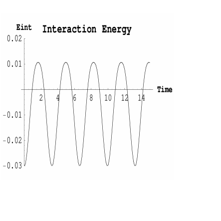
FIG. 4.: The interaction energy of a pair of qballs calculated using the expression of ${\cal E}_{int}$ with $B=4/9$, $\omega^{2}=0.9$ showing a behavior of the form $-\cos(2\omega t)$.

$${\cal E}_{int} = \sigma_{+}\sigma_{-}\cos[(\omega_{+}-\omega_{-})t]\;F(\sigma_{+},\sigma_{-},\omega_{+},\omega_{-})$$

$$+\sigma^{2}_{+}\sigma^{2}_{-}\cos^{2}[(\omega_{+}-\omega_{-})t]+G(\sigma_{+},\sigma_{-})$$

where $F$ and $G$ are time independent functions of $O(1)$ and $O(\sigma_{+}\sigma_{-})$ respectively. It is easy to see from the field equation (11) that the fields $\sigma_{\pm}$ decay exponentially at infinity and therefore the term proportional to $F$ dominates in the interaction energy. We therefore expect that the two qball system will perform oscillations with characteristic angular frequency $\omega_{+}-\omega_{-}$ while slowly drifting due to the effect of the small constant interaction term $G$. Indeed this is what we see in the numerical simulations of the time evolution of the system.

We have considered the ansatz (28) with $\omega_{+}=\omega_{int}$ and $\omega_{-}=-\omega_{int}$ which implies $\sigma_{1}(x)=\sigma_{2}(x)$ since the internal angular frequencies of field rotation are opposite. The interaction energy of this system obtained numerically for $\omega_{int}=0.9$ as described above by using the numerically calculated $\sigma(x)$, is time dependent and is shown in Fig. 4.

This interaction energy however assumes that the form of the initial ansatz is retained during the time evolution of the system and should therefore be subject to test by numerical simulation. As expected from the expression of ${\cal E}_{int}$ the time dependence of the ansatz interaction is proportional to $\cos(2\omega_{int}t)$.

In order to test if the predicted time dependence of the interaction is realized in a realistic system we have performed a numerical simulation of the evolution of the ansatz (28) by solving equation (7) using a leapfrog algorithm, periodic boundary conditions and initial conditions based on (28). The parameter values were $B=4/9$, $\omega^{2}_{int}=0.9$ and the initial qball distance was $2x_{0}=10$ in a lattice of $2d=30$ (these are dimensionless due to the rescaling of the Lagrangian). The evolution of the field magnitude $|\Phi(x,t)|$ is shown in Fig. 5 where the oscillations of the system can be seen clearly. The period and the angular frequency of these oscillations can be found by plotting the location of the field maxima as a function of time. This is shown in Fig. 6 where we plot the location $x_{max}(t)$ of the maximum of $|\Phi(x,t)|$ for $x>0$ and $0<t<15$. Clearly the location of the qball at $x>0$ described by $x_{max}(t)$ performs oscillations due to the interactions with the qball at $x<0$. The period of these oscillations can easily be seen from Fig. 6 to be approximately $T\simeq 3.5$ which is consistent with the anticipated result $T={{2\pi}\over{2\omega_{int}}}\simeq 3.2$ based on the interaction potential ${\cal E}_{int}$ i.e. the spatial frequency of qball oscillation $\omega_{space}$ is double the internal frequency $\omega_{int}$ of field rotation.

We have verified this consistency between the analytically predicted period of spatial oscillation and the one seen in the simulations for several values of internal rotation frequency $\omega_{int}$.

The result is shown in Fig. 7 where we plot the observed angular frequency $\omega_{space}$ of spatial qball oscillation vs double the corresponding frequency $\omega_{int}$ of internal field rotation. The data points can be fitted well by a straight line of slope unity as anticipated by the above described analytical considerations. During all the simulations the energy and total charge of the system were conserved to within about 3%. The amplitude of the spatial oscillations was not found to be constant but the system slowly drifted to larger qball separations with a rate dependent on the parameter values. This behavior is consistent with the form of the interaction potential ${\cal E}_{int}$ which includes a subdominant time independent term.

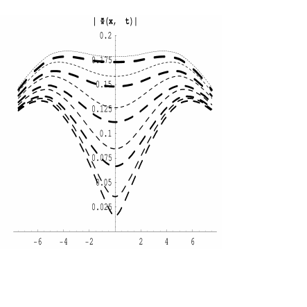
FIG. 5.: The evolution of the field magnitude corresponding to a pair of qballs calculated using the ansatz (28) with $B=4/9$, $\omega_{int}^{2}=0.9$. As time increases the line becomes thicker and the dashes larger. The time range for a complete period of spatial oscillations is $0<t<3$ which implies $\omega_{sp}\simeq 2.1\simeq 2\omega_{int}$ to within 10%.

FIG. 6.: Spatial oscillations of the maximum of the field magnitude due to qball interactions.

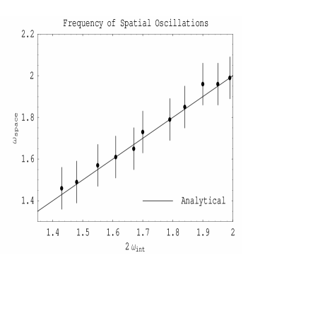
FIG. 7.: The frequency of spatial oscillations of qball position vs the internal frequency of field rotation.

In order to study the scattering of qballs we need to consider boosted qball configurations i.e. qballs moving with a velocity $v$. Starting from a qball field configuration $\Phi_{v=0}(x,t)=\sigma(x)e^{i\omega t}$ which does not move in space we can construct a configuration $\Phi_{v=v_{0}}(x,t)$ that describes a qball moving with velocity $v_{0}$ by performing a Lorenz transform to the spacetime variables. Let $\gamma={1\over{\sqrt{1-v_{0}^{2}}}}$ (we use units where the velocity of light c is unity) be the Lorenz factor and let

$$x^{\prime} = \gamma(x-v_{0}t)$$ (29)

$$t^{\prime} = \gamma(t-v_{0}x)$$ (30)

be the boosted spacetime variables. The field configuration $\Phi(x^{\prime},t^{\prime})$ expressed in terms of $x,\;t$ describes a qball moving with velocity $v_{0}$ i.e. $\Phi_{v=v_{0}}(x,t)=\Phi(x^{\prime},t^{\prime})$. The initial ansatz for a two qball system prepared for a collision process may be written as

$$\Phi(x,t)=\Phi_{v=-v_{0}}(x-x_{0},t)_{\omega_{1}}+\Phi_{v=v_{0}}(x+x_{0},t)_{\omega_{2}}.$$ (31)

An evolved system of this type with $v_{0}=0.2$ is shown in Fig. 8 where we have used $\omega_{1}=\omega_{2}=\sqrt{0.51}$ and $B=4/9$. As it can be seen in Fig. 8 the qball collision results in the formation of a long lived central qball which subsequently decays to qballs similar to the original ones.

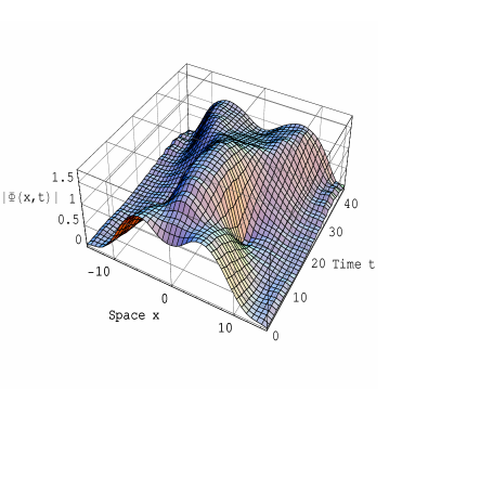
FIG. 8.: Collision of qballs with identical charges and $v_{01}=-v_{02}=0.2$.

A more interesting evolution occurs in two space dimensional systems which will be described in the next section. There it will be seen that the effect of right angle soliton scattering which has been observed in topological solitons persists also in the case of the nontopological qballs in a generalized form.

IV Dynamics in Two Space Dimensions

The model (1) is extended to 2+1 dimensions by letting the index $\mu$ take the values $\mu=0,1,2$. The details of the formalism are similar to those given in Sec. II. That is, the rescaled form of the Lagrangian is given by Eq. (5) while the field equation reads

$${\ddot{\Phi}}-\Delta\Phi+\Phi-|\Phi|\Phi+B|\Phi|^{2}\Phi=0,$$ (32)

where $\Delta=\partial^{2}_{x}+\partial^{2}_{y}$. We look for axially symmetric solutions of Eq. (32) and make the qball ansatz

$$\Phi(\rho,t)=\sigma(\rho)e^{\pm i\omega t},$$ (33)

where $\rho=\sqrt{x^{2}+y^{2}}$. The profile $\sigma(\rho)$ satisfies

$$\sigma^{\prime\prime}+{\sigma^{\prime}\over\rho}+(\omega^{2}-1)\sigma+\sigma^{2}-B\sigma^{3}=0.$$ (34)

FIG. 9.: The numerically calculated profile of the qball solutions for $B=4/9$ and various frequency values. In the vertical axis we plot the charge density $q=\omega\,\sigma^{2}$. Qballs exist for $0.5<\omega^{2}<1$ or $0.71\buildrel<\over{\sim}\omega<1$.

The boundary conditions which have to be met are given in Eqs. (11) and (12). Eq. (34) is expected to have localized solutions by arguments which are presented in [2] and are similar to those used for the 1D model of Sec. II.

The search for the solutions is here not straightforward as for the 1D model (Figs. 1,2). In the present two dimensional case, solutions are found by a numerical shooting method. Fig. 9 shows the profile of the calculated qballs for $B=4/9$ and for various values of the frequency $\omega$. We represent the qball profile through the charge density $q=\omega\,\sigma^{2}$ (cf. Eq. (10)).

The virial theorem mentioned in Sec. II has, for our two dimensional theory, the form

$$I_{3}=I_{1},$$ (35)

where the symbols are defined as the two dimensional analogues of (18) and (20). The virial relation is used to check the precision of our numerical calculations. Indeed, the solutions that we find by the shooting method satisfy the above virial relation to very good precision, better than 1%.

Finally, we note that our shooting method is unable to find the qball profile for the whole frequency range (15). Numerical errors render the method inapplicable near the lower $\omega$-bound. For instance, for $B=2/9$ we are able to find the solutions with $0.035<\omega^{2}<1$ and for $B=4/9$ we find those in the frequency range $0.52<\omega^{2}<1$. The difficulties with the numerics should be anticipated. Their origin can be traced to the theoretical arguments of [2] with respect to the existence of qballs in dimensions higher than one. It is actually the friction term in Eq. (34) which is responsible for the numerical difficulties.

We further note that a steadily moving qball can be found by applying a Lorenz boost to a static one as discussed in the previous section. The calculated qballs will be used in the following in numerical simulations on a two-dimensional lattice. We shall first study their stability. Then we shall study interactions between two qballs, in particular we shall perform simulations of scattering.

The numerical mesh we use is typically $300\times 300$ and the lattice spacing is 0.3. Such a numerical mesh is appropriate to accommodate the structures given in Fig. 9 and provide good resolution. The time evolution is performed by a fourth order Runge-Kutta method.

First, we put a single qball at the center of our numerical mesh and simulate its time evolution in order to test its stability. We use $2/9<B<1$ and test all the values of $\omega$ for which we are able to find the qball profile by our shooting method. We find that qballs are stable everywhere in the $B-\omega$ plane and they travel undistorted with the given constant velocity.

In the next set of simulations we discuss the problem of interaction between qballs. Specifically, we focus on simulations of scattering between two qballs. Such simulations have been performed and have proved to be fruitful for topological solitons. We shall perform all our subsequent numerical simulations using the values $B=4/9$, $\omega=\pm 0.75$.

We consider a 2D generalization of the ansatz (30) which represents two qballs set in a head-on collision course. We use $\omega_{1}=\omega_{2}=0.75$ and a small velocity, namely $v_{0}=0.2$. Qballs are represented through their charge density:

$$q={1\over 2i}(\Phi^{*}\,\partial_{t}\Phi-\Phi\,\partial_{t}\Phi^{*}).$$ (36)

In Fig. 10 contour plots are given for the charge density at three characteristic snapshots of this numerical simulation. The first entry of the figure gives the initial ansatz. The two qballs are initially at a distance of 20 units apart so that there is no overlap and interaction between them. Subsequently they collide at the origin (middle entry) and scatter at right angles (lower entry).

The scattering scenario produced by the computer simulation is quite interesting. Indeed, this dynamical behavior has been found to be a robust feature in a variety of models in two space dimensions which have topological soliton solutions [7, 8]. However, in our case there is no topological invariant associated to the qballs, so we need to discuss it further.

The crucial observation is that the underlying dynamics which induces this type of scattering can be attributed solely to the Hamiltonian structure of the model. It is related to the conservation laws of our model and in particular to the linear momentum conservation [9]. We have followed the linear momentum density plot along the lines described in [9] and we have found a behavior similar to that of topological solitons at the collision time. As a conclusion, despite that in our case there is no topological invariant associated to the qballs, the dynamics related to the right angle scattering behavior is the same as that for their topological counterparts. We should therefore expect such a dynamical behavior to occur generically. We shall study in this section the validity of the above remarks.

FIG. 10.: Head-on collision of two qballs with the same charge. Contour plots of the charge density are given. Contour levels: 0.4, 0.7, 1, 1.3, 1.6, 1.9, 2.2. Three snapshots are shown: initial ansatz (upper entry, time $t=0$), at collision time (middle entry, $t=41.9$) and well after collision (lower entry, $t=55.9$). Parameter values: $B=4/9$, $\omega=0.75$, initial velocity of each qball $v_{0}=0.2$.

FIG. 11.: Head-on collision of two qballs with the same charge. Contour plots of the charge density are given. Contour levels: 0.4, 0.8, 1.2, 1.6, 2.4, 3.2. Snapshots at: $t=0$ (upper entry), $t=19.6$ (middle entry) and $t=69.8$ (lower entry). Initial velocity of each qball $v_{0}=0.4$. Rest of parameters as in Fig. 10.

Following the simulation for later times, the two qballs are seen to eventually stop along the $y$-axis. They then attract, collide again and subsequently scatter and re-emerge on the $x$-axis. This scenario goes on and gives an oscillating system with successive right angle scattering. We shall not pursue further here this oscillating behavior.

The next simulation we present has been prepared in a way similar to the previous one, but now the initial

FIG. 12.: Head-on collision of two qballs with the same charge. Contour plots of the charge density are given. Contour levels: 0.4, 0.8, 1.6, 2.4, 5, 8. Snapshots at: $t=0$ (upper entry), $t=12.6$ (middle entry) and $t=29.3$ (lower entry). Initial velocity of each qball $v_{0}=0.8$. Rest of parameters as in Fig. 10

velocity of the qballs is set to a higher value $v_{0}=0.4$. The results are shown in Fig. 11. At the initial stages, the simulation does not differ from our first simulation. At collision time (middle entry) a central qball is formed. However, the subsequent evolution is considerably different. In the lower entry of the figure we have two qballs which have evolved from a right angle scattering process. They are located on the $y$-axis and are almost static. In addition to that, two other qballs are continuing their route along the $x$-axis and they are drifting away from each other. Their drift velocity is approximately 0.24.

It would be interesting to have some insight in the above described process. The basic remark is that the symmetry that has lead to the right angle scattering in the first (slow qballs) case, leads here again to the same result. On the other hand, the high kinetic energy of the initial qballs allows for more complicated scenarios like the formation of new qballs. That is, some amount of energy that does not follow the right angle scenario, reorganizes to form qballs on the $x$-axis. In the case of topological soliton interactions, arguments related to topology would usually preclude such scenarios. These arguments do not apply in the case of qballs thus we are led to a novel result. An interesting observation is that the four solitons which are created after the collision seem to be qballs with a frequency different than that of the initial ones. This can be seen by comparing the last entry of Fig. 11 with the profiles of qballs of various frequencies, obtained by our numerical shooting method.

We have repeated the above scattering numerical experiment with qballs of higher initial velocity $v_{0}=0.8$. The results of the simulation are given in Fig. 12. A new type of collision different than in the two previous cases arises. The qballs actually collide to form a central qball at the origin (middle entry of the figure). However, after the collision (lower entry of the figure) two qballs re-emerge traveling along the $x$-axis and drifting away from each other. Their drift velocity after collision is approximately 0.75. No right angle scattering is present in this case so the qballs appear to be almost non-interacting. This result is dramatically different from what we see in the case of the slow qballs of Fig. 10 where pure right angle scattering occurs. It resembles however similar results discussed in the literature for scattering of topological solitons moving with very high relativistic velocities[10].

Notice also that Ward’s chiral model, which is integrable in 2+1 dimensions, presents in some respects similar dynamical behavior. Specifically, it has solutions which correspond to the right angle scattering [8] and others which represent noninteracting solitons [11] although the velocity of the solitons does not seem to play any role there. On the other hand, the type of scattering shown in Fig. 11 seems to be specific to nontopological solitons and, to our knowledge, it has not been observed in other two-dimensional models.

The right angle scattering of solitons has also been observed in a three-dimensional Yang-Mills-Higgs theory [12]. The problem has been approached within the moduli space, that is, the space of the multi-monopole solutions in the Bogomonly limit. It has been stressed that the scattering behavior of the monopoles can be understood when they are considered almost static during the interaction. This requires that the velocity of the interacting monopoles is small. Such is certainly the case with the first of our simulations here shown in Fig 10.

FIG. 13.: Head-on collision of two qballs with opposite charge. Contour plots of the charge density are given. Solid lines represent positive values and dashed-dotted lines negative values. Contour levels: $\pm 0.2,\pm 0.4,\pm 0.8,\pm 1.2,\pm 1.6$. Snapshots at: $t=0$ (upper entry), $t=28$ (middle entry) and $t=61.4$ (lower entry). Initial velocity of each qball $v_{0}=0.4$. Rest of parameters as in Fig. 10

Additional insight in the dynamics can be gained by looking at collisions between qballs of opposite charge. Such are two qballs with the same profile and opposite field precession frequency (cf. Eq. (33)). Notice that the arguments of [9] can not be applied in this case, at least not in a straightforward manner. In particular, these arguments indicate that we may not expect that the two initial qballs can re-emerge after collision, traveling at a direction perpendicular to the initial one. Rather, we would have to think of a combination of parts of the initial qballs which would form the final solution after collision. Such a combination, involving parts of qballs with opposite charge, does not seem to form any solution of the present theory, therefore we don’t expect a right angle scattering behavior in the current case. We have to resort to numerical simulations in order to determine the actual behavior of the system.

We now use an initial ansatz appropriately chosen to account for opposite-charge qball collision. This ansatz is shown in the upper entry of Fig. 13 through contour plots of the charge density. The positive-charge qball is located on the left of the figure and the negative-charge one on the right. We apply to each of the initial qballs a Lorenz boost with a moderate velocity $v_{0}=0.4$. The middle entry of the figure shows that, quite interestingly, at the time of collision a mixed state is formed between the two qballs. After that, the two qballs separate again, they appear to pass through each other and drift apart. The final qballs are not identical to the initial ones. The charge Q of each of them is approximately half of that of the initial state and it corresponds to a frequency $\omega\sim\pm 0.6$. They have also decelerated and their mean velocity is approximately equal to 0.25.

In Sec. II, we have found an interaction between the pair of oppositely charged qballs which introduces an oscillation frequency to the system equal to twice the qball internal frequency. This interaction is present here and it manifests itself in oscillations of the magnitude of the field values and also in oscillations of the position of the qball centers. The oscillations appear when the qballs are coming close to collide. They also persist after the collision even when the qballs are well separated (i.e. at the instant of the last entry of Fig. 13) and they don’t show any tendency to fade out.

Computer plots of the distribution of the energy density of the system shows that some small amount of energy is dissipated at right angles after collision. The underlying mechanism for this phenomenon is presumably similar to that leading to right angle scattering in the first of our simulations in this series. Similar behavior has been observed for two colliding topological solitons with opposite topological charge [10]. In this case, the solitons annihilate and the energy is dissipated at right angles.

The scattering behavior described by the simulations of this section can be viewed as a generalization of the corresponding behavior of topological solitons. We observe the two extreme cases which have also been observed in the topological case (pure right angle scattering at low velocities and pure forward scattering at very high velocities) but we also observe an intermediate case of a qball split to a forward and a right angle scattering component at intermediate velocities. The forward scattering component gets amplified at high collision velocities. This amplification occurs at the expense of the right angle scattering component.

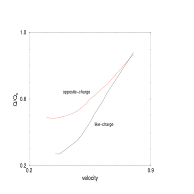
FIG. 14.: The fractional charge in forward scattering of qballs as a function of the rest frame qball velocity. The forward component is clearly amplified at large velocities. Points in the figure are plotted every 0.25 velocity units. Then the points are connected by straight lines.

The rich behavior of qballs in the scattering simulations calls for an overview of the different phases.

• Low velocity scattering of qballs with the same charge leads to initial right angle scattering and a bound system that performs breather type oscillations.

• Intermediate velocity scattering ($0.3<v<0.7$) leads to a combination of forward and right angle scattering and the forward scattered qballs drift away from each other and escape to infinity.

• High velocity scattering ($v>0.7$) leads to pure forward scattering. The forward scattered qballs drift away from each other and escape to infinity.

To clarify the transition from pure right angle scattering to pure forward scattering in the case of identically charged non-topological solitons we plot (Fig. 14) the charge of each of the forward scattered qballs as a fraction of the initial qball charge, versus the initial velocity . Since the total charge is conserved the rest of the charge is scattered at right angles. A small amount is dissipated throughout our lattice.

The charge of the outgoing qballs is computed as follows: We let the qballs travel 30 space units on the $x$-axis, after the collision and we integrate the charge density within a disc of radius 15 space units around each qball center. This result is considered to be the charge of the final qballs.

In the case of scattering of oppositely charged qballs we have also observed an increase of the forward scattered component charge for high velocities (upper curve of Fig. 14). This increase however does not occur due to reduced right angle scattering (this does not happen in this case) but due to reduced annihilation between the opposite qball charges which is a result of the reduced time of overlap between the fast moving qball profiles.

V Conclusion - Outlook

We have studied the stability and the dynamics of qballs in the context of a simple toy model. We have found that the qball instability sector is a very small sector in parameter space. The validity of a virial theorem in the stability sector has also been verified and we have shown that systems of qball pairs tend to perform breather-type oscillations for long time periods compared to the period of the internal field rotation. Finally we have studied numerically the scattering of qball pairs and found that qballs in two space dimensions with the same charge tend to scatter at right angles and subsequently perform oscillations with repeated collisions through right angle scattering. At relativistic collision velocities a significant forward scattering component has also been found which gets amplified as the collision velocity increases. This effect is consistent with numerical experiments involving topological solitons where the charge is discretized due to topology. In that case complete forward scattering is found for $v>v_{crit}\simeq 0.9$[10]. In the nontopological case the smooth interpolation between the above two regimes is allowed because the charge is not discretized.

These results are interesting not only in the context of the general study of the solitonic dynamical properties but also in the context of realistic physical systems. For example in a cosmological setup where dark matter comes from susy qballs, breather-type large qball systems could lead to detectable signatures in the gravitational wave spectrum either by direct emission or by exciting vibration modes of the neutron stars where they can be trapped[13]. The detectable characteristics of such breather type cosmological systems are currently under investigation. Another interesting implication is related to the statistical mechanics of qball systems[4]. Our results imply that the number of qballs is not conserved in such systems and in fact it may increase rapidly during multiple high velocity collision processes. This is in contrast with the assumptions made in recent work [5] which assumes that merging is the only possible outcome of qball collisions.

A natural extension of our work is the numerical study of the formation of qballs during a (cosmological) phase transition. Such studies based on numerical simulation s[14, 15] of a system though a temperature quench have been performed extensively in the context of topological solitons [15, 16] but not in the context of nontopological configurations like the ones considered in the present study. Mechanisms of thermal creation and annihilation of nontopological solitons in the aftermath of a phase transition have been previously studied. For small Q balls it is assummed their fusion into larger ones to be dominant for both high and low thermal reaction rates [17] Clearly our results modify the above picture in an interesting way. The numerical simulations performed here can be extended in a straightforward way to apply to the case of qball formation during a quench. The realization of this extension is currently in progress.

VI Acknowledgements

We thank N. Papanicolaou for useful conversations

REFERENCES

- [1] T.D. Lee and Y. Pang, Phys. Rept. 221 (1992) 251
- [2] S. Coleman, Nucl. Phys. B262 (1985) 263
- [3] A. Kusenko, Phys. Lett. B404 (1997) 285,
- [4] A. Kusenko, Nucl. Phys. Proc. Suppl. 62A/C (1998) 248, G. Dvali, A. Kusenko and M. Shaposhnikov, Phys.Lett. B417 (1998) 99; K. Enqvist and J. McDonald, Phys. Lett. B425 (1998) 309; ibid Nucl. Phys. B538, (1999)3221, A. Kusenko, M.Shaposhnikov, P.G. Tinyakov and I.G.Tkachev, Phys. Lett. B423, A. Kusenko, V. Kuzmin, M. Shaposhnikov and P.G. Tinyakov, Phys. Rev. Lett. 80 (1998) 3185, M. Axenides, E.G. Floratos and A. Kehagias, Phys. Lett B444
- [5] A. Kusenko and M. Shaposhnikov, Phys. Lett. B418, (1998) 104.
- [6] G.H. Derrick, J. Math Phys. 5, 1252 (1964)
- [7] P.J. Ruback, Nucl. Phys. B 296 (1988) 669
-
[8]
R.S. Ward, Phys. Lett A 208 (1995) 203;
T. Ioannidou and W.J. Zakrzewski, J. of Math. Phys. 39 (1998) 2693 - [9] S. Komineas, ”Scattering of solitons in two dimensions” cond-mat/9904093.
- [10] E.P.S. Shellard, Nucl. Phys. B 283 (1987) 624
- [11] R.S. Ward, J. Math. Phys. 29 (1988) 386
-
[12]
N.S. Manton, Phys. Lett B 110 (1982) 54;
N.J. Hitchin, N.S. Manton and M.K. Murray, Nonlinearity 8 (1995) 661 - [13] J. Madsen, Phys. Lett. B435 (1998) 125, hep-ph/9806433
- [14] J.Ye and R.H.Brandenberger, Mod. Phys. Lett. A5 (1990) 157; Nucl. Phys. B346 (1990) 149
- [15] W.H. Zurek, Phys. Rept. 276 (1996) 177, cond-mat/9607135
- [16] P. Laguna and W.H. Zurek, Phys. Rev. Lett. 78 (1997) 2519, gr-qc/9607041
- [17] J.A. Frieman, G.B. Gelmini, M. Gleiser and E.W. Kolb, Phys. Rev. Letts 60, 2101 (1988); K. Griest and E.W. Kolb, Phys. Rev. D40, 3231 (1989); J.A. Frieman, A.V. Olinto, M. Gleiser and C. Alcock, Phys. Rev. D40, 3241 (1989).