Abstract

We discuss the Overhauser effect (particle-hole pairing) versus the BCS effect (particle-particle or hole-hole pairing) in QCD at large quark density. In weak coupling and to leading logarithm accuracy, the pairing energies can be estimated exactly. For a small number of colors, the BCS effect overtakes the Overhauser effect, while for a large number of colors the opposite takes place, in agreement with a recent renormalization group argument. In strong coupling with large pairing energies, the Overhauser effect may be dominant for any number of colors, suggesting that QCD may crystallize into an insulator at a few times nuclear matter density, a situation reminiscent of dense Skyrmions. The Overhauser effect is dominant in QCD in 1+1 dimensions, although susceptible to quantum effects. It is sensitive to temperature in all dimensions.

KIAS-P99047
FZJ-IKP(TH)-1999-27

1. Introduction

Quantum chromodynamics (QCD) at high density, relevant to the physics of the early universe, compact stars and relativistic heavy ion collisions, is presently attracting a renewed attention from both nuclear and particle theorists. Following an early suggestion by Bailin and Love [1], it was recently stressed that at large quark density, diquarks could condense into a color superconductor [2], with potentially interesting and novel phenomena such as color-flavor locking, chiral symmetry breaking, parity violation, color-flavor anomalies, and superqualitons.

At large density, quarks at the edge of the Fermi surface interact weakly thanks to asymptotic freedom. However, the high degeneracy of the Fermi surface causes perturbation theory to fail. As a result, particles can pair and condense at the edge of the Fermi surface leading to energy gaps. Particle-particle and hole-hole pairing (BCS effect) have been extensively studied recently [1, 2]. Particle-hole pairing at the opposite edges of the Fermi surface (Overhauser effect) [3] has received little attention with the exception of an early variational study by Deryagin, Grigoriev and Rubakov for a large number of colors [4], and a recent renormalization group argument in [5]. The scattering amplitude between a pair of particles at the opposite edges of the Fermi surface peaks in the forward direction, a situation reminiscent of the forward enhancement in Compton and Bhabha scattering.

In retrospect, it is surprising that the Overhauser effect in QCD has attracted so little attention. In fact, the Schwinger model [6] shows that when a uniform external charge density is applied, the electrons respond by screening the external charge and inducing a charge density wave, a situation analogous to a Wigner crystal  [7, 8, 9]. Similar considerations apply to QCD in 1+1 dimensions [8]. In 3+1 dimensions, dense Skyrmion calculations with realistic chiral parameters yield a 3-dimensional Wigner-type crystal with half-Skyrmion symmetry at few times nuclear matter density [10, 11]. At these densities, Fermi motion is expected to be overtaken by the classical interaction [12]. A close inspection of these results shows the occurrence of scalar-isoscalar, pseudoscalar-isovector and vector-isoscalar charge density waves in an ensemble of dense Skyrmions.

In this paper we will show that in dense QCD, the equations that drive the particle-hole instability at the opposite edge of a Fermi surface resemble those that drive the particle-particle or hole-hole instability in the scalar-isoscalar channel, modulo phase-space factors. In section 2 we motivate and derive a Wilsonian action around the Fermi surface. In section 3 we obtain expressions for the energy densities and pertinent gaps in the $0^{+}$ channel with screening, thereby generalizing the original results in [4]. In section 4, we analyze the decoupled equations for large chemical potential without screening. The effects of screening for arbitrary $N_{c}$ as well as temperature are discussed in section 5, in overall agreement with a recent renormalization group argument [5]. In section 6, we discuss the Overhauser effect in QCD in lower dimensions. Our conclusions and suggestions are given in section 7.

2. Effective Action at the Fermi Surface

To compare the Overhauser effect to the BCS effect, we will construct a Wilsonian effective action by integrating out the quark modes around the Fermi surface, in the presence of smooth bilocal fields. An alternative would be the quantum action [13]. At large chemical potential, most of the Fermi surface is Pauli-blocked, so the quasiparticle content of the theory is well described by such an action. Incidentally, our analysis should provide a useful alternative to a brute-force lattice QCD analysis. Indeed, an effective formulation of lattice QCD along the lines of the heavy-quark formalism is possible and will be discussed elsewhere [14].

The starting point in our analysis is the appropriate QCD action in Euclidean space with massless quarks

$$S=\int d^{4}x\,\left[\frac{1}{4}(F_{\mu\nu}^{a})^{2}+\bar{\psi}(\gamma_{\mu}\partial_{\mu}-\gamma_{4}\mu)\psi-iJ^{a}_{\mu}A^{a}_{\mu}\right]\;,$$ (1)

and the colored current

$$J_{\mu}^{a}=g\bar{\psi}\gamma_{\mu}\frac{\lambda^{a}}{2}\psi\;.$$ (2)

In Euclidean space, our conventions are such that the $\gamma$-matrices are hermitean with $\{\gamma_{\mu},\gamma_{\nu}\}=2\delta_{\mu\nu}$. For sufficiently large $\mu$, we will assume $g^{2}N_{c}\ll 1$. We have omitted gauge-fixing terms and ghost-fields. In what follows, we will analyze (1) in the one-loop approximation with the gluon field in the Feynman gauge. The approximation, as we shall show below, is equivalent to the resummation of the ladder graphs in the particle-particle or particle-hole graphs. The effects of screening will be dealt with by minimally modifying the gluon propagator, ignoring for simplicity vertex corrections as in [2]. The issue of gauge fixing dependence will be briefly discussed at the end.

In the one-loop approximation with screened gluons, the induced action is

$$S_{\psi}=\frac{g^{2}}{2}\int d^{4}x\,d^{4}y\,J^{a}_{\mu}(x){\cal D}_{\mu\nu}(x-y)J^{a}_{\nu}(y)+\int d^{4}x\,\bar{\psi}\,\tilde{\partial}_{\mu}\gamma_{\mu}\psi\;,$$ (3)

where $\tilde{\partial}_{\mu}=(\partial_{1},\partial_{2},\partial_{3},\partial_{4}-\mu)$. The screened gluon propagator $\{{\cal D}_{\mu\nu}\}=({\cal D}_{E},{\cal D}_{M})$ is

$${\cal D}_{E,M}(x-y)=\int\frac{d^{4}q}{(2\pi)^{4}}\,\frac{1}{q^{2}+m_{E,M}^{2}}e^{-iq\cdot(x-y)}\;.$$ (4)

Perturbative arguments give $m_{E}^{2}/(g\mu)^{2}=m_{D}^{2}/(g\mu)^{2}\approx N_{f}/2\pi^{2}$ and $m_{M}^{2}/m_{D}^{2}\approx\pi{|q_{4}|/|4{\bf q}|}$, where $m_{D}$ is the Debye mass, $m_{M}$ is the magnetic screening generated by Landau damping and $N_{f}$ the number of flavors [15] . Nonperturbative arguments suggest $m_{E}^{2},m_{M}^{2}\rightarrow m_{*}^{4}/q^{2}$ [16] where for simplicity, the difference between electric and magnetic channels is ignored. We expect $\Lambda_{QCD}\ll m_{*}<m_{E}$ in the case $N_{c}=3$, as lattice simulations for the gluon propagator at finite $\mu$ are not yet available. We note that the perturbative screening vanishes at large $N_{c}$.

To proceed further with (3) we need to Fierz rearrange the $JJ$ term in (3). This is equivalent to summing ladder graphs with relevant quantum numbers. Specifically,

$$J^{a}_{\mu}(x){\cal D}_{\mu\nu}(x-y)J^{a}_{\nu}(y) = g^{2}\sum_{\cal O}\,\,{\cal C}_{\cal O}\left[\bar{\psi}(x){\bf M}_{\cal O}\psi(y)\right]\,{\cal D}(x-y)\,\left[\bar{\psi}(y){\bf M}_{\cal O}\psi(x)\right]$$ (5)

$$+ g^{2}\sum_{{\cal O^{\prime}}}\,\,{\cal C}_{{\cal O}^{\prime}}\left[\bar{\psi}(x){\bf M}_{{\cal O}^{\prime}}\psi^{c}(y)\right]\,{\cal D}(x-y)\,\left[\bar{\psi}^{c}(y){\bf M}_{{\cal O}^{\prime}}\psi(x)\right]$$

with ${\cal C}_{O}=-1/9$ and ${\cal C}_{C}=+1/36$ for the operators

$$\left[\bar{\psi}(x)\,{\bf M}_{O}\,\psi(y)\right] = \bar{\psi}_{\alpha,a,i}(x)\,\delta_{\alpha\beta}\,\delta_{ab}\delta_{ij}\,\psi_{\beta,b,j}(y)\;,$$

$$\left[\bar{\psi}(x)\,{\bf M}_{C}\,{\psi}^{c}(y)\right] = \bar{\psi}_{\alpha,a,i}(x)\,(\gamma_{5})_{\alpha\beta}\,\varepsilon^{I}_{ab}\varepsilon^{I}_{ij}\,C\bar{\psi}^{T}_{\beta,b,j}(y)\;,$$ (6)

respectively, with $N_{f}=N_{c}=3$. These quantities involve matrices active in color $(a,b,\cdots)$, flavor $(i,j,\cdots)$ and Dirac space $(\alpha,\beta,\cdots)$. ${\bf M}_{O}$ is the vertex generator for particle-hole pairing in the $0^{+}$ channel (i.e., Overhauser), while ${\bf M}_{C}$ is the vertex generator for particle-particle and hole-hole pairing in the color-flavor locked (CFL) channel (i.e., BCS). Only these two operators will be retained below, unless specified otherwise. The gluon-propagator in matter is

$${\cal D}(x-y)=\textstyle\frac{1}{2}{\cal D}_{E}(x-y)+\frac{1}{2}{\cal D}_{M}(x-y)\;.$$ (7)

The weightings follow from minimal substitution in matter with 2 electric and 2 magnetic modes. We note that the present Fierzing is particular, since it selects solely the ${\bf 1}_{c}$ in the $\overline{q}q$ channel and the $\overline{\bf 3}_{c}$ in the $qq$ channel [17]. For arbitrary $N_{c}\geq 3$ and $N_{f}\geq 2$, the coefficients $-\textstyle\frac{1}{9}$ and $\textstyle\frac{1}{36}$ become, respectively, $-\frac{1}{2}(1-\frac{1}{N_{c}})\cdot\frac{1}{N_{f}}$ and $\frac{1}{2N_{c}}\cdot\frac{1}{2}\cdot\frac{1}{\min(N_{c},N_{f})}$, where the single factors refer, in turn, to the results of the color Fierzing, the flavor Fierzing and, of course only for the second expression, the Fierzing related to color-flavor locking . To compare to the more conventional decompositions through ${\bf 3}_{c}\times\overline{\bf 3}_{c}={\bf 1}_{c}+{\bf 8}_{c}$ for $\overline{q}q$ and ${\bf 3}_{c}\times{\bf 3}_{c}=\overline{\bf 3}_{c}+{\bf 6}_{c}$ for $qq$, with respective weights $-\frac{1}{2}(1-\frac{1}{N_{c}^{2}})\cdot\frac{1}{N_{f}}$ and $\frac{N_{c}+1}{4N_{c}}\cdot\frac{1}{2}\cdot\frac{1}{\min(N_{c},N_{f})}$, we introduce also the vertex generator [2]

$$\left[\bar{\psi}(x)\,{\bf M}_{B}\,{\psi}^{c}(y)\right]=\bar{\psi}_{\alpha,a,i}(x)\,(\gamma_{5})_{\alpha\beta}\,(\lambda_{2})_{ab}(\tau_{2})_{ij}C\bar{\psi}^{T}_{\beta,b,j}(y)\;.$$ (8)

We note that (8) does not lock color and flavor as it stands; a color-flavor locking as described in footnote #2 still has to be performed, such that finally the corresponding coefficient becomes ${\cal C}_{B}=(N_{c}+1)/\{8N_{c}\min(N_{f},N_{c})\}$ . This brings about the important issue of whether Fierzing is a unique operation on 4-fermi interactions. The answer is no [22, 23]. This nonuniqueness would of course not be important if an all-order calculation were to be performed for any Fierzing set, but is of course relevant for truncated calculations as is the case in general. Each Fierzing corresponds to summing a specific class of ladder diagrams in the energy density, see e.g. [22, 23].

Introducing a hermitian bilocal field $\Sigma(x,y)$ and a non-hermitian bilocal field $\Gamma(x,y)$, we may linearize the Fierzed form of the $JJ$ term by using the Hubbard-Stratonovich transformation, e.g.

$$\exp\left(\textstyle\frac{g^{2}}{18}\displaystyle\int d^{4}x\,d^{4}y\,\left[\bar{\psi}(x)\psi(y)\right]{\cal D}(x-y)\left[\bar{\psi}(y)\psi(x)\right]\right)$$ (9)

$$= \int d\Sigma(x,y)\,\exp\left(-S_{\Sigma}-\int d^{4}x\,d^{4}y\,\bar{\psi}(x)\,\Sigma(x,y)\,\psi(y)\right)$$

with

$${S}_{\Sigma}=\frac{9}{2g^{2}}\int d^{4}x\,d^{4}y\,\frac{\left|\Sigma(x,y)\right|^{2}}{{\cal D}(x-y)}$$ (10)

and similarly for $\Gamma$. As a result, the action in the quark fields is linear and the functional integration can be performed. The result is the following effective action for the bilocal fields

$${S}={S}_{\Sigma}+{S}_{\Gamma}-{\textstyle\frac{1}{2}}\mbox{Tr}{\ }\mbox{ln}{\bf F}\;,$$ (11)

where

$${\bf F}=\left(\begin{array}[]{cc}\left\{\gamma\cdot{\partial}-\mu\gamma_{4}\right\}\delta(x-y)+{\bf M}_{O}\Sigma(x,y)&i\Gamma^{\dagger}(x,y)C^{T}{\bf M}_{C}\\ iC^{T}\Gamma(x,y){\bf M}_{C}&\left\{\gamma\cdot{\partial}+\mu\gamma_{4}\right\}\delta(x-y)+{\bf M}_{O}\Sigma(x,y)\end{array}\right).$$ (12)

The factor of $1/2$ in (11) is due to the occurrence of $\psi$ and $\psi^{c}$ through the Fierzing into ${\bf 1}_{c}$ and ${\bf 3}_{c}$ [17]. This renders naturally the Gorkov formalism applicable to the present problem even at $\mu=0$. Note that ${\bf M}_{O}={\bf 1}_{C}\times{\bf 1}_{F}\times{\bf 1}_{D}$ and ${\bf M}_{C}=\varepsilon_{C}^{I}\times\varepsilon_{F}^{I}\times\gamma_{5}$, with the subscripts $C,F,D$ short for color, flavor and Dirac. We should stress that the effective action (11) is general. The third term is the Hartree contribution of the quarks to the ground state energy at large chemical potential, while the first two terms remove the double counting in the potential (i.e., Fock terms).

To analyze the Overhauser and BCS effects in parallel, we make simplifying ansätze for the bilocal auxiliary fields. Since the unscreened gluon interaction in both cases peak in the forward direction, we may choose

$$\Sigma(x,y) \!=\! 2\cos\left[P_{\mu}\left(\frac{x_{\mu}+y_{\mu}}{2}\right)\right]\sigma(x-y)=2\cos\left[P_{\mu}\left(\frac{x_{\mu}+y_{\mu}}{2}\right)\right]\int\frac{d^{4}q}{(2\pi)^{4}}\,e^{-iq\cdot(x-y)}F(q)\;,$$

$$\Gamma(x,y) \!=\! 2\cos\left[P_{\mu}\left(\frac{x_{\mu}-y_{\mu}}{2}\right)\right]g(x-y)=2\cos\left[P_{\mu}\left(\frac{x_{\mu}-y_{\mu}}{2}\right)\right]\int\frac{d^{4}q}{(2\pi)^{4}}\,e^{-iq\cdot(x-y)}G(q)\;,$$

where ${P_{\mu}}=({\bf P}_{F},0)$ and $|{\bf P}_{F}|=2\mu$. ${\bf P}_{F}$ points in the original direction of one of the quark. $F(q)$ and $G(q)$ are even functions, $F(q)$ is real, since $\Sigma(x,y)=\Sigma(y,x)^{\ast}$, and $G(q)$ is complex, since $\Gamma^{\dagger}(x,y)=\Gamma(y,x)^{\ast}$. The relative momentum $q$ satisfies $|q|\leq|P/2|=\mu$. The bilocal field $\Gamma$ characterizes a BCS pair of zero total momentum. $\Sigma$ characterizes a wave of total momentum $2\mu$. This is the optimal choice for the momentum of the standing wave for which the holes contribute coherently to the wave formation. As a result the gap opens up at the Fermi surface, with $\mu$ as the divide between particles and holes. In both cases, the pairing involves a particle and/or hole at the opposite sides of the Fermi surface. Indeed, in terms of (LABEL:S14) the linear terms in the bilocal fields are

$$\int d^{4}x\,d^{4}y\,\bar{\psi}(x)\Sigma(x,y)\psi(y)$$ (14)

$$= V_{4}\int\frac{d^{4}q}{(2\pi)^{4}}\,\left[\bar{\psi}\left(-\frac{P}{2}\mbox{+}q\right)\,F(q)\,\psi\left(\frac{P}{2}\mbox{+}q\right)+\bar{\psi}\left(\frac{P}{2}\mbox{+}q\right)\,F(q)\,\psi\left(-\frac{P}{2}\mbox{+}q\right)\right]$$

(see Ref.[4]) and

$${\textstyle\frac{1}{2}}\int d^{4}x\,d^{4}y\,\left[\bar{\psi}^{c}(x)i\gamma_{5}\Gamma(x,y)\psi(y)+\bar{\psi}(x)\Gamma^{\dagger}(x,y)i\gamma_{5}\psi^{c}(y)\right]$$ (15)

$$\!\!=\!\! \!{\textstyle\frac{1}{2}}V_{4}\!\int\!\frac{d^{4}q}{(2\pi)^{4}}\left[\psi^{T}\left(-\frac{P}{2}\mbox{$-$}q\right)Ci\gamma_{5}G(q)\,\psi\left(\frac{P}{2}\mbox{+}q\right)+\bar{\psi}\left(\frac{P}{2}+q\right)iG^{\ast}(q)\gamma_{5}C\psi^{T}\left(-\frac{P}{2}\mbox{$-$}q\right)\right.$$

$$\;\mbox{+}\left.\psi^{T}\left(\frac{P}{2}\mbox{$-$}q\right)\,Ci\gamma_{5}G(q)\,\psi\left(-\frac{P}{2}\mbox{+}q\right)+\bar{\psi}\left(-\frac{P}{2}\mbox{+}q\right)\,iG^{\ast}(q)\gamma_{5}C\psi^{T}\left(\frac{P}{2}\mbox{$-$}q\right)\right],$$

where $V_{4}$ is the 4-volume.

Following [4], we introduce fermion fields $\psi(\pm P/2+q)$ and $\psi^{c}(\pm P/2-q)$  that are independent integration variables in the relevant region of the momentum $|q|\ll|{\bf P}|/2$. Hence, the quark contribution around the Fermi surface can be integrated. The result is [25]

$$\det{\bf F}={\rm exp}\left(V_{4}\,{\rm Tr\,\,ln}\left|{\begin{array}[]{cccc}-i\widetilde{Q}_{+,\mu}{\bf\sigma}_{\mu}&F(q)&iG^{\ast}(q)\,\,{\bf M}_{C}&{\bf 0}\\ F(q)&-i\widetilde{Q}_{-,\mu}{\bf\bar{\sigma}}_{\mu}&{\bf 0}&-iG^{\ast}(q)\,\,{\bf M}_{C}\\ -iG(q)\,\,{\bf M}_{C}&{\bf 0}&-i\widetilde{Q}_{+,\mu}^{*}{\bf\bar{\sigma}}_{\mu}&F(-q)\\ {\bf 0}&iG(q)\,\,{\bf M}_{C}&F(-q)&-i\widetilde{Q}_{-,\mu}^{*}{\bf\sigma}_{\mu}\end{array}}\right|\,\right)\;,$$ (20)

where $Q_{\pm}\equiv\pm\frac{P}{2}+q$ and $\widetilde{Q}_{\pm}\equiv\left({\bf Q}_{\pm}\,\,,\,Q^{4}_{\pm}-i\mu\,\right)$. For each entry in momentum space $q$, the determinant in (20) is over an $(8\cdot N_{c}\cdot N_{f})\times(8\cdot N_{c}\cdot N_{f})$-matrix. The matrices $\sigma_{\mu}=(i\,{\vec{\sigma}}\,,\,{\bf 1})$ and $\bar{\sigma}_{\mu}=(-i\,{\vec{\sigma}}\,,\,{\bf 1})$ are defined in terms of the usual Pauli matrices ${\vec{\sigma}}$. The detailed analysis of the coupled problem (20) with the full Fermion determinant will be discussed elsewhere [25].

3. Gap Equations

A qualitative understanding of the Overhauser effect versus the BCS effect can be achieved by studying the phases separately, and then comparing their energy densities at large quark density. Setting $G=0$ yields, for the Overhauser pairing, an energy density

$$\frac{{S}_{\Sigma}}{9V_{4}}=\frac{1}{g^{2}}\int d^{4}x\,\frac{|\sigma(x)|^{2}}{{\cal D}(x)}-2\int\frac{d^{4}q}{(2\pi)^{4}}\,\ln\left[\frac{\tilde{Q}_{+}^{2}\tilde{Q}_{-}^{2}+2F^{2}\,\tilde{Q}_{+}\tilde{Q}_{-}+F^{4}}{\tilde{Q}_{+}^{2}\tilde{Q}_{-}^{2}}\right]\equiv{\cal S}_{\mbox{\scriptsize pot},\Sigma}+{\cal S}_{\mbox{\scriptsize kin},\Sigma}$$ (21)

which is in agreement with the result derived originally in [4]. Setting $F=0$ yields, for the BCS pairing, an energy density

$$\frac{{S}_{\Gamma}}{36V_{4}}=\frac{1}{g^{2}}\int d^{4}x\,\frac{|g(x)|^{2}}{{\cal D}(x)}-\frac{2}{3}\int\frac{d^{4}q}{(2\pi)^{4}}\,\ln\left[\frac{\tilde{Q}_{+}^{2}\tilde{Q}_{+}^{\ast 2}+2|G|^{2}\,\tilde{Q}_{+}\tilde{Q}_{+}^{\ast}+|G|^{4}}{\tilde{Q}_{+}^{2}\tilde{Q}_{+}^{*2}}\right]\equiv{\cal S}_{\mbox{\scriptsize pot},\Gamma}+{\cal S}_{\mbox{\scriptsize kin},\Gamma}$$ (22)

which is similar to (21). In writing the last equation we have assumed that $|G(q\pm P)|\approx|G(\pm\mu)|\approx 0$. The gap equations for both cases follow by variation. The result is

$$F(p)=2g^{2}\int\frac{d^{4}q}{(2\pi)^{4}}\,{\cal D}(p-q)\left(\frac{2F(q)\left(\tilde{Q}_{+}\tilde{Q}_{-}+F^{2}(q)\right)}{\tilde{Q}_{+}^{2}\tilde{Q}_{-}^{2}+2F^{2}(q)\,\tilde{Q}_{+}\tilde{Q}_{-}+F^{4}(q)}\right)$$ (23)

for the Overhauser gap, and

$$G(p)={\textstyle\frac{2}{3}}g^{2}\int\frac{d^{4}q}{(2\pi)^{4}}\,{\cal D}(p-q)\left(\frac{2G(q)\left(\tilde{Q}_{+}\tilde{Q}_{+}^{\ast}+|G(q)|^{2}\right)}{\tilde{Q}_{+}^{2}\tilde{Q}_{+}^{*2}+2|G(q)|^{2}\,\tilde{Q}_{+}\tilde{Q}_{+}^{\ast}+|G(q)|^{4}}\right)$$ (24)

for the BCS gap. If we were to use the antisymmetric vertex operator (8) then we would have $2g^{2}/3\rightarrow 4g^{2}/3$. For the latter, we have checked that the results (23-24) agree with the Bethe-Salpeter derivation in the ladder approximation to order $\mu^{0}$. In our notations, the leading order effects are of order $\mu$, the next to leading order effects are of order $\mu^{0}$ and the next-to-next to leading order effects are of order $\mu^{-1}$. For the screened gluon propagator we have the alternatives

$${\cal D}(q)=\textstyle\frac{1}{2}\displaystyle\frac{1}{q^{2}+m_{E}^{2}}+\textstyle\frac{1}{2}\displaystyle\frac{1}{q^{2}+m_{M}^{2}}\;,$$

$${\cal D}(q)=\textstyle\frac{1}{2}\displaystyle\frac{1}{q^{2}+im_{*}^{2}}+\textstyle\frac{1}{2}\displaystyle\frac{1}{q^{2}-im_{*}^{2}}\;,$$ (25)

for the perturbative and nonperturbative assignments respectively.

The present construction is valid for an arbitrary number of colors with or without screening, thereby generalizing the original analysis in [4]. The outcome can be analyzed variationally, numerically or even analytically to leading logarithm accuracy. Using the following momentum decomposition around the fixed Fermi momentum $P$ at the Fermi surface,

$$q_{||}=\frac{{\bf P}\cdot{\bf q}}{|{\bf P}|}\,,\hskip 30.00005pt{\bf q}_{\perp}={\bf q}-q_{||}\frac{{\bf P}}{|{\bf P}|}\,,$$ (26)

and assuming that the relevant values of the amplitudes of the bilocal fields are small (i.e., $F,|G|\ll\mu$), we may further simplify the kinetic part in the energy densities eqs.(21-22). Specifically,

$${\cal S}_{\mbox{\scriptsize kin},\Sigma}\approx-2\int\frac{d^{4}q}{(2\pi)^{4}}\,\ln\left[\frac{q_{||}^{2}+F^{2}(q)+\left\{q_{4}+\frac{q^{2}}{2i\mu}\right\}^{2}}{q_{||}^{2}+\left\{q_{4}+\frac{q^{2}}{2i\mu}\right\}^{2}}\right]\;,$$

$${\cal S}_{\mbox{\scriptsize kin},\Gamma}\approx-\frac{2}{3}\int\frac{d^{4}q}{(2\pi)^{4}}\,\ln\left[\frac{q_{4}^{2}+|G(q)|^{2}+\left\{q_{||}+\frac{q^{2}}{2\mu}\right\}^{2}}{q_{4}^{2}+\left\{q_{||}+\frac{q^{2}}{2\mu}\right\}^{2}}\right]\;.$$ (27)

The simplified gap equations are

$$F(p)\approx 2g^{2}\int\frac{d^{4}q}{(2\pi)^{4}}\,{\cal D}(p-q)\left[\frac{F(q)}{q_{||}^{2}+F^{2}(q)+(q_{4}+\frac{q^{2}}{2i\mu})^{2}}\right]$$ (28)

and

$$G(p)\approx\frac{2}{3}g^{2}\int\frac{d^{4}q}{(2\pi)^{4}}\,{\cal D}(p-q)\left[\frac{G(q)}{q_{4}^{2}+|G(q)|^{2}+(q_{||}+\frac{q^{2}}{2\mu})^{2}}\right].$$ (29)

For both pairings, the simplified energy densities $\overline{S}_{\Sigma,\Gamma}$ at their respective extrema are

$$\frac{\overline{S}_{\Sigma}}{9V_{4}} \approx 2\int\frac{d^{4}q}{(2\pi)^{4}}\,\left(\frac{1}{2}F\partial_{F}-1\right)\,\ln\left(1+\frac{F^{2}(q)}{q_{||}^{2}+(q_{4}+\frac{q^{2}}{2i\mu})^{2}}\right)\;,$$

$$\frac{\overline{S}_{\Gamma}}{36V_{4}} \approx \frac{2}{3}\int\frac{d^{4}q}{(2\pi)^{4}}\,\left(\frac{1}{2}|G|\partial_{|G|}-1\right)\,\ln\left(1+\frac{|G(q)|^{2}}{q_{4}^{2}+(q_{||}+\frac{q^{2}}{2\mu})^{2}}\right)\;.$$

We now proceed to evaluate $F,G$ to leading logarithm accuracy.

4. Unscreened Case: Large $N_{c}$

In this section we consider the gap equations (28-29) in the absence of screening. In the perturbative regime, we note that $m_{E,M}\sim 1/N_{c}$, and this approximation may be somehow justified in large $N_{c}$ [4]. Hence,

$$F(p)\approx 2g^{2}\int\frac{d^{4}q}{(2\pi)^{4}}\,\frac{1}{(p-q)^{2}}\left[\frac{F(q)}{q_{||}^{2}+F^{2}(q)+(q_{4}+\frac{q^{2}}{2i\mu})^{2}}\right]$$ (30)

and

$$G(p)\approx\frac{2}{3}g^{2}\int\frac{d^{4}q}{(2\pi)^{4}}\,\frac{1}{(p-q)^{2}}\left[\frac{G(q)}{q_{4}^{2}+|G(q)|^{2}+(q_{||}+\frac{q^{2}}{2\mu})^{2}}\right].$$ (31)

For the Overhauser pairing, if we assume the propagator to be static, the $q_{4}$ integration can be performed by a contour-integration with the constraint that

$$|q_{\perp}|^{2}\leq 2\mu\epsilon_{q}\equiv 2\mu\sqrt{q_{||}^{2}+F^{2}(q_{||})}\;.$$ (32)

Hence

$$F(p_{||})\approx h^{2}\int_{0}^{\infty}dq_{||}\,\frac{F(q_{||})}{\epsilon_{q}}\,{\rm ln}\left(1+\frac{2\mu\epsilon_{q}}{(p_{||}-q_{||})^{2}}\right)$$ (33)

with $h^{2}=\frac{g^{2}}{4\pi^{2}}$. In general, we have

$$h^{2} \equiv \frac{g^{2}N_{c}}{8\pi^{2}}\left(1-\frac{1}{N_{c}}\right)\;,$$

$$h^{2} \equiv \frac{g^{2}N_{c}}{8\pi^{2}}\left(1-\frac{1}{N^{2}_{c}}\right)\;,$$ (34)

for Fierzing with ${\bf M}_{C}$ and ${\bf M}_{B}$ [4] respectively. Eq. (33) is essentially a one-dimensional ‘fish-diagram’ with logarithmically running couplings. This feature is preserved by screening as we will show below, in agreement with the recent renormalization group analysis in [5]. Following [20], the resulting equations are readily solved by defining the logarithmic scales $x\equiv\ln\,(2\mu/p_{||})$, $y\equiv\ln\,(2\mu/q_{||})$, $x_{0}\equiv\ln\,(2\mu/F_{0})$, and rewriting

$$F(x)\approx h^{2}\left(2x\int_{x}^{x_{0}}dy\,F(y)-\int_{x}^{x_{0}}dy\,yF(y)+\int_{0}^{x}dy\,yF(y)\right)\;.$$ (35)

Since $F^{\prime\prime}(x)=-2h^{2}F(x)$ with $F(x_{0})=-F(0)$, then $F(x)=-F_{0}\cos(\sqrt{2}hx)$ [4, 20]. The coefficient $F_{0}$ follows from $F^{\prime}(x_{0})=0$, with $\sqrt{2}hx_{0}=\pi$. Hence $F_{0}=F(x_{0})$ and $x_{0}\equiv\ln(2\mu/F_{0})=\pi/(\sqrt{2}h)$. Thus

$$F_{0}\sim 2\mu\exp\left\{-\frac{\pi}{\sqrt{2}h}\right\}$$ (36)

which is exactly the result established in [4] using the ${\bf M}_{C}$ Fierzing and elaborate variational arguments. Note that the pairing energy $F_{0}\ll\Lambda_{\perp}\ll\mu$ follows from an exponentially small region in transverse momentum (32) as required by momentum conservation, see Fig. 1b. Typically $\Lambda_{\perp}=\sqrt{2\mu F_{0}}$ as originally suggested in [4].

For the BCS pairing, the transverse momentum is not restricted as shown in Fig. 1a. This is best illustrated by noting that the BCS equation in (31) can be further simplified through the following substitution

$$q_{||}+\frac{{\bf q}^{2}}{2\mu}\rightarrow\left|{\bf q}+\frac{\bf P}{2}\right|-\mu\;.$$ (37)

This amounts to taking into account the effects of curvature around the fixed Fermi momentum $P/2$ defined by the standing wave. The trade (37) allows for a larger covering of the Fermi surface, although for $\Lambda_{\perp}=2\mu$ the terms that are dropped are only subleading for $q_{||}^{2}\ll q_{\perp}^{2}$. We have checked that this substitution does not not affect our analysis in the leading logarithm approximation. Shifting momenta to $Q=q+P/2$ and $K=p+P/2$ yields

$$G(K-P/2)\approx\frac{2}{3}g^{2}\int\frac{d^{4}Q}{(2\pi)^{4}}\,{\cal D}(K-Q)\left[\frac{G(Q-P/2)}{Q_{4}^{2}+|G(Q-P/2)|^{2}+(|{\bf Q}|-\mu)^{2}}\right]\;.$$ (38)

For a constant gap, the $Q$-integration diverges logarithmically. As most of the physics follows from $|{\bf Q}|=\mu$, this divergence can be regulated [18], with no effect on the leading-logarithm estimate of the pairing energy. Hence,

$$G(p_{||})\approx h_{*}^{2}\int_{0}^{\infty}dq_{||}\,\frac{G(q_{||})}{\epsilon_{q}}\,{\rm ln}\left(1+\frac{4\mu^{2}}{(p_{||}-q_{||})^{2}}\right)$$ (39)

with $\epsilon_{q}=\sqrt{q_{||}^{2}+|G(q_{||})|^{2}}$ following from the contour integration over $Q_{4}$. The prefactor reads $h_{*}^{2}=g^{2}/12\pi^{2}$, and in general  

$$h_{\ast}^{2} = \frac{g^{2}}{8\pi^{2}}\ \left(\frac{2}{N_{c}}\right)\frac{\min\,(N_{f},N_{c})-1}{2}\;,$$

$$h_{\ast}^{2} = \frac{g^{2}}{8\pi^{2}}\ \left(1+\frac{1}{N_{c}}\right)\frac{\min\,(N_{f},N_{c})-1}{2}\;,$$ (40)

corresponding to Fierzing with ${\bf M}_{C}$ and ${\bf M}_{B}$ respectively. Notice the similarity between (33) and (39), especially in the one-dimensional reduction of the equations. In terms of the logarithmic scales, the BCS equation reads [20]

$$G(x)\approx 2h_{*}^{2}\left(x\int_{x}^{x_{0}}dy\,G(y)+\int_{0}^{x}dy\,yG(y)\right)\;.$$ (41)

Since $G^{\prime\prime}(x)=-2h_{*}^{2}G(x)$ with $G(0)=0$, then $G(x)=G_{0}\sin(\sqrt{2}h_{*}x)$. The coefficient $G_{0}$ follows from $G^{\prime}(x_{0})=0$ with $\sqrt{2}h_{*}x_{0}=\pi/2$. Hence $G_{0}=G(x_{0})$ and, because of $x_{0}\equiv\ln(2\mu/G_{0})$,

$$G_{0}\sim 2\mu\exp\left\{-\frac{\pi}{2\sqrt{2}h_{*}}\right\}\;.$$ (42)

Note that $G_{0}$ is enhanced relative to $F_{0}$, if $N_{c}=3$. They both become comparable for $N_{c}\geq 4$ in the ${\bf M_{C}}$-Fierzing case with the Overhauser effect dominating at large $N_{c}$ , as originally suggested in [4].

We note that the $i$ in (28) (Overhauser) versus no $i$ in (29) (BCS) stems from the kinematical difference between the two pairings, hence a difference in the phase-space integration due to momentum conservation as shown in Fig. 1a and 1b. In weak coupling, both gaps are exponentially small. The energy budget can be assessed by noting that the phase space volumes are of order: $\mu^{2}\,G_{0}$ (BCS) and $\mu F_{0}^{2}$ (Overhauser). Hence, the energy densities are

$$\frac{{S}_{\Sigma}}{V_{4}}\approx-\mu\,\,F_{0}^{3}\;,\qquad\qquad\frac{{S}_{\Gamma}}{V_{4}}\approx-\mu^{2}\,\,G_{0}^{2}\;.$$ (43)

In weak coupling, the BCS phase is energetically favored up to $N_{c}\sim 10$ in the unscreened case and for one standing wave for the ${\bf M}_{C}$ Fierzing. Under ${\bf M}_{B}$ Fierzing, we have an additional constraint on the number of flavors, e.g., $N_{f}<{\textstyle\frac{2}{9}}N_{c}$ for large $N_{c}$. Remember that further nestings of the Fermi surface by particle-hole pairing are still possible as shown in Fig. 1c, causing a further reduction in ${S}_{\Sigma}/V_{4}$. A total nesting of the Fermi surface will bring about $4\pi\mu^{2}/\Lambda_{\perp}^{2}\approx\mu/F_{0}$ patches, hence ${S}_{\Sigma}/V_{4}\approx-\mu^{2}F_{0}^{2}$. The BCS phase becomes comparable to the Overhauser phase for $N_{c}\sim 4$ (see, however, footnote #6). Finally, we note that in strong coupling, both gaps are a fraction of $\mu$.

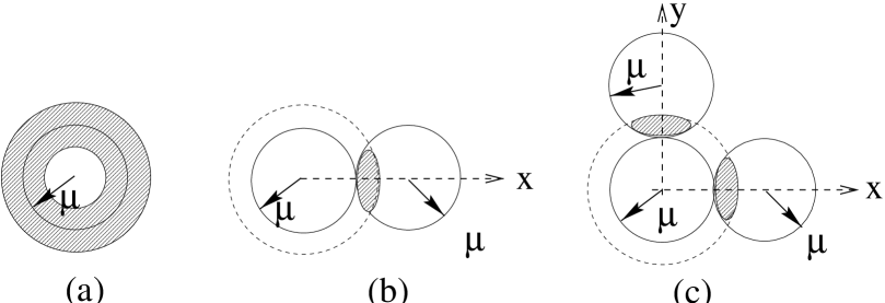
Figure 1: (a) fraction of the Fermi surface used in BCS pairing; (b) fraction of the Fermi surface used in the Overhauser pairing with one standing wave; (c) fractions of the Fermi surface used in the Overhauser pairing with two orthogonal standing waves.

5. Screened Case: Finite $N_{c}$

In the presence of electric and magnetic screening, which are important in matter, the situation changes significantly. While the original variational arguments in [4] were tailored for the unscreened case, our formulation which reproduces exactly their unscreened results in the leading logarithm approximation, generalizes naturally to the screened perturbative and nonperturbative cases in a minimal way. Indeed, using (28-29) and the pertinent transverse cutoffs, we obtain for perturbative screening,

$$F(p_{||}) \!\!\approx\!\! \frac{h^{2}}{6}\int_{0}^{\infty}\!dq_{||}\,\frac{F(q_{||})}{\sqrt{q_{||}^{2}+F^{2}(q_{||})}}$$

$$\qquad\mbox{}\times\,\ln\left\{\left(1+\frac{\Lambda_{\perp}^{2}}{(p_{||}\mbox{$-$}q_{||})^{2}+m_{E}^{2}}\right)^{3}\left(1+\frac{\Lambda_{\perp}^{3}}{|p_{||}\mbox{$-$}q_{||}|^{3}+\frac{\pi}{4}m_{D}^{2}|p_{||}\mbox{$-$}q_{||}|}\right)^{2}\,\right\},$$

$$G(p_{||}) \!\!\approx\!\! \frac{h^{2}_{\ast}}{6}\int_{0}^{\infty}\!dq_{||}\,\frac{G(q_{||})}{\sqrt{q_{||}^{2}+|G(q_{||})|^{2}}}$$

$$\qquad\mbox{}\times\,\ln\left\{\left(1+\frac{\Lambda_{\perp}^{2}}{(p_{||}\mbox{$-$}q_{||})^{2}+m_{E}^{2}}\right)^{3}\left(1+\frac{\Lambda_{\perp}^{3}}{|p_{||}\mbox{$-$}q_{||}|^{3}+\frac{\pi}{4}m_{D}^{2}|p_{||}\mbox{$-$}q_{||}|}\right)^{2}\,\right\},$$

and for nonperturbative screening

$$F(p_{||}) \approx h^{2}\int_{0}^{\infty}dq_{||}\,\frac{F(q_{||})}{\sqrt{q_{||}^{2}+F^{2}(q_{||})}}\,\ln\left|1+\frac{\Lambda_{\perp}^{2}}{(p_{||}-q_{||})^{2}+im_{*}^{2}}\right|\;,$$

$$G(p_{||}) \approx h_{\ast}^{2}\int_{0}^{\infty}dq_{||}\,\frac{G(q_{||})}{\sqrt{q_{||}^{2}+|G(q_{||})|^{2}}}\,\ln\left|1+\frac{\Lambda_{\perp}^{2}}{(p_{||}-q_{||})^{2}+im_{*}^{2}}\right|$$

where the transverse cutoffs are $\Lambda_{\perp}=\sqrt{2\mu\epsilon_{q}}$ (Overhauser) and $\Lambda_{\perp}=2\mu$ (BCS) respectively. The cutoffs are exactly fixed in weak coupling, and reflect on the fractions of the Fermi surface used in the pairing.

In the BCS case, the transverse cutoff is large. Hence $\Lambda_{\perp}>m_{E},m_{M}$ and the logarithm in (LABEL:S27) may not be expanded. Dropping 1, we obtain to leading logarithm accuracy,

$$G_{0}\approx\left(\frac{4\Lambda_{\perp}^{6}}{\pi m_{E}^{5}}\right)\,e^{-\frac{\sqrt{3}\pi}{2h_{\ast}}}\;.$$ (46)

The results for the BCS gap is the same as the one reached in [20, 19, 18]  if we were to Fierz with ${\bf M}_{B}$ instead of ${\bf M}_{C}$. Note that (46) is smaller than (42) as expected. For nonperturbative screening, the result is

$$G_{0}\approx\Lambda_{\perp}e^{-\frac{2}{h_{\ast}^{2}}\left\{\ln(1+\Lambda_{\perp}^{4}/m_{*}^{4})\right\}^{-1}}$$ (47)

with $\Lambda_{\perp}/m_{*}=2\mu/m_{*}\gg 1$.

In the Overhauser case, the transverse cutoff is reduced in comparison to the BCS case due to momentum conservation for fixed 3-momentum for the standing wave. The equation can be rearranged into the form

$$F(p_{||}) \approx \frac{h^{2}}{6}\int_{0}^{\infty}dq_{||}\,\frac{F(q_{||})}{\epsilon_{q}}\,{\rm ln}\left(\frac{2\mu\epsilon_{q}}{(p_{||}-q_{||})^{2}}\right)$$ (48)

$$\mbox{}+\frac{5h^{2}}{6}\int_{0}^{\infty}dq_{||}\,\frac{F(q_{||})}{\epsilon_{q}}\,{\rm ln}\left(\frac{2\mu\epsilon_{q}}{(p_{||}-q_{||})^{2}+m_{E}^{2}}\right)\,,$$

where we have approximated $\pi m_{D}^{2}/4\sim m_{E}^{2}$ and used static, but perturbatively screened propagators. The effects of Landau damping through the magnetic gluons result into an unscreened interaction but with a reduced strength $h^{2}\rightarrow h^{2}/6$. Eq. (48) can be solved to leading logarithm accuracy using the logarithmic scales as defined above. Specifically, for $x<x_{m}\equiv\ln(2\mu/m_{E})$, we get

$$F(x)\approx h^{2}\left(2x\int_{x}^{x_{L}}dy\,F(y)-\int_{x}^{x_{L}}dy\,yF(y)+\int_{0}^{x}dy\,yF(y)\right)$$ (49)

as in the unscreened case with $x_{L}=x_{0}$, and for $x>x_{m}$

$$F(x)\approx\frac{h^{2}}{6}\left(2x\int_{x}^{x_{R}}dy\,F(y)-\int_{x}^{x_{R}}dy\,yF(y)+\int_{0}^{x}dy\,yF(y)\right)+{\cal C}\;.$$ (50)

Here $x_{L,R}\equiv\ln(2\mu/F_{L,R})$ and the constant ${\cal C}$ is given by

$${\cal C}=\frac{5h^{2}}{6}\int_{0}^{\infty}dq_{||}\,\frac{F(q_{||})}{\epsilon_{q}}\,{\rm ln}\left(\frac{2\mu\epsilon_{q}}{{\rm max}\,(q_{||}^{2},m_{E}^{2})}\right)\;.$$ (51)

The solution to (49-50) is

$$\begin{array}[]{lclclcl}F(x)&=&F_{L}\cos(\sqrt{2}\,h\,(x-x_{L}))&\qquad\mbox{for}&x&<&x_{m}\;,\\ F(x)&=&F_{R}\cos(h\,(x-x_{R})/\sqrt{3})&\qquad\mbox{for}&x&>&x_{m}\;.\end{array}$$

We note that for $x<x_{m}$ or $p_{||}>m_{E}$, screening can be ignored to leading logarithm accuracy and $x_{L}=\pi/\sqrt{2}h$ as before. For $x>x_{m}$ or $p_{||}<m_{E}$, screening cannot be ignored to leading logarithm accuracy. Continuity at $x_{m}$ fixes $x_{R}$, so that

$$F_{R}=F_{L}\,\,\frac{\cos\left\{\sqrt{2}\,h\,(x_{m}-x_{L})\right\}}{\cos\left\{h\,(x_{m}-x_{R})/\sqrt{3}\right\}}=e^{-\pi/\sqrt{2}h}\frac{\cos\left\{\sqrt{2}\,h\ln\left(\frac{2\mu}{m_{E}}\right)-\pi\right\}}{\cos\left\{h\left[\ln\left(\frac{2\mu}{m_{E}}\right)-\ln\left(\frac{2\mu}{F_{R}}\right)\right]/\sqrt{3}\right\}}\;.$$ (52)

Eq. (52) defines a transcendental equation for $F_{R}/2\mu$ as a function of $N_{f},N_{c}$ and $h$ (equivalently $\mu$), i.e.

$$\frac{F_{R}}{2\mu}\approx-{e^{-\pi/\sqrt{2}h}}\,\,\frac{\cos\left\{\frac{h}{\sqrt{2}}\ln\left(\frac{N_{c}}{N_{f}h^{2}}\right)\right\}}{\cos\left\{\frac{h}{\sqrt{3}}\ln\left(\sqrt{\frac{N_{c}}{N_{f}h^{2}}}\frac{F_{R}}{2\mu}\right)\right\}}\;\;,$$ (53)

where we have used $m_{E}/2\mu\approx h\,\sqrt{N_{f}/N_{c}}\,\,$, with

$$\frac{1}{h^{2}}\approx\frac{8\pi^{2}}{N_{c}g^{2}}\approx\frac{11}{3}\,{\rm ln}\,\left(\frac{\mu}{\Lambda_{QCD}}\right)+\frac{17}{11}\,{\rm ln}\,{\rm ln}\,\left(\frac{\mu}{\Lambda_{QCD}}\right)$$ (54)

to two loops. For fixed $N_{c}$ and in weak coupling ($h\rightarrow 0$), there is no solution to (53) as can be seen by inspection. This corresponds to a screening mass with power suppression, e.g. $m_{E}/\mu\approx h$. However, a solution can be found in weak coupling but large $N_{c}$, when approximatly

$$e^{-\pi/\sqrt{2}h}\,\sqrt{\frac{N_{c}}{N_{f}h^{2}}}\approx 1$$ (55)

for which $F_{R}\approx F_{L}$. Through $N_{c}$, this corresponds to a screening mass with exponential suppression, e.g. $m_{E}/\mu\approx e^{-\pi/\sqrt{2}h}$.

To assess the minimal value of $N_{c}$ for which there is a solution to (53), it is useful to note that the solution (S0.Ex22) is invariant under the shift

$$x\rightarrow x+\ln\left(\frac{\Lambda_{\perp}}{2\mu}\right)$$ (56)

with similar shifts in the scales $x_{m,L,R}$, implying the existence of a family of solutions that depend parametrically on $x_{m,L,R}$ and $\Lambda_{\perp}$. The harmonic equation satisfied by $F(x)$ is scale invariant, hence of the renormalization group type . The scale $x_{R}$ is fixed in terms of $x_{L,m}$ by demanding that the logarithmic derivatives of (S0.Ex22) (with pertinent shifts) match at $x_{m}$. Thus

$$\frac{1}{\sqrt{6}}\tan\left(\frac{h}{\sqrt{3}}\,(x_{m}-x_{R})\right)=\tan\left(\sqrt{2}h\,(x_{m}-x_{L})\right)\;,$$ (57)

with

$$x_{R}=-\frac{\sqrt{3}}{h}\,\left\{\arctan\left[\sqrt{6}\,\tan\left(\sqrt{2}h\,(x_{m}-x_{L})\right)\right]+{\rm mod}\,\pi\right\}+x_{m}\;.$$ (58)

The lower bound on $N_{c}$ or equivalently the upper bound on the electric mass follows from

$$m_{E}\equiv\Lambda_{\perp}\,e^{-x_{m}}=\left(\frac{\Lambda_{\perp}^{2}}{2\mu}\right)\left(\frac{2\mu}{\Lambda_{\perp}}\right)\,e^{-x_{m}}\leq 2\mu\left(\frac{\Lambda_{||}}{\Lambda_{\perp}}\right)\,e^{-x_{m}}\equiv 2\mu\,e^{-x_{||}-x_{m}}\,\,,$$ (59)

where $\Lambda_{\perp}$ and $\Lambda_{||}$ are now exponentially small scales characterizing the spread in $p_{\perp}$ and $p_{||}$. The inequality in (59) follows from the geometrical constraint $\Lambda_{||}\geq\Lambda_{\perp}^{2}/2\mu$ discussed above (see (32) and also Fig. 1b). Up to the rescaling (56), the maximum $\Lambda_{||}$ for which there is a solution (S0.Ex22) with positive semi-definite gap, corresponds to $F(x_{||})=0$, i.e. $x_{||}=x_{R}+\sqrt{3}\pi/2h$. (The alternative solution $x_{||}=x_{L}+\sqrt{2}\pi/4h$ does not generate a maximum bound.) After inserting the latter and (58) into $\hat{c}\equiv\sqrt{2}\,h\,{\rm min}\,(x_{||}+x_{m})$, we determine the minimum as $\hat{c}\approx 2.5051$ and the lower bound for $N_{c}$ (upper bound for the electric mass $m_{E}$) as

$$\frac{N_{c}}{N_{f}}\geq h^{2}\,e^{\sqrt{2}\hat{c}/h}\;.$$ (60)

This result is in overall agreement with a recent renormalization group estimate [5] . In particular, for $\mu=3\Lambda_{QCD}$, we find $N_{c}\geq 334\,N_{f}$.

The case of nonperturbative screening can be addressed similarly by noting that (48) is now

$$F(p_{||})\approx\frac{h^{2}}{2}\int_{0}^{\infty}\,dq_{||}\,\frac{F(q_{||})}{\epsilon_{q}}\,{\rm ln}\left(\frac{(2\mu\epsilon_{q})^{2}}{(p_{||}-q_{||})^{4}+m_{*}^{4}}\right)\;.$$ (61)

For $x<x_{m}$ or $p_{||}>m_{*}$ the screening in (61) is inactive. Hence $F(x)=-F_{L}{\rm cos}(\sqrt{2}hx)$, while for $x>x_{m}$ or $p_{||}<m_{*}$ the screening overwhelms the leading logarithm accuracy with $F(x)={\rm const}$. Continuity at $x_{m}$ requires that $x_{m}=x_{L}$. Hence

$$m_{*}=2\mu\,e^{-\frac{\pi}{\sqrt{2}h}}$$ (62)

which is the maximum tolerated nonperturbative screening mass for an Overhauser pairing to take place.

Finally, we can qualitatively analyze the effects of temperature on the Overhauser effect by considering the distribution of quasiparticles at the Fermi surface. At finite temperature $T$, the pairing energy becomes

$$F(p_{||}) \approx \frac{h^{2}}{6}\int_{0}^{\infty}dq_{||}\,\frac{F(q_{||})}{\epsilon_{q}}\,{\rm ln}\left(\frac{2\mu\epsilon_{q}}{(p_{||}-q_{||})^{2}}\right)\,{\rm tanh}\left(\frac{\epsilon_{q}}{2T}\right)$$ (63)

$$\mbox{}+\frac{5h^{2}}{6}\int_{0}^{\infty}dq_{||}\,\frac{F(q_{||})}{\epsilon_{q}}\,{\rm ln}\left(\frac{2\mu\epsilon_{q}}{(p_{||}-q_{||})^{2}+m_{E}(T)^{2}}\right)\,{\rm tanh}\left(\frac{\epsilon_{q}}{2T}\right)\,,$$

with the temperature dependent screening mass [15]

$$m^{2}_{E}(T)=m_{E}^{2}+\left(N_{c}+\frac{N_{f}}{2}\right)\,\frac{g^{2}T^{2}}{3}\,.$$ (64)

Even at large $N_{c}$ the screening mass is finite. We conclude that at finite temperature, the Overhauser pairing is rapidly depleted by screening for any value of $N_{c}$.

6. Pairing in Lower Dimensions

The results we have derived depend on the number of dimensions. Indeed, the QCD analysis we have carried out when applied to 1+1 dimensions yield the following energy gaps

$$F(p) \approx h^{2}\int_{0}^{\infty}dq\,\frac{F(q)}{\epsilon_{q}}\,\,\,\frac{1}{(p-q)^{2}+m_{E}^{2}}\;,$$

$$G(p) \approx h_{*}^{2}\int_{0}^{\infty}dq\,\frac{G(p)}{\epsilon_{q}}\,\,\,\frac{1}{(p-q)^{2}+m_{E}^{2}}\;,$$ (65)

with the replacement $g^{2}/8\pi^{2}\rightarrow g^{2}/2\pi$ in $h^{2}$ and $h^{2}_{*}$. Remember that $F(q)$ and $G(q)$ have been defined as even functions. In deriving (65) we have followed the same logic as in 3+1 dimensions, thereby ignoring self-energy insertion on the quark line, and the gauge-fixing dependence on the gluon propagator. While these two effects cancel in color singlet states (Overhauser) [26], they usually do not in color-non-singlet states (BCS) except for the case of $N_{c}=2$ [22]. In 1+1 dimensions $g^{2}/2\pi$ has mass dimension, and there is only electric screening with $m_{E}^{2}\approx N_{f}g^{2}\,{\rm ln}\,(\mu/g)$. Clearly,

$$F_{0}\approx\Lambda\,e^{-{m_{E}^{2}}/{h^{2}}}\gg G_{0}\approx\Lambda\,e^{-{m_{E}^{2}}/{h_{*}^{2}}}\,\,.$$ (66)

The dominance of the Overhauser effect over the BCS effect whatever $N_{c}$, stems from the fact that the Fermi surface reduces to 2 points ($\pm\mu$) in 1+1 dimensions, with no phase space reduction for the former. Since both the Overhauser and BCS phase break spontaneously chiral symmetry at finite density, the existence of the Overhauser phase may rely ultimatly on large $N_{c}$. The Overhauser effect is dominant in the Schwinger model where $G_{0}=0$ because of the repulsive character of the Coulomb interaction , confirming the results in [7, 8, 9]. The case of QCD in 2+1 dimensions will be discussed elsewhere.

7. Conclusions

We have constructed a Wilsonian effective action for various scalar-isoscalar excitations around the Fermi surface. Our analysis in the decoupled mode shows that in weak-coupling, the Overhauser effect can overtake the BCS effect only at large $N_{c}$ in the scalar-isoscalar channel, in agreement with a recent renormalization group result [5]. The BCS pairing is more robust to screening than the Overhauser pairing in weak coupling. The BCS analysis was carried out for both the CFL and the antisymmetric arrangements for arbitrary $N_{c}\geq 3$, $N_{f}\geq 2$, ignoring the superconducting penetration lengths since the electric and magnetic screening lengths are smaller than the London and Pippard lengths (for type-I superconductors). In strong coupling, the Overhauser effect appears to be comparable to the BCS effect, especially if multiple standing waves are used, allowing for further cooperative pairing between adjacent patches. This is particularly relevant for pairings with large energy gaps which are expected to take place at a few times nuclear matter density [19].

Our effective action is better suited to the use of variational approximations as discussed in [4], and leads naturally to exact integral equations by variations, especially in the presence of interactions with retardation and screening. It would be interesting to repeat our analysis at nonasymptotic densities using instanton-generated vertices to address the Overhauser effect. Indeed, for instantons the cutoff is fixed from the onset by their inverse size. As we have shown here, the Overhauser pairing, much like the BCS pairing by magnetic forces [20], relies on scattering between pairs in the forward direction that is kinematically suppressed in the transverse directions (in fact exponentially suppressed [4]). Since the instanton interaction is nearly uniform over the Fermi sphere, we expect a geometrical enhancement in the BCS pairing in comparison to the Overhauser pairing. We recall that in the latter the interaction is enhanced by a factor of order $N_{c}$. Which one dominates at a few times nuclear matter density and $N_{c}=3$ is not clear a priori. Instantons in the vacuum crystallize for $N_{c}\geq 20$ [27] in the quenched approximation, and $3<N_{c}<20$ in the unquenched case. The crystallization is likely to be favored by finite $\mu$ as the quarks are forced to line-up along the forward $x_{4}$-direction.

It is amusing to note that the crystal phase breaks color, flavor, and translational symmetry spontaneously, with the occurrence of color and flavor density waves. In many ways, this situation resembles the one encountered with dense Skyrmions [10] (strong coupling), suggesting the possibility of a smooth transition. In the process, color and flavor, respectively, may get misaligned [28], resulting into color-flavor-locked charge density waves in a normal (large gaps) phase. The Skyrmion crystal at low density may smoothly transmute to a qualiton crystal at intermediate densities, with crystalline structure commensurate with the number of patches on the Fermi surface. We note that the crystalline structure in $3+1$ dimensions may only show up as rapid variations in the response functions at momentum $2\mu$. This is not the case in 1+1 and 2+1 dimensions [3].

Although we have carried out the analysis using Feynman gauge with minimal changes for the electric and magnetic screening, we expect our estimates of the gap energies to be reliable since a close inspection of the equations we derived when reinterpreted in Minkowski space, shows that the quoted results originate from the forward scattering amplitude of quarks around the Fermi surface. The latter is infrared sensitive in the unscreened case and gauge independent, the exception being in 1+1 dimension [26, 22]. The similarity between forward particle-particle and particle-hole scattering resembles the similarity between forward Compton and Bhabha scattering. This is what makes $2\mu$ and opposite sides to the Fermi surface so special between a particle and a hole.

Finally, it is amusing to note that following either the Overhauser or BCS pairing, the quark eigenvalues of the QCD Dirac operator would suggest a novel rearrangement that is characterized by novel spectral sum rules. They will be reported elsewhere. Our use of the effective action at the Fermi surface is more than a convenience for the study of QCD at large quark chemical potential. Indeed, given the shortcomings faced by important samplings in lattice Monte Carlo simulations at finite quark chemical potential, and also given the importance of Pauli blocking for the non-surface modes, we believe that a convenient formulation of QCD on the lattice should make use of Fermionic fields projected onto the Fermi surface, much like the ones used in the present work, and in the spirit of the heavy-quark formalism [14].

References

• [1] D. Bailin and A. Love, Phys. Rept. 107, 325 (1984).
• [2] M. Alford, K. Rajagopal and F. Wilczek, Phys. Lett. B422, 247 (1998), hep-ph/9711395; R. Rapp, T. Schäfer, E.V. Shuryak and M. Velkovsky, Phys. Rev. Lett. 81, 53 (1998), hep-ph/9711396; T. Schäfer, Nucl. Phys. A638, 511C (1998); M. Alford, K. Rajagopal and F. Wilczek, Nucl. Phys. A638, 515C (1998), hep-ph/9802284; K. Rajagopal, Prog. Theor. Phys. Suppl. 131, 619 (1998), hep-ph/9803341; J. Berges and K. Rajagopal, Nucl. Phys. B538, 215 (1999), hep-ph/9804233; M. Alford, K. Rajagopal and F. Wilczek, Nucl. Phys. B537, 443 (1999), hep-ph/9804403; T. Schäfer, Nucl. Phys. A642, 45 (1998), nucl-th/9806064; S. Hands and S.E. Morrison [UKQCD Collaboration], Phys. Rev. D59, 116002 (1999), hep-lat/9807033; K. Rajagopal, Nucl. Phys. A642, 26 (1998), hep-ph/9807318; N. Evans, S.D.H. Hsu and M. Schwetz, Nucl. Phys. B551, 275 (1999), hep-ph/9808444; S. Morrison [UKQCD Collaboration], Nucl. Phys. Proc. Suppl. 73, 480 (1999), hep-lat/9809040; T. Schäfer and F. Wilczek, Phys. Lett. B450, 325 (1999), hep-ph/9810509; N. Evans, S.D.H. Hsu and M. Schwetz, Phys. Lett. B449, 281 (1999), hep-ph/9810514; R.D. Pisarski and D.H. Rischke, Phys. Rev. Lett. 83, 37 (1999), nucl-th/9811104; K. Langfeld and M. Rho, hep-ph/9811227; T. Schäfer and F. Wilczek, Phys. Rev. Lett. 82, 3956 (1999), hep-ph/9811473; D.T. Son, Phys. Rev. D59, 094019 (1999), hep-ph/9812287; A. Chodos, H. Minakata and F. Cooper, Phys. Lett. B449, 260 (1999), hep-ph/9812305; J. Hosek, hep-ph/9812515; G.W. Carter and D. Diakonov, Phys. Rev. D60, 016004 (1999), hep-ph/9812445; D.K. Hong, hep-ph/9812510; S. Hands and S. Morrison, hep-lat/9902011; N.O. Agasian, B.O. Kerbikov and V.I. Shevchenko, hep-ph/9902335; R.D. Pisarski and D.H. Rischke, nucl-th/9903023; T.M. Schwarz, S.P. Klevansky and G. Papp, nucl-th/9903048; M. Alford, J. Berges and K. Rajagopal, hep-ph/9903502; T. Schäfer and F. Wilczek, Phys. Rev. D60, 074014 (1999), hep-ph/9903503; R. Rapp, T. Schäfer, E.V. Shuryak and M. Velkovsky, hep-ph/9904353; D. Blaschke, D.M. Sedrakian and K.M. Shahabasian, astro-ph/9904395; S. Hands and S. Morrison, hep-lat/9905021; G.W. Carter and D. Diakonov, hep-ph/9905465; E. Shuster and D.T. Son, hep-ph/9905448; A. Chodos, F. Cooper and H. Minakata, hep-ph/9905521; D.K. Hong, hep-ph/9905523; R.D. Pisarski and D.H. Rischke, nucl-th/9906050; D.K. Hong, V.A. Miransky, I.A. Shovkovy and L.C. Wijewardhana, hep-ph/9906478; T. Schäfer and F. Wilczek, hep-ph/9906512; D.K. Hong, M. Rho and I. Zahed, hep-ph/9906551; M. Rho, nucl-th/9908015; R. Casalbuoni and R. Gatto, hep-ph/9908227; M. Alford, J. Berges and K. Rajagopal, hep-ph/9908235; W.E. Brown, J.T. Liu and H. Ren, hep-ph/9908248; E.V. Shuryak, hep-ph/9908290; S.D.H. Hsu and M. Schwetz, hep-ph/9908310; G.W. Carter and D. Diakonov, hep-ph/9908314; D. Blaschke, T. Klahn and D.N. Voskresensky, astro-ph/9908334; F. Wilczek, hep-ph/9908480; T. Schäfer, nucl-th/9909013; A. Chodos, F. Cooper, W. Mao, H. Minakata and A. Singh, hep-ph/9909296; R. Casalbuoni and R. Gatto, hep-ph/9909419; T. Schäfer, hep-ph/9909574; P.F. Bedaque, hep-ph/9910247; M. Alford, J. Berges and K. Rajagopal, hep-ph/9910254; B. Vanderheyden and A.D. Jackson, hep-ph/9910295; N. Evans, J. Hormuzdiar, S.D.H. Hsu, M. Schwetz, hep-ph/9910313.
• [3] A.W. Overhauser, Advances in Physics 27, 343-363 (1978).
• [4] D.V. Deryagin, D.Y. Grigorev and V.A. Rubakov, Int. J. Mod. Phys. A7, 659-681 (1992).
• [5] E. Shuster and D.T. Son, hep-ph/9905448.
• [6] J. Schwinger, Phys. Rev. 128, 2425 (1962).
• [7] W. Fischler, J. Kogut and L. Susskind, Phys. Rev. D 19, 1188-1197 (1979).
• [8] H.R. Christiansen and F.A. Schaposnik, Phys. Rev. D 53, 3260-3265 (1996); Phys. Rev. D 55, 4920-4930 (1997).
• [9] Y.C. Kao and Y.W. Lee, Phys. Rev. D 50 1165-1166 (1994).
• [10] I. Klebanov, Nucl. Phys. B262, 133 (1985); L. Castillejo, P.S. Jones, A.D. Jackson, J.J. Verbaarschot and A. Jackson, Nucl. Phys. A501, 801 (1989); H. Forkel, A.D. Jackson, M. Rho, C. Weiss, A. Wirzba and H. Bang, Nucl. Phys. A504, 818 (1989).
• [11] A.S. Goldhaber and N.S. Manton, Phys. Lett. 198B, 231 (1987); N.S. Manton and P.M. Sutcliffe, Phys. Lett. B342, 196 (1995), hep-th/9409182.
• [12] T.D. Cohen, Nucl. Phys. A495, 545 (1989).
• [13] M.A. Nowak, M. Rho and I. Zahed, Chiral nuclear dynamics  (World Scientific, Singapore, 1996).
• [14] M. Rho, A. Wirzba and I. Zahed, in preparation.
• [15] M. Le Bellac, Thermal Field Theory  (Cambridge University Press, Cambridge 1996).
• [16] I. Zahed and D. Zwanziger, hep-th/9905109; Phys. Rev. D in print.
• [17] R.T. Cahill and S.M. Gunner, Fizika B7, 171-202 (1998), hep-ph/9812491.
• [18] R.D. Pisarski and D.H. Rischke, nucl-th/9907041.
• [19] T. Schäfer and F. Wilczek, hep-ph/9906512.
• [20] D.T. Son, Phys. Rev. D59, 094019 (1999), hep-ph/9812287.
• [21] T. Schäfer, hep-ph/9909574.
• [22] V.N. Pervushin and D. Ebert, Teor. Mat. Fiz. 36, 313-323 (1978); D. Ebert and L. Kaschluhn, Nucl. Phys. B355, 123-132 (1991).
• [23] K. Langfeld and M. Rho, hep-ph/9811227.
• [24] R.D. Pisarski and D.H. Rischke, nucl-th/9907094.
• [25] B.-Y. Park, M. Rho, A. Wirzba and I. Zahed, in preparation.
• [26] G. ’t Hooft, Nucl. Phys. B72, 461 (1974); Nucl. Phys. B75, 461 (1974).
• [27] D.I. Diakonov and V.Y. Petrov, Nucl. Phys. B245, 259 (1984).
• [28] D.B. Kaplan, Phys. Lett. B235, 163 (1990); Nucl. Phys. B351, 137 (1991).