PHENOMENOLOGY OF
NEUTRINO MASSES AND MIXING

Abstract

We discuss all possible schemes with four massive neutrinos inspired by the existing experimental indications in favour of neutrino mixing, namely the atmospheric, solar and LSND neutrino experiments. We argue that the scheme with a neutrino mass hierarchy is not compatible with the experimental results, likewise all other schemes with the masses of three neutrinos close together and the fourth mass separated by a gap needed to incorporate the LSND neutrino oscillation result. Only two schemes with two pairs of neutrinos with nearly degenerate masses separated by this gap of the order of 1 eV are in agreement with the results of all experiments, including those where no indications for neutrino oscillations have been found. We also point out the possible effect of big-bang nucleosynthesis on the 4-neutrino mixing matrix and its consequences for neutrino oscillations. Finally, we study predictions for neutrino oscillation experiments and ³H and $(\beta\beta)_{0\nu}$ decays, following from the two favoured neutrino mass spectra and mixing schemes. These predictions can be conceived as checks of the input used for arriving at the two favoured schemes.

The scope of this article

At present there are three indications in favour of neutrino oscillations: the results of the solar [1, 2, 3, 4, 5], atmospheric [6, 7, 8, 9, 10, 11, 12, 13] and LSND experiments [14, 15, 16]. These three indications require three different scales of mass-squared differences and, therefore, four neutrinos with definite mass. Since the LEP experiments [17] have shown that the number of active neutrinos is three, a fourth neutrino is needed which is sterile, i.e., its couplings to the $W$ and $Z$ bosons are zero or negligible.

In this paper we take all three indications seriously and thus discuss the phenomenological analysis of all existing neutrino data in terms of

3 active + 1 sterile neutrino.

We will consider the topics of the nature of the possible neutrino mass spectra, constraints on the neutrino mixing matrix from the oscillation data and from big-bang nucleosynthesis, and finally checks and consequences ensuing from the favoured neutrino mass spectra and the associated mixing matrices.

In the following we will use the abbreviations SBL for short-baseline, LBL for long-baseline and BBN for big-bang nucleosynthesis.

I Introduction

A Neutrino mixing

Neutrino masses and neutrino mixing are natural phenomena in gauge theories extending the Standard Model (see, for example, Ref. [18]). However, for the time being, masses and mixing angles cannot be predicted on theoretical grounds and they are the central subject of the experimental activity in the field of neutrino physics.

In the general discussion, we assume that there are $n$ neutrino fields with definite flavours and that neutrino mixing is described by a $n\times n$ unitary mixing matrix $U$ [19] such that

$$\nu_{{\alpha}L}=\sum_{j=1}^{n}U_{{\alpha}j}\,\nu_{jL}\qquad(\alpha=e,\mu,\tau,s_{1},\dots,s_{n-3})\,.$$ (1)

Note that the neutrino fields $\nu_{\alpha L}$ other than the three active neutrino flavour fields $\nu_{eL}$, $\nu_{\mu L}$, $\nu_{\tau L}$ must be sterile (for a review see Ref. [20]) to comply with the result of the LEP measurements of the number of neutrino flavours. The fields $\nu_{jL}$ ($j=1,\dots,n$) are the left-handed components of neutrino fields with definite masses $m_{j}$. We assume the ordering $m_{1}\leq m_{2}\leq\ldots\leq m_{n}$ for the neutrino masses.

The most striking feature of neutrino masses and mixing is the quantum-mechanical effect of neutrino oscillations [21] (for a review on the early years of neutrino oscillations see Ref. [22]). The transition ($\alpha\neq\beta$) or survival ($\alpha=\beta$) probability for $\nu_{\alpha}\rightarrow\nu_{\beta}$ is given by

$$P_{\nu_{\alpha}\rightarrow\nu_{\beta}}=\left|\sum_{j=1}^{n}U_{\beta j}U_{\alpha j}^{*}\exp\!\left(-i\frac{\Delta{m}^{2}_{j1}L}{2E}\right)\right|^{2}\,,$$ (2)

where $\Delta{m}^{2}_{jk}\equiv m^{2}_{j}-m^{2}_{k}$, $L$ is the distance between neutrino source and detector and $E$ is the neutrino energy. Eq.(2) is valid for ultrarelativistic neutrinos with $m^{2}_{j}/E^{2}\ll 1$ ($j=1,\ldots,n$). There are additional conditions depending on the neutrino production and detection processes which must hold for the validity of Eq.(2). See, e.g., Ref. [23] and references therein.

Let us indicate some important features of Eq.(2):

• The oscillation probability $P_{\bar{\nu}_{\alpha}\rightarrow\bar{\nu}_{\beta}}$ for antineutrinos is obtained from $P_{\nu_{\alpha}\rightarrow\nu_{\beta}}$ by making the replacement $U\to U^{*}$.

• The probabilities $P_{\nu_{\alpha}\rightarrow\nu_{\beta}}$ and $P_{\bar{\nu}_{\alpha}\rightarrow\bar{\nu}_{\beta}}$ depend only on mass-squared differences, which is explicitly shown by the phase factor $\exp(im^{2}_{1}L/2E)$ multiplying the expression within the absolute value in the probability (2).

• The oscillation probabilities $P_{\nu_{\alpha}\rightarrow\nu_{\beta}}$ and $P_{\bar{\nu}_{\alpha}\rightarrow\bar{\nu}_{\beta}}$ do not distinguish between the Dirac or Majorana nature of neutrinos. Note that neutrino fields of different natures cannot mix.

• In the oscillation probabilities, phases of the form

  $$\frac{\Delta m^{2}L}{2E}\simeq 2.53\times\left(\frac{\Delta m^{2}}{1\,\mbox{eV}^{2}}\right)\left(\frac{E}{1\,\mbox{MeV}}\right)^{-1}\left(\frac{L}{1\,\mbox{m}}\right)$$ (3)

  occur, where $\Delta m^{2}$ is a generic mass-squared difference. Given $E$ and $L$, these phases determine the order of magnitude of $\Delta m^{2}$ a neutrino oscillation experiment is sensitive to.

Let us discuss two examples illustrating the last point. Clearly, experiments can only see phases (3) if they are not too small, say if they are of order 1. The first example concerns SBL reactor experiments. By convention, SBL experiments are sensitive to mass-squared differences $\Delta m^{2}\gtrsim 0.1$ eV². With $E\sim 1$ MeV it follows that $L\gtrsim 10$ m is a sufficient distance between neutrino source and detector to achieve this sensitivity. On the other hand, the longest baseline possible on earth is 13000 km, the diameter of the earth. In this case, the atmospheric neutrino flux is available with the largest flux around $E\sim 1$ GeV. The requirement that the phase (3) is larger than 0.1 leads to a sensitivity estimate of $\Delta m^{2}\gtrsim 10^{-4}$ eV².

B Indications in favour of neutrino oscillations

At present, indications that neutrinos are massive and mixed have been found in solar neutrino experiments (Homestake [1], Kamiokande [2], GALLEX [3], SAGE [4] and Super-Kamiokande [5]), in atmospheric neutrino experiments (Kamiokande [6], IMB [7], Soudan [8], Super-Kamiokande [9] and MACRO [13]) and in the LSND experiment [14, 15] (see also the review [24]). From the analyses of the data of these experiments in terms of neutrino oscillations one infers the following scales of neutrino mass-squared differences:

• Solar neutrino deficit: Interpreted as effect of neutrino oscillations, the relevant value of the mass-squared difference is determined as [25, 26]

  $$\Delta{m}^{2}_{\mathrm{solar}}\sim 10^{-5}\,\mathrm{eV}^{2}\,(\mbox{MSW})\quad\mbox{or}\quad\Delta{m}^{2}_{\mathrm{solar}}\sim 10^{-10}\,\mathrm{eV}^{2}\,(\mbox{vac. osc.})$$ (4)

  The two possibilities for $\Delta{m}^{2}_{\mathrm{solar}}$ correspond, respectively, to the MSW [27] and to the vacuum oscillation solutions of the solar neutrino problem. The solar neutrino experiments are $\nu_{e}$ disappearance experiments.

• Atmospheric neutrino anomaly: Interpreted as effect of neutrino oscillations, the zenith angle dependence of the atmospheric neutrino anomaly [6, 9] using the so-called contained and partially contained multi-GeV events [12] gives

  $$\Delta{m}^{2}_{\mathrm{atm}}=3.5\times 10^{-3}\,\mathrm{eV}^{2}$$ (5)

  with $\sin^{2}2\theta_{\mathrm{atm}}=1$ for the mixing angle as best fit values under the assumption of $\stackrel{{\scriptstyle\scriptscriptstyle(-)}}{{\nu}}_{\hskip-3.0pt\mu}\to\stackrel{{\scriptstyle\scriptscriptstyle(-)}}{{\nu}}_{\hskip-3.0pt\tau}$ oscillations. In essence, the atmospheric neutrino anomaly is interpreted as $\stackrel{{\scriptstyle\scriptscriptstyle(-)}}{{\nu}}_{\hskip-3.0pt\mu}$ disappearance.

• LSND experiment: The evidence for $\stackrel{{\scriptstyle\scriptscriptstyle(-)}}{{\nu}}_{\hskip-3.0pt\mu}\to\stackrel{{\scriptstyle\scriptscriptstyle(-)}}{{\nu}}_{\hskip-3.0pte}$ oscillations in this experiment leads to [14]

  $$\Delta{m}^{2}_{\mathrm{LSND}}\sim 1\,\mathrm{eV}^{2}\,.$$ (6)

  The result of the LSND experiment is the only evidence for neutrino appearance.

Thus, due to the three different scales of $\Delta m^{2}$, at least four light neutrinos with definite masses must exist in nature in order to accommodate the results of all neutrino oscillation experiments, and because of the LEP result on the number of active neutrinos the existence of at least one non-interacting sterile neutrino is required. In the following, apart from the SBL discussion in Section III, we will confine ourselves to four neutrinos. For early works on four neutrinos see Ref. [28], for general phenomenological discussions see Refs. [29, 30, 31, 32].

II Types of 4-neutrino mass spectra

With four massive neutrinos and the ordering $m_{1}<m_{2}<m_{3}<m_{4}$ among the masses, there are six possible types of neutrino mass spectra which accommodate the three mass-squared differences required by the experimental data. In four of them three masses form a cluster separated by the gap from the fourth mass needed to describe the LSND experiment (types (I) – (IV)). Spectrum (I) is the hierarchical type, Spectrum (III) is sometimes called inverted hierarchy (see Fig. 1). The remaining two spectra denoted by (A) and (B) have two nearly degenerate mass pairs separated by the LSND gap (see Fig. 1). One of the main focuses of this article is the discussion of these 6 types of neutrino mass spectra in the light of all available experimental data.

(I)	(II)	(III)	(IV)	(A)	(B)

FIG. 1.: The six types of neutrino mass spectra that can accommodate the solar, atmospheric and LSND scales of $\Delta{m}^{2}$. The different distances between the masses on the vertical axes symbolize the different scales of $\Delta{m}^{2}$. The spectra (I) – (IV) define class 1, whereas class 2 comprises (A) and (B).

III SBL experiments

The material discussed in this section is independent of the number of neutrinos. Therefore, this number will be kept general and denoted by $n$.

A Basic assumption and formalism

We will make the following basic assumption [29, 33] in the further discussion in this report:

A single $\Delta m^{2}$ is relevant in SBL neutrino experiments.

This assumption is trivially fulfilled for $n=4$. In accordance with Eq.(6) we denote this $\Delta m^{2}$ by

$$\Delta m^{2}_{\mathrm{LSND}}\equiv\Delta m^{2}_{\mathrm{SBL}}\,.$$ (7)

As a consequence of this assumption the neutrino mass spectrum consists of two groups of close masses, separated by a mass difference in the eV range. Denoting the neutrinos of the two groups by $\nu_{1},\ldots,\nu_{r}$ and $\nu_{r+1},\ldots,\nu_{n}$, the mass spectrum looks like

$$m^{2}_{1}\leq\ldots\leq m^{2}_{r}\ll m^{2}_{r+1}\leq\ldots\leq m^{2}_{n}$$ (8)

such that

$$\begin{array}[]{lcccc}\Delta m^{2}_{kj}\ll\Delta m^{2}_{\mbox{SBL}}&\mbox{ for }&1\leq j<k\leq r&\mbox{ and }&r+1\leq j<k\leq n,\\[5.69054pt] \Delta m^{2}_{kj}\simeq\Delta m^{2}_{\mbox{SBL}}&\mbox{ for }&1\leq j\leq r&\mbox{ and }&r+1\leq k\leq n\end{array}$$ (9)

holds for the purpose of the SBL formalism.

Eq.(2) together with Eq.(9) gives the SBL transition probability

$$P^{(\mbox{SBL})}_{\nu_{\alpha}\rightarrow\nu_{\beta}}=\left|\sum_{j=1}^{r}U_{\beta j}U_{\alpha j}^{*}+\exp\!\left(-i\frac{\Delta m^{2}_{\mbox{SBL}}L}{2E}\right)\sum_{j=r+1}^{n}U_{\beta j}U_{\alpha j}^{*}\right|^{2}\,.$$ (10)

B SBL formulas

For the probability of the transition $\nu_{\alpha}\rightarrow\nu_{\beta}$ ($\alpha\neq\beta$) we obtain from Eq.(10)

$$P^{(\mbox{SBL})}_{\nu_{\alpha}\rightarrow\nu_{\beta}}=\frac{1}{2}A_{\alpha;\beta}\left(1-\cos\frac{\Delta m^{2}_{\mbox{SBL}}L}{2E}\right)\,,$$ (11)

where the oscillation amplitude $A_{\alpha;\beta}$ is given by

$$A_{\alpha;\beta}=4\left|\sum_{j\geq r+1}U_{\beta j}U_{\alpha j}^{*}\right|^{2}=4\left|\sum_{j\leq r}U_{\beta j}U_{\alpha j}^{*}\right|^{2}\,.$$ (12)

Eqs.(11) and (12) follow from the unitarity of $U$. Furthermore, the oscillation amplitude $A_{\alpha;\beta}$ fulfills the condition $A_{\alpha;\beta}=A_{\beta;\alpha}\leq 1$. The second part of this equation is a consequence of the Cauchy–Schwarz inequality and the unitarity of the mixing matrix. The survival probability of $\nu_{\alpha}$ is calculated as

$$P^{(\mbox{SBL})}_{\nu_{\alpha}\rightarrow\nu_{\alpha}}=1-\sum_{\beta\neq\alpha}P_{\nu_{\alpha}\rightarrow\nu_{\beta}}^{\mathrm{(SBL)}}=1-\frac{1}{2}B_{\alpha}\left(1-\cos\frac{\Delta{m}^{2}_{\mbox{SBL}}L}{2E}\right)$$ (13)

with the survival amplitude

$$B_{\alpha} = 4\left(\sum_{j\geq r+1}|U_{\alpha j}|^{2}\right)\left(1-\sum_{j\geq r+1}|U_{\alpha j}|^{2}\right)$$ (14)

$$= 4\left(\sum_{j\leq r}|U_{\alpha j}|^{2}\right)\left(1-\sum_{j\leq r}|U_{\alpha j}|^{2}\right)\,.$$ (15)

Conservation of probability gives the important relation

$$B_{\alpha}=\sum_{\beta\neq\alpha}A_{\alpha;\beta}\leq 1\,.$$ (16)

The expressions (11) and (13) describe the transitions between all possible neutrino states, whether active or sterile. Let us stress that with the basic assumption in the beginning of this subsection the oscillations in all channels are characterized by the same oscillation length

$$l_{\mbox{osc}}=4\pi\frac{E}{\Delta m^{2}_{\mathrm{SBL}}}=2.48\>\mbox{m}\>\left(\frac{E}{1\>\mbox{MeV}}\right)\left(\frac{1\>\mbox{eV}^{2}}{\Delta m^{2}_{\mathrm{SBL}}}\right)\,.$$ (17)

Furthermore, the substitution $U\to U^{*}$ in the amplitudes (12) and (14) does not change them and therefore it ensues from the basic SBL assumption that the probabilities (11) and (13) hold for antineutrinos as well and hence there is no CP violation in SBL neutrino oscillations.

C The relation between SBL $n$-neutrino oscillations and
2-neutrino oscillations

The oscillation probabilities (11) and (13) look like 2-flavour probabilities. Defining $\sin^{2}2\theta_{\alpha\beta}\equiv A_{\alpha;\beta}$, $\sin^{2}2\theta_{\alpha}\equiv B_{\alpha}$ and $\sin^{2}2\theta_{\beta}\equiv B_{\beta}$ for $\alpha\neq\beta$, the resemblance is even more striking. It means that the basic SBL assumption allows to use the 2-flavour oscillation formulas in SBL experiments. However, genuine 2-flavour $\nu_{\alpha}\leftrightarrow\nu_{\beta}$ neutrino oscillations are characterized by a single mixing angle $\theta_{\alpha\beta}=\theta_{\alpha}=\theta_{\beta}$.

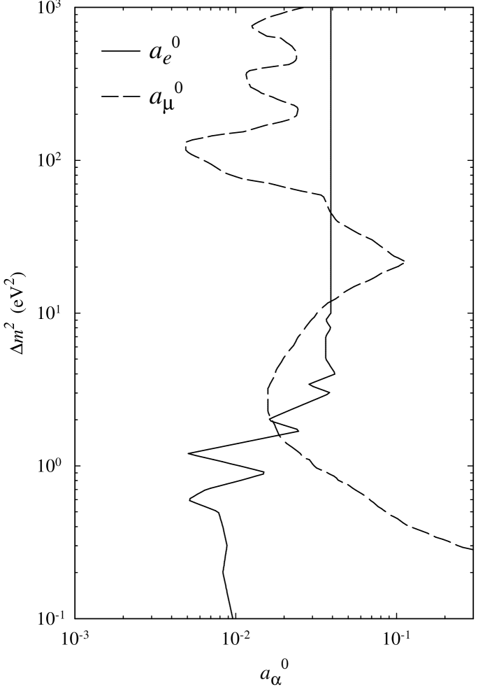
xxxxx

FIG. 2.: The bounds $a^{0}_{\alpha}$ ($\alpha=e,\mu$).

IV SBL disappearance experiments

For the two flavours $\alpha=e$ and $\mu$, results of disappearance experiments are available. We will use the 90% exclusion plots of the Bugey reactor experiment [34] for $\bar{\nu}_{e}$ disappearance and the 90% exclusion plots of the CDHS [35] and CCFR [36] accelerator experiments for $\nu_{\mu}$ disappearance. Since no neutrino disappearance has been seen in SBL experiments, there are upper bounds $B_{\alpha}^{0}$ on the disappearance amplitudes for $\alpha=e,\mu$. These experimental bounds are functions of $\Delta m^{2}_{\mbox{SBL}}$. It follows that

$$B_{\alpha}=4\,c_{\alpha}(1-c_{\alpha})\leq B_{\alpha}^{0}\quad\mbox{with}\quad c_{\alpha}\equiv\sum_{j=1}^{r}|U_{\alpha j}|^{2}$$ (18)

and, therefore [37],

$$c_{\alpha}\leq a^{0}_{\alpha}\quad\mbox{or}\quad c_{\alpha}\geq 1-a^{0}_{\alpha}\quad\mbox{with}\quad a^{0}_{\alpha}\equiv\frac{1}{2}\left(1-\sqrt{1-B_{\alpha}^{0}}\,\right)\,.$$ (19)

This equation formulates the important constraints on the mixing matrix $U$ stemming from the negative results of SBL disappearance neutrino oscillation experiments. Note that Eq.(19) shows that $a^{0}_{\alpha}\leq 1/2$. Furthermore, since the upper bounds $B_{\alpha}^{0}$ on the survival amplitudes $B_{\alpha}$ are functions of $\Delta m^{2}_{\mathrm{SBL}}$, the same is true for the bounds $a^{0}_{\alpha}$. In the region of $\Delta m^{2}_{\mathrm{SBL}}$ where no experimental restrictions on the survival amplitude are available, we have $B_{\alpha}^{0}\uparrow 1$, in which case it follows that $a^{0}_{\alpha}\uparrow 0.5$.

In Fig. 2 the bounds $a^{0}_{e}$ and $a^{0}_{\mu}$ are plotted as functions of $\Delta m^{2}_{\mathrm{SBL}}$ in the wide range $10^{-1}\;\mbox{eV}^{2}\leq\Delta m^{2}_{\mbox{SBL}}\leq 10^{3}\;\mbox{eV}^{2}$. In this range $a^{0}_{e}$ is small ($a^{0}_{e}\lesssim 4\times 10^{-2}$) and $a^{0}_{\mu}\lesssim 10^{-1}$ for $\Delta m^{2}_{\mbox{SBL}}\gtrsim 0.5$ eV².

V The LSND experiment

The LSND experiment investigates $\bar{\nu}_{\mu}\to\bar{\nu}_{e}$ oscillations, where the $\bar{\nu}_{\mu}$ flux is generated by $\mu^{+}$ decay at rest [14], and $\nu_{\mu}\to\nu_{e}$ oscillations, where the neutrino source is given by $\pi^{+}$ decay in flight [15]. Both channels have shown evidence in favour of neutrino oscillations with perfectly compatible results and, therefore, give a non-zero measurement of the transition amplitude $A_{\mu;e}$ (12). On the other hand, from the negative result of the Bugey experiment and from inequality (16) we also have the constraint

$$A_{\mu;e}\leq B^{0}_{e}\,.$$ (20)

From the 90% CL plot [16] of the LSND collaboration and from the Bugey bound $B^{0}_{e}$ one obtains approximately

$$2\times 10^{-3}\lesssim A_{\mu;e}\lesssim 4\times 10^{-2}$$ (21)

and

$$0.2\>\mbox{eV}^{2}\lesssim\Delta m^{2}_{\mathrm{SBL}}\lesssim 2\>\mbox{eV}^{2}\,.$$ (22)

See, e.g., also Fig. 5.9 in Ref. [24]. These ranges are also compatible with the negative result of the KARMEN experiment [38].

VI The Super-Kamiokande up-down asymmetry

In the Super-Kamiokande experiment – like before in the Kamiokande experiment – atmospheric electron and muon neutrinos are measured by the Cherenkov light of electrons and muons, respectively, produced by charged current interactions of the neutrinos. Thus, $e$-like events appear as diffuse rings and $\mu$-like events as sharp rings in the detector. A distinguished class of events is given by the single-ring (1r) events which are fully contained (FC) in the inner detector. These events are charged current $e$-like and $\mu$-like events with very high probability [9]. Partially contained (PC) events have tracks exiting the inner detector and are nearly 100% $\mu$-like events. The zenith angle distributions of Kamiokande [6] and Super-Kamiokande [9], which gave the first evidence for atmospheric neutrino oscillations, are based on such events, and the up-down asymmetry of Super-Kamiokande as well [9].

Note that in the Super-Kamiokande experiment muons going through [10] or stopping [11] in the detector are also measured, which originate from atmospheric muon neutrinos interacting with the rock beneath the detector. Evaluating these events under the hypothesis of neutrino oscillations gives results for $\Delta m^{2}_{\mathrm{atm}}$ and the atmospheric mixing angle compatible with the oscillation parameters derived from the zenith angle distribution [10, 11, 12]. The same applies to the result of the MACRO experiment on through-going muon events [13]. Moreover, these types of events, which correspond to neutrino energies of $E\sim 100$ GeV for the through-going and $E\sim 10$ GeV for the stopping events, have the capacity to allow for a distinction between the $\nu_{\mu}\to\nu_{\tau}$ and $\nu_{\mu}\to\nu_{s}$ solutions of the atmospheric neutrino anomaly. At present, the sterile neutrino solution is disfavoured at about 95% CL [39].

The zenith angle $\theta_{z}$ of an $e$-like or $\mu$-like event is defined as the angle between the vertical line and the direction of the electron or muon track. For multi-GeV events, defined by a visible energy larger than 1.33 GeV, the average angle between the charged lepton direction and the neutrino direction is around $20^{\circ}$ [9]. Since $\cos\theta_{z}=\pm 0.2$ corresponds to $90^{\circ}\pm 11.5^{\circ}$ it is reasonable to define up (U) and down (D) going $\mu$-like events in the following way:

$$\begin{array}[]{rl}U=\#(\mbox{multi GeV FC 1r + PC $\mu$-like events with}&-1\leq\cos\theta_{z}\leq-0.2)\,,\\ D=\#(\mbox{multi GeV FC 1r + PC $\mu$-like events with}&\hphantom{-}1\geq\cos\theta_{z}\geq\hphantom{-}0.2)\,.\end{array}$$ (23)

Clearly, if there are no neutrino oscillations, we would have $U=D$. Super-Kamiokande has measured the up-down asymmetry with the latest result [12]

$$A_{\mu}=\frac{U-D}{U+D}=-0.311\pm 0.043\pm 0.01\,.$$ (24)

This value constitutes the most compelling evidence for neutrino oscillations at present. The error $\pm 0.01$ stems from an estimation of the up-down asymmetric effects of the magnetic field of the earth on the primary cosmic ray flux. The value for the corresponding asymmetry for $e$-like events (defined via (23) but without PC) is given by $A_{e}=-0.036\pm 0.067\pm 0.02$ [9] and is compatible with zero, i.e., no oscillations of atmospheric electron neutrinos.

VII The 4-neutrino mass hierarchy is disfavoured by the data

In the case of a neutrino mass hierarchy, $m_{1}\ll m_{2}\ll m_{3}\ll m_{4}$, the mass-squared differences $\Delta{m}^{2}_{21}$ and $\Delta{m}^{2}_{32}\simeq\Delta{m}^{2}_{31}$ are relevant for the suppression of the flux of solar neutrinos and for the atmospheric neutrino anomaly, respectively. In this case the quantity $c_{\alpha}$ is defined via $r=3$ (see the formalism in Section III A and the definition (18)) and, therefore, we have

$$c_{\alpha}=\sum_{j=1}^{3}|U_{\alpha j}|^{2}\,.$$ (25)

In the following, according to the 4-neutrino assumption, we assume that $\Delta m^{2}_{\mathrm{SBL}}$ is in the numerical range (22) given by the result of the LSND experiment. Our aim is to derive three bounds on $c_{\mu}$ as functions of $\Delta m^{2}_{\mathrm{SBL}}$, using as input various oscillation data. We will finally see that these bound are incompatible with each other, thus strongly disfavouring the hierarchical neutrino mass spectrum.

The first bound we need is given by Eq.(19):

$$\mbox{Bound a:}\quad c_{\mu}\leq a^{0}_{\mu}\quad\mbox{or}\quad c_{\mu}\geq 1-a^{0}_{\mu}\,.$$ (26)

For this bound the experimental input is the data on SBL $\stackrel{{\scriptstyle\scriptscriptstyle(-)}}{{\nu}}_{\hskip-3.0pt\mu}$ disappearance [35, 36].

For the derivation of the next bound we refer the reader to Ref. [32]. It is based on the up-down asymmetry [9, 12]:

$$\mbox{Bound b:}\quad-A_{\mu}\leq\frac{c_{\mu}^{2}+2\,a^{0}_{e}(1-a^{0}_{e})/r}{c_{\mu}^{2}+2(1-c_{\mu})^{2}}\,,$$ (27)

where $r\equiv n_{\mu}/n_{e}$ is defined as the ratio of $\mu$-like to $e$-like events in the detector without neutrino oscillations. Its numerical value $r\simeq 2.8$ can be read off from Fig. 3 in Ref. [9]. Because of the smallness of $a^{0}_{e}$ the bound (27) has a very weak dependence on the precise value of $r$. For the bound (27), in addition to $A_{\mu}$, also SBL disappearance data [34] have been used and the lower bound on the survival probability of solar neutrinos given by [40] $P^{\odot}_{\nu_{e}\to\nu_{e}}\geq|U_{e4}|^{4}=(1-c_{e})^{2}$. The latter inequality shows that only the possibility $c_{e}\geq 1-a^{0}_{e}$ is allowed.

The third bound uses the fact that the LSND result establishes a lower bound $A_{\mu;e}^{\mathrm{min}}$ on the transition amplitude $A_{\mu;e}$:

$$\mbox{Bound c:}\quad c_{\mu}\leq 1-A^{\mathrm{min}}_{\mu;e}/4a^{0}_{e}\,.$$ (28)

It derives from $A_{\mu;e}=4(1-c_{e})(1-c_{\mu})$ (see Eq.(12)) and $c_{e}\geq 1-a^{0}_{e}$.

In Fig. 3 the bounds a, b, c, labelled by CDHS, SK+Bugey, LSND+Bugey, respectively, are plotted in the $\Delta{m}^{2}_{\mathrm{SBL}}$–$c_{\mu}$ plane. Note that bound c is practically a horizontal line due to the smallness of the term containing $a^{0}_{e}$. The three bounds, which are all derived from 90% CL data, leave no allowed region in the plot. Thus the hierarchical mass spectrum (I) is strongly disfavoured by the data. The same arguments presented here can be used also for the other spectra (II), (III), (IV) of class 1 (see Fig. 1) by defining $c_{\alpha}$ (18) through a summation over the indices of the three close masses for each of the spectra of class 1 [32].

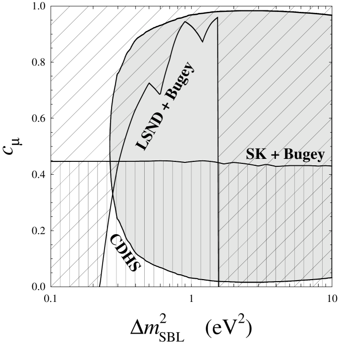
FIG. 3.: Regions in the $\Delta{m}^{2}_{\mathrm{SBL}}$–$c_{\mu}$ plane disfavoured by the results of the CDHS, CCFR, LSND, Super-Kamiokande and Bugey experiments in the case of the spectra of class 1. The shaded region is excluded by the inequalities (26) and the region with oblique hatching by the bound (28). The nearly horizontal curve labelled SK + Bugey represents the lower bound (27) derived from the Super-Kamiokande up–down asymmetry. No allowed region is left in this plot and, therefore, the spectra of class 1 are disfavoured by the data.

VIII The favoured 4-neutrino mass spectra (A) and (B)

Now we are left with only two possible neutrino mass spectra in which the four neutrino masses appear in two pairs separated by $\sim 1\,\mathrm{eV}$ [29, 30]:

$$\mbox{(A)}\quad\underbrace{\overbrace{m_{1}<m_{2}}^{\mbox{atm}}\ll\overbrace{m_{3}<m_{4}}^{\mbox{solar}}}_{\mbox{LSND}}\qquad\mbox{and}\qquad\mbox{(B)}\quad\underbrace{\overbrace{m_{1}<m_{2}}^{\mbox{solar}}\ll\overbrace{m_{3}<m_{4}}^{\mbox{atm}}}_{\mbox{LSND}}\;.$$ (29)

In the case of these two mass spectra we have $r=2$ and thus

$$c_{\alpha}=\sum_{j=1,2}|U_{\alpha j}|^{2}\quad(\alpha=e,\mu)\,.$$ (30)

With the argument analogous to the one using $P^{\odot}_{\nu_{e}\to\nu_{e}}$ below Eq.(27) one finds the following constraint on the mixing matrix:

$$\mbox{(A)}\quad c_{e}\leq a^{0}_{e}\,,\quad\mbox{(B)}\quad c_{e}\geq 1-a^{0}_{e}\,.$$ (31)

 

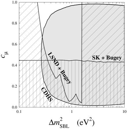
(a) Scheme (A)

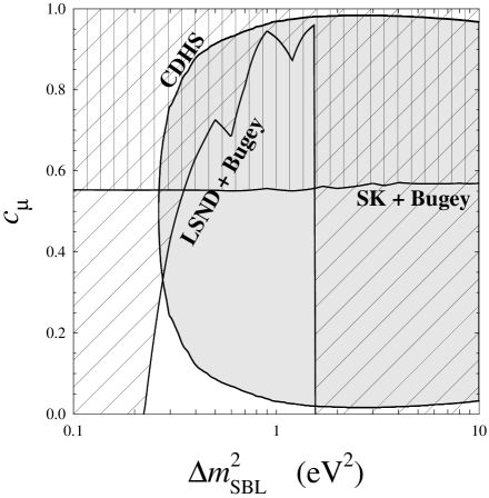
(b) Scheme (B)

FIG. 4.: The bounds for Schemes (A) and (B) analogous to the ones depicted in Fig. 3 in the case of the hierarchical mass spectrum. The white areas in Subfigs. (a) and (b) show the allowed regions of $c_{\mu}$ for Schemes (A) and (B), respectively. Subfig. (b) is obtained by reflection of all the curves in Subfig. (a) at the line $c_{\mu}=1/2$.

We have to check that these mass spectra are compatible with the results of all neutrino oscillation experiments. Going through the same arguments as in the case of the hierarchical mass scheme in the previous section, we have plotted the corresponding bounds a, b, c in Fig. 4 for Scheme (A) (Subfig. (a)) and (B) (Subfig. (b)). We observe that in these cases white areas (unshaded and unhatched) are left [32] which show the allowed ranges of $c_{\mu}$ in the $\Delta{m}^{2}_{\mathrm{SBL}}$–$c_{\mu}$ plane. Thus, Schemes (A) and (B) are compatible with all oscillation data.

IX The sterile neutrino and big-bang nucleosynthesis

Since we are discussing four neutrinos it is necessary to study the compatibility of the preferred Schemes (A) and (B) with BBN. Whether the effective number $N_{\nu}$ of light neutrinos relevant in BBN is smaller than 4, is still debated in the literature. An upper bound on $N_{\nu}$ depends, in particular, on the primordial deuterium abundance $(D/H)_{P}$ for which conflicting measurements exist. For the low value of $(D/H)_{P}$ the value of $N_{\nu}$ should rather be close to 3 [41] whereas a high ratio $(D/H)_{P}$ allows also values of $N_{\nu}$ around 4 [42]. In this section we inquire constraints on the mixing matrix $U$ under the assumption of $N_{\nu}<4$. In this case, a large active – sterile neutrino mixing seems to be excluded by standard BBN with zero lepton number asymmetry (see Refs. [43, 30, 44] and citations therein).

In a simplified version, the amount of sterile neutrinos present at BBN can be calculated using the differential equation [45]

$$\frac{dn_{\nu_{s}}}{dt}=\frac{1}{2}\sum_{\alpha=e,\mu,\tau}\langle P_{\nu_{\alpha}\to\nu_{s}}\rangle_{\mathrm{coll}}\Gamma_{\nu_{\alpha}}(1-n_{\nu_{s}})\,,$$ (32)

where $n_{\nu_{s}}$ is the number density of the sterile neutrino relative to the number density of an active neutrino in thermal equilibrium ($n_{\nu_{s}}\leq 1$) and the $\Gamma_{\nu_{\alpha}}$ are the total collision rates of the active neutrinos [46]. The oscillation probabilities in Eq.(32) are averaged over the collision time $t_{\mathrm{coll}}=1/\Gamma_{\nu_{e}}$. Eq.(32) is valid if the oscillation time is smaller than the collision time and if in the time evolution no resonance is encountered or a resonance is undergone adiabatically. For a further discussion of (32) see Ref. [44].

It turns out that in the time evolution in the early universe from a temperature of around 100 MeV to a few MeV, when the active neutrinos decouple, in Scheme (A) there is no resonance, whereas in Scheme (B) the time evolution goes through a non-adiabatic resonance. In the latter case the Landau–Zener effect has to be used to estimate the amount of sterile neutrinos produced at the resonance, instead of using Eq.(32). In this way the following constraint on $U$ can be derived [44]:

$$N_{\nu}<3.9\;\Rightarrow\;\left\{\begin{array}[]{rclc}c_{s}&<5\times 10^{-3}&\mbox{(A)}\,,\\ 1-c_{s}&<5\times 10^{-5}&\mbox{(B)}\,,\end{array}\right.$$ (33)

where $c_{s}=\sum_{j=1,2}|U_{sj}|^{2}$.

Thus, concentrating on Scheme (A), from Eqs.(31) and (33) and from Fig. 4 we know which elements in the mixing matrix must be small in the rows pertaining to the neutrino flavours (types) $e$, $\mu$ and $s$. Consequently, also the small elements in the $\tau$ row of $U$ are fixed. Symbolizing by $\circ$ small mixing elements and by $\bullet$ large ones, we arrive at the following mixing matrix:

$$\begin{array}[]{ccc}&\begin{array}[]{cccc}1&2&3&4\end{array}&\\ \mbox{Scheme (A):}\quad U=\!\!&\left(\begin{array}[]{cccc}\circ&\circ&\bullet&\bullet\\ \bullet&\bullet&\circ&\circ\\ \bullet&\bullet&\circ&\circ\\ \circ&\circ&\bullet&\bullet\end{array}\right)&\!\!\!\begin{array}[]{c}e\\ \mu\\ \tau\\ s\end{array}\end{array}$$ (34)

For Scheme (B) the analogous mixing matrix is obtained by the exchange $1\leftrightarrow 3$, $2\leftrightarrow 4$ of the columns in (34). As a consequence, if $N_{\nu}<4$, the solar neutrino problem is solved $\nu_{e}\to\nu_{s}$ transitions in Schemes (A) and (B), whereas the atmospheric neutrino anomaly by $\nu_{\mu}\to\nu_{\tau}$ transitions [30, 44]. Since a large mixing angle $\nu_{e}\to\nu_{s}$ transition as a solution of the solar neutrino puzzle is not compatible with the solar neutrino data [47], this transition must take place due to the small mixing angle MSW effect.

There is a debate in the literature if the constraint (33) can be avoided by taking into account the effect of a lepton number asymmetry in the early universe. It rather seems that this is not possible with the range (22) of $\Delta m^{2}_{\mathrm{SBL}}$ determined by the LSND experiment. For recent papers on this problem see Refs. [43, 48].

X Predictions of the favoured Schemes (A) and (B)

Schemes (A) and (B), either with or without the constraints from BBN, allow to make predictions for LBL and SBL experiments, CP violation in LBL experiments, ³H decay and $(\beta\beta)_{0\nu}$ decay. We will not touch the subject of CP violation (see the papers in Ref. [49]).

LBL experiments:
LBL neutrino oscillation experiments are sensitive to the so-called “atmospheric $\Delta m^{2}$ range” of $10^{-2}$–$10^{-3}$ eV². For reactor experiments with $E\sim 1$ MeV this requires $L\sim 1$ km [50], whereas in accelerator experiments with $E\sim 1$–10 GeV the length $L$ of the baseline is of order of a few 100 to 1000 km [51, 52, 53] (see Eq.(3)).

Let us consider scheme (A) and neutrinos for definiteness. Then in vacuum the probabilities of $\nu_{\alpha}\to\nu_{\beta}$ transitions in LBL experiments are given by

$$P^{(\mathrm{LBL,A})}_{\nu_{\alpha}\to\nu_{\beta}}=\left|U_{\beta 1}\,U_{\alpha 1}^{*}+U_{\beta 2}\,U_{\alpha 2}^{*}\,\exp\left(-i\frac{\Delta m^{2}_{\mathrm{atm}}L}{2E}\right)\right|^{2}+\Bigg{|}\sum_{k=3,4}U_{{\beta}k}\,U_{{\alpha}k}^{*}\Bigg{|}^{2}\,.$$ (35)

This formula has been obtained from Eq.(2) by dropping terms with large phases being approximately $\Delta m^{2}_{\mathrm{SBL}}L/2E$, which do not contribute to the oscillation probabilities averaged over the neutrino energy spectrum.

From Eq.(35), with $\alpha=\beta$ and Eq.(30), it follows immediately that

$$P^{(\mathrm{LBL,A})}_{\nu_{\alpha}\to\nu_{\alpha}}\geq(1-c_{\alpha})^{2}\,.$$ (36)

Applying this inequality to LBL reactor experiments we obtain [54]

$$1-P^{(\mathrm{LBL})}_{\bar{\nu}_{e}\to\bar{\nu}_{e}}\leq a^{0}_{e}\,(2-a^{0}_{e})\,.$$ (37)

One can easily check that Eq.(37) holds for both Schemes (A) and (B). In Fig. 5 we have plotted this bound together with the present experimental bound achieved in the CHOOZ experiment [50]. The negative result of the CHOOZ experiment is in agreement with the predictions of Schemes (A) and (B).

Considering now LBL transition probabilities and using the Cauchy–Schwarz inequality for the first term on the right-hand side of Eq.(35), we obtain

$$P^{(\mathrm{LBL,A})}_{\nu_{\alpha}\to\nu_{\beta}}\leq c_{\alpha}\,c_{\beta}+\frac{1}{4}\,A_{\alpha;\beta}\quad(\alpha\neq\beta)\,.$$ (38)

Whereas for the inequality (37) matter corrections play no role due to the small energy of reactor neutrinos and the distance $L\sim 1$ km of the detector from the source, such corrections have to be taken into account to derive a realistic bound from Eq.(38) in order to apply it to LBL accelerator experiments [51, 52, 53]. For a derivation of a matter-corrected, scheme-independent upper bound from Eq.(38) see Ref. [54]. For the MINOS and ICARUS experiments this upper bound on the $\nu_{\mu}\to\nu_{e}$ transition probability decreases from around 0.1 to 0.03 when $\Delta m^{2}_{\mathrm{SBL}}$ varies from 0.2 to 2 eV² (22) [54]. However, the sensitivity of these experiments is much better than this bound. For the KEK to Super-Kamiokande LBL experiment the upper bound on the same transition is rather 0.04 at most [54]. A similar stringent bound can be derived on the probability of $\nu_{e}\to\nu_{\tau}$ transitions.

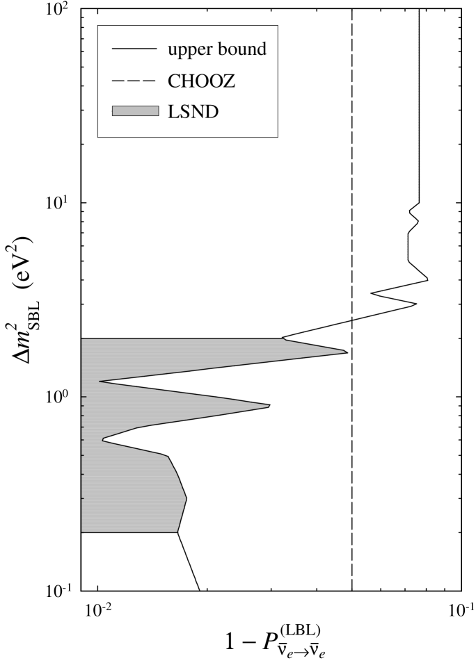
FIG. 5.: The upper bound (37) on $1-P^{(\mathrm{LBL})}_{\bar{\nu}_{e}\to\bar{\nu}_{e}}$. The shaded area indicates the LSND range (22) and the vertical dashed line the experimental upper bound which has been obtained in the CHOOZ experiment.

SBL $\nu_{\mu}\to\nu_{\tau}$ transitions:
If $N_{\nu}<4$ holds (see previous section), then the quantity $c_{s}$ is very small (see Eq.(33)). In this case it can be shown that

$$\left.\begin{array}[]{cr}\mbox{(A)}&c_{s}\to 0\\ \mbox{(B)}&1-c_{s}\to 0\end{array}\right\}\;\Rightarrow\;A_{\mu;\tau}\leq(a^{0}_{e})^{2}$$ (39)

is valid [44]. Due to the smallness of $a^{0}_{e}$ (see Fig. 2) the transition amplitude $A_{\mu;\tau}$ is below $10^{-3}$ [44], which also serves as a check for the validity of the BBN constraint on $U$.

³H decay:
Let us assume that $m_{1,2}\ll m_{3,4}$. Then one easily derives the relations [29]

$$\begin{array}[]{cl}\mbox{(A)}&m_{\nu}(^{3}\mbox{H})\simeq m_{3}\simeq m_{4}\,,\\ \mbox{(B)}&m_{\nu}(^{3}\mbox{H})\lesssim a^{0}_{e}m_{4}\end{array}$$ (40)

for the mass $m_{\nu}(^{3}\mbox{H})$ measured in tritium decay. Since in Scheme (A) one has $m_{3,4}\simeq(\Delta m^{2}_{\mathrm{SBL}})^{1/2}$, it might be possible in the future to see a neutrino mass in tritium decay, whereas this mass effect is suppressed in Scheme (B).

$(\beta\beta)_{0\nu}$ decay:
If neutrinos are of Majorana nature, neutrinoless double-beta decay proceeds via the effective Majorana neutrino mass (see Ref. [55] for other mechanisms)

$$|\langle m\rangle|=\left|\sum_{j=1}^{4}U^{2}_{ej}m_{j}\right|\,,$$ (41)

which can thus be related to present experimental information. Making the same assumptions about the neutrino masses as in the previous paragraph, it is easy to show that in Scheme (A) the relation

$$\sqrt{1-\sin^{2}2\theta_{\mathrm{solar}}}\sqrt{\Delta m^{2}_{\mathrm{SBL}}}\lesssim|\langle m\rangle|\lesssim\sqrt{\Delta m^{2}_{\mathrm{SBL}}}$$ (42)

holds [56], where $\theta_{\mathrm{solar}}$ is the mixing angle relevant for solar neutrino oscillations. Note that from the range (22) it follows that

$$0.5\;\mbox{eV}\lesssim\sqrt{\Delta m^{2}_{\mathrm{SBL}}}\lesssim 1.4\;\mbox{eV}.$$ (43)

Thus, at least the upper bound in Eq.(42) is in the reach of present experiments [57, 58]. At present a very stringent bound exists from the ⁷⁶Ge experiment [58] with $|\langle m\rangle|\lesssim 0.2\div 0.6$ eV (see also the references cited in Ref. [58]). Note that for the small mixing angle MSW solution of the solar neutrino puzzle, which is favoured by BBN, one has

$$|\langle m\rangle|\simeq\sqrt{\Delta m^{2}_{\mathrm{SBL}}}\,.$$ (44)

XI Conclusions

In this report we have discussed the possible form of the neutrino mass spectrum that can be inferred from the results of all neutrino oscillation experiments, including solar and atmospheric neutrino experiments. The crucial input are the three indications in favour of neutrino oscillations given by the solar neutrino data, the atmospheric neutrino anomaly and the result of the LSND experiment, and also the negative results of the SBL disappearance experiments. These indications, which all pertain to different scales of neutrino mass-squared differences, require that apart from the three well-know neutrino flavours at least one additional sterile neutrino (without couplings to the $W$ and $Z$ bosons) must exist. In our investigation we have assumed that there is one sterile neutrino and that the 4-neutrino mixing matrix (1) is unitary. We have considered all possible schemes with four massive neutrinos which provide three scales of $\Delta{m}^{2}$ (see Fig. 1).

The main points of our discussion can be summarized as follows:

• The data prefer the non-hierarchical mass spectra (A) and (B) (see Fig. 1 and Eq.(29)) with two pairs of close masses separated by a mass difference of the order of 1 eV necessary for a description of the LSND result. In Scheme (A), the quantity $|U_{e1}|^{2}+|U_{e2}|^{2}$ is small and $|U_{\mu 1}|^{2}+|U_{\mu 2}|^{2}$ is close to 1, and vice versa in Scheme (B).

• The solar neutrino problem is preferably solved by $\nu_{e}\to\nu_{\tau},\nu_{s}$ and the atmospheric neutrino anomaly by $\nu_{\mu}\to\nu_{\tau},\nu_{s}$ transitions. If the effective number $N_{\nu}$ of neutrinos relevant in BBN is smaller than 4, then standard BBN leads to small mixing angle MSW $\nu_{e}\to\nu_{s}$ transitions as the solution of the solar neutrino problem and to $\nu_{\mu}\to\nu_{\tau}$ transitions in atmospheric neutrinos.

• Again with $N_{\nu}<4$, $\nu_{\mu}\to\nu_{\tau}$ transitions are strongly suppressed in SBL neutrino oscillations. Note that in the case of $N_{\nu}<4$ all SBL neutrino oscillations are small or suppressed.

• In LBL neutrino oscillations, it follows from Schemes (A) and (B) that the transitions $\nu_{e}\to\nu_{\alpha}\;(\alpha\neq e)$ and $\nu_{\mu}\to\nu_{e}$ are suppressed.

• Schemes (A) and (B) could in principle be distinguished in ³H and $(\beta\beta)_{0\nu}$ decays, because in Scheme (A) neutrino mass effects are expected, whereas in Scheme (B) such effects are suppressed. Note that in Scheme (A) with the small mixing angle MSW solution of the solar neutrino problem, which is preferred by standard BBN (see Section IX), one gets $|\langle m\rangle|\simeq\sqrt{\Delta m^{2}_{\mathrm{SBL}}}\gtrsim 0.5$ eV for the effective Majorana mass relevant in $(\beta\beta)_{0\nu}$ decay (see Eqs.(42) and (43)). Such a large value for $|\langle m\rangle|$ should be close to discovery.

Finally, we want to remark that the most crucial input in our discussion is the result of the LSND experiment. This result will be checked by the approved MiniBooNE experiment, which will begin data taking in 2001 [59, 60]. The SNO experiment, which is expected to announce the first results in 2000, will test the hypothesis of oscillations of solar neutrinos into sterile neutrinos [61]. It could thus deliver a very important further piece of evidence in favour of the sterile neutrino and thus indirectly also check the BBN constraint on the 4-neutrino mixing matrix.

REFERENCES

- [1] B.T. Cleveland et al., Astrophys. J. 496, 505 (1998).
- [2] Kamiokande Coll., K.S. Hirata et al., Phys. Rev. D 44, 2241 (1991).
- [3] GALLEX Coll., W. Hampel et al., Phys. Lett. B 388, 384 (1996).
- [4] SAGE Coll., J.N. Abdurashitov et al., Phys. Rev. Lett. 77, 4708 (1996).
- [5] Super-Kamiokande Coll., M.B. Smy, talk presented at the DPF’99 Conference, hep-ph/9903034; Super-Kamiokande Coll., Y. Fukuda et al., Phys. Rev. Lett 82, 2430 (1999); Super-Kamiokande Coll., Y. Fukuda, T. Hayakawa, E. Ichihara and K. Inoue, Phys. Rev. Lett 82, 1810 (1999).
- [6] Kamiokande Coll., Y. Fukuda et al., Phys. Lett. B 335, 237 (1994).
- [7] IMB Coll., R. Becker-Szendy et al., Nucl. Phys. B (Proc. Suppl.) 38, 331 (1995).
- [8] Soudan Coll., W.W.M. Allison et al., Phys. Lett. B 391, 491 (1997).
- [9] Super-Kamiokande Coll., Y. Fukuda et al., Phys. Rev. Lett. 81, 1562 (1998).
- [10] Super-Kamiokande Coll., Y. Fukuda et al., Phys. Rev. Lett. 82, 2644 (1999).
- [11] Super-Kamiokande Coll., Y. Fukuda et al., hep-ex/9908049.
- [12] Super-Kamiokande Coll., K. Scholberg, Talk presented at 8th International Workshop on Neutrino Telescopes, Venice, February 23–26, 1999, hep-ex/9905016.
- [13] MACRO Coll., M. Ambrosio et al., Phys. Lett. B 434, 451 (1998).
- [14] LSND Coll., C. Athanassopoulos et al., Phys. Rev. Lett. 77, 3082 (1996).
- [15] LSND Coll., C. Athanassopoulos et al., Phys. Rev. Lett. 81, 1774 (1998).
- [16] LSND WWW page: http://www.neutrino.lanl.gov/neutrino/.
- [17] Particle Data Group, C. Caso et al., Eur. Phys. J. C 3, 1.
- [18] R.N. Mohapatra and P.B. Pal, “Massive Neutrinos in Physics and Astrophysics”, World Scientific Lecture Notes in Physics, Vol. 41, World Scientific, Singapore, 1991.
- [19] Z. Maki, M. Nakagawa and S. Sakata, Prog. Theor. Phys. 28, 870 (1962).
-
[20]
R.N. Mohapatra,
Talk presented at the COSMO98 Workshop,
hep-ph/9903261. - [21] B. Pontecorvo, Sov. Phys. JETP 26, 984 (1968); S.M. Bilenky and B. Pontecorvo, Phys. Rep. 41, 225 (1978); S.M. Bilenky and S.T. Petcov, Rev. Mod. Phys. 59, 671 (1987).
- [22] S.M. Bilenky, hep-ph/9908335.
- [23] C.W. Kim and A. Pevsner, “Neutrinos in Physics and Astrophysics”, Contemporary Concepts in Physics, Vol. 8, Harwood Academic Press, Chur, Switzerland, 1993; M. Zrałek, Acta Phys. Polon. B 29, 3925 (1998); W. Grimus, S. Mohanty and P. Stockinger, hep-ph/9909341.
- [24] S.M. Bilenky, C. Giunti and W. Grimus, hep-ph/9812360, to appear in Prog. Part. Nucl. Phys. 43.
- [25] J.N. Bahcall, P.I. Krastev and A.Yu. Smirnov, Phys. Rev. D 58, 096016 (1998).
- [26] M.C. Gonzalez-Garcia et al., hep-ph/9906469.
- [27] S.P. Mikheyev and A.Yu. Smirnov, Yad. Fiz. 42, 1441 (1985) [Sov. J. Nucl. Phys. 42, 913 (1985)]; Il Nuovo Cimento C 9, 17 (1986); L. Wolfenstein, Phys. Rev. D 17, 2369 (1978); ibid. 20, 2634 (1979).
- [28] J.T. Peltoniemi, D. Tommasini and J.W.F. Valle, Phys. Lett. B 298, 383 (1993); J.T. Peltoniemi and J.W.F. Valle, Nucl. Phys. B 406, 409 (1993); D.O. Caldwell and R.N. Mohapatra, Phys. Rev. D 48, 3259 (1993); E. Ma and P. Roy, ibid 52, R4780 (1995); E.J. Chun et al., Phys. Lett. B 357, 608 (1995); J.J. Gomez-Cadenas and M.C. Gonzalez-Garcia, Z. Phys. C 71, 443 (1996); E. Ma, Mod. Phys. Lett. A 11, 1893 (1996); S. Goswami, Phys. Rev. D 55, 2931 (1997).
- [29] S.M. Bilenky, C. Giunti and W. Grimus, Proc. of Neutrino ’96, Helsinki, June 1996, edited by K. Enqvist et al., p.174 (World Scientific, Singapore, 1997); Eur. Phys. J. C 1, 247 (1998).
- [30] N. Okada and O. Yasuda, Int. J. Mod. Phys. A 12, 3669 (1997).
- [31] V. Barger, S. Pakvasa, T.J. Weiler and K. Whisnant, Phys. Rev. D 58, 093016 (1998).
- [32] S.M. Bilenky, C. Giunti, W. Grimus and T. Schwetz, Phys. Rev. D 60, 073007 (1999).
- [33] S.M. Bilenky, C. Giunti and W. Grimus, Contribution to WHEPP-5, Pune, India, January 12–26, 1998, Pramana 51, 51 (1998).
- [34] B. Achkar et al., Nucl. Phys. B 434, 503 (1995).
- [35] F. Dydak et al., Phys. Lett. B 134, 281 (1984).
- [36] I.E. Stockdale et al., Phys. Rev. Lett. 52, 1384 (1984).
- [37] S.M. Bilenky, A. Bottino, C. Giunti and C.W. Kim, Phys. Lett. B 356, 273 (1995); Phys. Rev. D 54, 1881 (1996).
- [38] KARMEN Coll., K. Eitel et al., Contribution to 18th International Conference on Neutrino Physics and Astrophysics (NEUTRINO 98), Takayama, Japan, June 4–9, 1998, Nucl. Phys. (Proc. Suppl.) 77, 212 (1999).
- [39] Super-Kamiokande Coll., M. Nakahata, Talk presented at TAUP ’99, WWW page: http://taup99.in2p3.fr/TAUP99/.
- [40] S.M. Bilenky, C. Giunti, C.W. Kim and S.T. Petcov, Phys. Rev. D 54, 4432 (1996).
- [41] S. Burles et al., Phys. Rev. Lett. 82, 4176 (1999).
- [42] K.A. Olive and D. Thomas, Astropart. Phys. 11, 403 (1999); E. Lisi, S. Sarkar and F.L. Villante, Phys. Rev. D 59, 123520 (1999); K.A. Olive, Talk delivered at the 19th Texas Symposium on Relativistic Astrophysics and Cosmology, Paris, France, December 1998, astro-ph/9903309.
- [43] X. Shi and G.M. Fuller, astro-ph/9904041.
- [44] S.M. Bilenky, C. Giunti, W. Grimus and T. Schwetz, Astropart. Phys. 11, 413 (1999).
- [45] K. Kainulainen, Phys. Lett. B 224, 191 (1990).
- [46] K. Enqvist, K. Kainulainen and M. Thomson, Nucl. Phys. B 373, 498 (1992).
- [47] P.I. Krastev and S.T. Petcov, Phys. Rev. D 53, 1665 (1996); P.I. Krastev, Q.Y. Liu and S.T. Petcov, Phys. Rev. D 54, 7057 (1996).
- [48] R. Foot and R.R. Volkas, astro-ph/9811067; X. Shi and G.M. Fuller, astro-ph/9812232; K. Abazajian, X. Shi and G.M. Fuller, astro-ph/9904052; M.V. Chizhov and D.P. Kirilova, hep-ph/9908525.
- [49] S.M. Bilenky, C. Giunti and W. Grimus, Phys. Rev. D 58, 033001 (1998); V. Barger, Y.-B. Dai, K. Whisnant and B.-L. Young, Phys. Rev. D 59, 113010 (1999); K. Dick, M. Freund, M.Lindner and A. Romanino, hep-ph/9903308, to be published in Nucl. Phys. B; A. Donini, M.B. Gavela, P. Hernández and S. Rigolin, hep-ph/9909254; A. Kalliomäki, J. Maalampi and M. Tanimoto, hep-ph/9909301.
- [50] CHOOZ Coll., M. Apollonio et al., hep-ex/9907037.
- [51] Y. Suzuki, Proc. of Neutrino ’96, Helsinki, June 1996, edited by K. Enqvist et al., p.237 (World Scientific, Singapore, 1997).
- [52] S.G. Wojcicki, Proc. of Neutrino ’96, Helsinki, June 1996, edited by K. Enqvist et al., p.231 (World Scientific, Singapore, 1997).
- [53] A. Bueno, Contribution to 5th International Workshop on Tau Lepton Physics (TAU 98), Santander, Spain, September 14–17, 1998. Nucl. Phys. (Proc. Suppl.) 76, 463 (1999).
- [54] S.M. Bilenky, C. Giunti and W. Grimus, Phys. Rev. D 57 (1998) 1920.
- [55] R.N. Mohapatra, Talk presented at 18th International Conference on Neutrino Physics and Astrophysics (NEUTRINO 98), Takayama, Japan, June 4–9, 1998, Nucl. Phys. (Proc. Suppl.) 77, 376 (1999).
- [56] S.M. Bilenky, C. Giunti, W. Grimus, B. Kayser and S.T. Petcov, hep-ph/9907234, to be published in Phys. Lett. B.
- [57] A. Faessler and F. Šimkovic, J. Phys. G 24, 2139 (1998).
- [58] L. Baudis et al., Phys. Rev. Lett. 83, 41 (1999).
- [59] J.M. Conrad, Talk presented at International Conference on High Energy Physics (ICHEP), Vancouver, 1998, hep-ex/9811009.
-
[60]
Booster Neutrino Experiment WWW page:
http://www.neutrino.lanl.gov/BooNE/. -
[61]
Sudbury Neutrino Observatory WWW page:
http://www.sno.phy.queensu.ca/.