KIAS-P99094

hep-ph/9910325

DETERMINING SUSY PARAMETERS IN CHARGINO PAIR
PRODUCTION IN $e^{+}e^{-}$ COLLISIONS

In most supersymmetric theories, charginos $\tilde{\chi}^{\pm}_{1,2}$ belong to the class of the lightest supersymmetric particles and they are easy to observe at $e^{+}e^{-}$ colliders. By measuring the total cross sections and the left–right asymmetries with polarized beams as well as the angular correlations of the decay products of the charginos in $e^{+}e^{-}\rightarrow\tilde{\chi}^{-}_{i}\tilde{\chi}^{+}_{j}\,[i,j=1,2]$, the chargino masses and the gaugino–higgsino mixing angles can be determined very accurately. From these observables the relevant fundamental SUSY parameters can be derived: $M_{2}$, $|\mu|$, $\cos\Phi_{\mu}$, and $\tan\beta=v_{2}/v_{1}$. The solutions are unique.

1 Introduction

In most supersymmetric theories, charginos $\tilde{\chi}^{\pm}_{1,2}$, mixtures of charged gauginos and higgsinos, belong to the class of the lightest supersymmetric particles and they are easy to observe at $e^{+}e^{-}$ colliders. Once the charginos are discovered, the priority will be to measure the low-energy SUSY parameters independently of theoretical models and then check whether the correlations among parameters support a given theoretical framework, like SUSY-GUT relations. For this purpose, it is very important that the $e^{+}e^{-}$ c.m. energy can be optimized to cross only very few thresholds at a time, and also to have beam polarization. Making judicious choices of these features, the confusing mixing of many final states with the cascade decays can be avoided and analyses restricted to a specific subset of processes performed.

In this contribution, we discuss methods of extracting SUSY parameters from the chargino sector. We analyze attempts of “measuring” the fundamental parameters at a $e^{+}e^{-}$ linear collider (LC) by taking two steps $\!{}^{{\bf?},{\bf?}}$: (I) From the observed quantities such as cross sections, polarization asymmetries, and angular correlations we determine the phenomenological parameters: the chargino masses and mixings, and (II) from the phenomenological parameters we extract the Lagrangian parameters: $M_{1,2}$, $\mu$, $\tan\beta$, and $m_{\tilde{\nu}}$. Each step can suffer from both experimental problems and theoretical ambiguities. An alternative approach for the step II, based only on the masses of some of the charginos and neutralinos, has been provided by Kneur and Moultaka $\!{}^{{\bf?}}$, and the polarization and spin effects in the neutralino system has been studied by Moortgat-Pick et al. $\!{}^{{\bf?}}$. In contrast, many earlier analyses $\!{}^{{\bf?}}$ have elaborated on global fits.

2 Determining SUSY parameters in the chargino system

The spin–1/2 superpartners of the $W$ boson and charged Higgs boson, $\tilde{W}^{\pm}$ and $\tilde{H}^{\pm}$, mix to form chargino mass eigenstates $\tilde{\chi}^{\pm}_{1,2}$ through the chargino mass matrix in the $(\tilde{W}^{-},\tilde{H}^{-})$ basis

$${\cal M}_{C}=\left(\begin{array}[]{cc}M_{2}&\sqrt{2}m_{W}c_{\beta}\\ \sqrt{2}m_{W}s_{\beta}&\mu\end{array}\right)$$ (3)

which is given in terms of fundamental parameters: $M_{2}$, $\mu$, and $\tan\beta=v_{2}/v_{1}$; $s_{\beta}=\sin\beta$, $c_{\beta}=\cos\beta$. In CP–noninvariant theories, the gaugino mass $M_{2}$ and the higgsino mass parameter $\mu$ can be complex. However, by reparametrization of the fields, $M_{2}$ can be assumed real and positive without loss of generality so that the only non–trivial invariant phase is attributed to $\mu$: $\mu=|\mu|\,{\rm e}^{i\Phi_{\mu}}$ ($0\leq\Phi_{\mu}\leq 2\pi$).

The complex, asymmetric chargino mass matrix ${\cal M}_{C}$ is diagonalized with two different unitary matrices $U_{L}$ and $U_{R}$ acting on the left– and right–chiral $(\tilde{W}^{-},\tilde{H}^{-})$ states, respectively, which can be parametrized in terms of the left/right mixing angles $\phi_{L,R}$, the left/right CP–violating phases $\{\beta_{L},\beta_{R}\}$ and two additional phases $\{\gamma_{1},\gamma_{2}\}$. These phases are not independent but can be expressed in terms of the invariant angle $\Phi_{\mu}$, and all of them vanish in CP–invariant theories for $\Phi_{\mu}=0$ or $\pi$. The mass eigenvalues $m^{2}_{\tilde{\chi}^{\pm}_{1,2}}$ and the rotation angles $\phi_{L}$ and $\phi_{R}$ are uniquely determined by the fundamental SUSY parameters $\{\tan\beta,M_{2},|\mu|,\cos\Phi_{\mu}\}$.

Charginos are produced either in diagonal or in mixed pairs in $e^{+}e^{-}$ collisions. With the second chargino $\tilde{\chi}_{2}^{\pm}$ expected to be significantly heavier than the first one, $\tilde{\chi}_{1}^{\pm}$ may be, for some time, the only chargino state that can be studied experimentally in detail in the first phase of a LC. Keeping in mind this point, we study two cases - (i) only the lightest charginos can be pair produced without beam polarization in the CP invariant theories and (ii) any pairs of chargino states can be produced with sufficient energies and beam polarization in the CP noninvariant theories.

2.1 Diagonal pair production of light charginos in the CP invariant theories

The $\tilde{\chi}^{-}_{1}\tilde{\chi}^{+}_{1}$ production cross section in $e^{+}e^{-}$ collisions depends on $m_{\tilde{\chi}^{\pm}_{1}}$, $m_{\tilde{\nu}}$ and the mixing angles $\phi_{L,R}$ and it increases very sharply near threshold, allowing the precise determination of the chargino mass.

Each of the charginos decay directly to a pair of fermions and the (stable) lightest neutralino $\tilde{\chi}_{1}^{0}$ through the exchange of a $W$ boson or scalar partners of fermions. In that case, two invisible neutralinos in the final state of the process, $e^{+}e^{-}\to\tilde{\chi}_{1}^{+}\tilde{\chi}_{1}^{-}\to\tilde{\chi}_{1}^{0}\tilde{\chi}_{1}^{0}(f_{1}\bar{f}_{2})(\bar{f}_{3}f_{4})$, makes it impossible to measure directly the chargino production angle $\Theta$ in the laboratory frame. Integrating over this angle and also over the invariant masses of the fermionic systems $(f_{1}\bar{f}_{2})$ and $(\bar{f}_{3}f_{4})$, we can write the fully–correlated distribution $\Sigma(\theta^{*},\phi^{*},\bar{\theta}^{*},\bar{\phi}^{*})$ in terms of sixteen independent angular combinations of helicity production amplitudes:

$$\Sigma = \Sigma_{\rm unp}+\kappa(\cos\theta^{*}+\cos\bar{\theta}^{*}){\cal P}-\kappa^{2}\left[\cos\theta^{*}\cos\bar{\theta^{*}}{\cal Q}\right.$$ (4)

$$\left.+\sin\theta^{*}\sin\bar{\theta^{*}}\cos(\phi^{*}+\bar{\phi^{*}}){\cal Y}\right]+\dots\,,$$

in the CP–invariant theory, where the analysis power $\kappa$ contains all the complicated dependence on the chargino decay dynamics such as neutralino and sfermion masses and their couplings, and $\theta^{*}$ is the polar angle of the $f_{1}\bar{f}_{2}$ system in the $\tilde{\chi}^{-}_{1}$ rest frame with respect to the chargino’s flight direction in the lab frame, and $\phi^{*}$ the azimuthal angle with respect to the production plane; quantities with a bar refer to the $\tilde{\chi}^{+}_{1}$ decay.

A crucial observation $\!{}^{{\bf?}}$ is that all explicitly written terms in eq. (4) can be extracted and three $\kappa$-independent physical observables, $\Sigma_{\rm unp},{\cal P}^{2}/{\cal Q}$ and ${\cal P}^{2}/{\cal Y}$, constructed by kinematical projections with $\cos\theta^{*},\cos\bar{\theta^{*}}$ and $\sin\theta^{*}\sin\bar{\theta^{*}}\cos(\phi^{*}+\bar{\phi^{*}})$ fully determined by the measurable parameters $E,|\vec{p}|$ (the energy and momentum of each of the decay systems $f_{i}\bar{f_{j}}$ in the laboratory frame) and the chargino mass. As a result, the chargino properties can be determined without any strong dependence on the other sectors of the model. The measurements of the cross section and either of the ratios ${\cal P}^{2}/{\cal Q}$ or ${\cal P}^{2}/{\cal Y}$, interpreted as contour lines in the plane $\{\cos 2\phi_{L},\cos 2\phi_{R}\}$, intersect at some discrete points to enable us to determine $\cos 2\phi_{L}$ and $\cos 2\phi_{R}$. An example for the determination of $\cos 2\phi_{L,R}$ is shown in fig. 1 for $m_{\tilde{\chi}^{\pm}_{1}}=95$ GeV and the “measured” observables; $\sigma_{tot}=0.37\,{\rm pb}$, ${\cal P}^{2}/{\cal Q}=-0.24$ and ${\cal P}^{2}/{\cal Y}=-3.66$ whose contour lines meet at a single point $\{\cos 2\phi_{L}=-0.8,\,\cos 2\phi_{R}=-0.5\}$ with $m_{\tilde{\nu}}=250$ GeV .

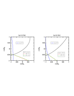
Figure 1: Contours for the “measured values” of the total cross section (solid line), ${\cal P}^{2}/{\cal Q}$, and ${\cal P}^{2}/{\cal Y}$ (dot-dashed line) for $m_{\tilde{\chi}_{1}^{\pm}}=95$ GeV [ $m_{\tilde{\nu}}=250$ GeV ]. For reference, the contour lines for the ”measured” LR asymmetry (solid, almost vertical lines) are also superimposed.

Let us now discuss the step II by describing briefly how to determine the SUSY $M_{2},\mu$ and $\tan\beta$ from $m_{\tilde{\chi}^{\pm}_{1}}$, $\cos 2\phi_{L}$ and $\cos 2\phi_{R}$ in the CP-invariant theory. It is most transparently achieved by introducing the two triangular quantities $p=\cot(\phi_{R}-\phi_{L})$ and $q=\cot(\phi_{R}+\phi_{L})$. They are expressed in terms of the measured values $x=\cos 2\phi_{L}$ and $y=\cos 2\phi_{R}$ up to a discrete ambiguity due to undetermined signs in $p^{2}-q^{2}$:

$$p^{2}+q^{2}=\frac{2(2-x^{2}-y^{2})}{(x-y)^{2}},\ \ pq=\frac{x+y}{x-y},\ \ p^{2}-q^{2}=\pm\frac{4\sqrt{(1-x^{2})(1-y^{2})}}{(x-y)^{2}}\,,$$ (5)

which enable us to find at most two possible solutions for $\tan\beta$, and then to determine $M_{2}/\mu=m_{W}[(p\pm q)s_{\beta}-(p\mp q)c_{\beta}]/\sqrt{2}$, respectively. The “measured values” given in the previous paragraph, for example, yield the results $\!{}^{{\bf?}}$; $[\tan\beta;M_{2},\mu]=[1.06;83\,{\rm GeV},-59\,{\rm GeV}]$ and $[3.33;248\,{\rm GeV},123\,{\rm GeV}]$.

To summarize, from the lightest chargino pair production, the measurements of the total production cross section and either the angular correlations among the chargino decay products (${\cal P}^{2}/{\cal Q}$, ${\cal P}^{2}/{\cal Y}$), $m_{\tilde{\chi}^{\pm}_{1}}$, $\cos 2\phi_{L}$ and $\cos 2\phi_{R}$ are determined unambiguously (Step I). Then the fundamental parameters $\tan\beta$, $M_{2}$ and $\mu$ are extracted up to a two-fold ambiguity (Step II). In addition, if polarized beams are available, the left–right (LR) asymmetry $A_{LR}$ can provide an alternative way to extract the mixing angles (or serve as a consistency check). This is also demonstrated in fig. 1, where contour lines for the “measured” values of $A_{LR}$ are shown.

2.2 Diagonal and non–diagonal pair production of charginos in the CP noninvariant theories

If the collider energy is sufficient to produce the two chargino states in pairs, the above ambiguity can be removed $\!{}^{{\bf?}}$. The new crucial ingredient in this case is the knowledge of the heavier chargino mass. Like for the lighter one, $m_{\tilde{\chi}^{\pm}_{2}}$ can be determined very precisely from the sharp rise of the production cross sections $\sigma(e^{+}e^{-}\rightarrow\tilde{\chi}^{-}_{i}\tilde{\chi}^{+}_{j})$. Moreover, the LR asymmetry $A_{LR}$ can provide a powerful way to extract the mixing angles without any detailed information on the chargino decay dynamics. We demonstrate this point based on the CP–invariant mSUGRA scenario RR1: $\{\tan\beta,m_{0},M_{\frac{1}{2}}\}=\{3,100\,{\rm GeV},200\,{\rm GeV}\}$, giving for the chargino/gaugino and sneutrino masses: $m_{\tilde{\chi}^{\pm}_{1,2}}=128/346\,{\rm GeV}$ and $m_{\tilde{\nu}}=166\,{\rm GeV}$. For the c.m. energy $\sqrt{s}=800$ GeV the scenario $RR1$ leads to the following values for the cross sections; $\sigma_{tot}(1,1)=0.197$ pb, $\sigma_{tot}(1,2)=0.068$ pb, and $\sigma_{tot}(2,2)=0.101$ pb, and the LR asymmetries; $A_{LR}(1.1)=-0.995$, $A_{LR}(1,2)=-0.911$, and $A_{LR}=-0.668$. Fig. 2 exhibits the contours in the plane $\{\cos 2\phi_{L},\cos 2\phi_{R}\}$ plane for the measured values of three cross sections and three LR asymmetries in the diagonal and mixed pair-production processes. All the contours meet at a common point: $[\cos 2\phi_{L},\cos 2\phi_{R}]=[0.67,0.85]$. Consequently, $\cos 2\phi_{L,R}$ along with the chargino masses are uniquely determined.

The measured phenomenological parameters - two chargino masses $m_{\tilde{\chi}^{\pm}_{1,2}}$ and the cosines of two mixing angles $\cos 2\phi_{L,R}$ - enable us to decode the basic SUSY parameters $\{\tan\beta,M_{2},|\mu|,\cos\Phi_{\mu}\}$: (i) $\tan\beta$ is uniquely determined in terms of two chargino masses and two mixing angles $\tan\beta=[4-\Delta_{\rm C}(x-y)]^{1/2}/[4+\Delta_{\rm C}(x-y)]^{1/2}$ with $\Delta_{\rm C}=(m^{2}_{\tilde{\chi}^{\pm}_{2}}-m^{2}_{\tilde{\chi}^{\pm}_{1}})/m^{2}_{W}$. (ii) based on the definition $M_{2}>0$, $M_{2}$ and $|\mu|$ reads $M_{2}/|\mu|=m_{W}[2\Sigma_{\rm C}\mp\Delta_{\rm C}(x+y)]^{1/2}/2$, respectively, with $\Sigma_{\rm C}=(m^{2}_{\tilde{\chi}^{\pm}_{2}}+m^{2}_{\tilde{\chi}^{\pm}_{1}}-2m^{2}_{W})/m^{2}_{W}$; (iii) $\cos\Phi_{\mu}$ is given by

$$\cos\Phi_{\mu}=\frac{\Delta^{2}_{\rm C}(2-x^{2}-y^{2})-8\Sigma_{\rm C}}{\sqrt{16-\Delta^{2}_{\rm C}(x-y)^{2}}\sqrt{4\Sigma^{2}_{\rm C}-\Delta^{2}_{\rm C}(x+y)^{2}}}\,.$$ (6)

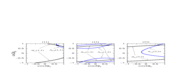
Figure 2: Contours in the $\{\cos 2\phi_{L},\cos 2\phi_{R}\}$ plane for ”measured values of $\sigma_{tot}(ij)$ and $A_{LR}(ij)$ $[i,j=1,2]$. The fat dot in each figure marks the common crossing point of the contours.

As a result, the fundamental SUSY parameters $\{\tan\beta,M_{2},|\mu|\,\cos\Phi_{\mu}\}$ in CP–noninvariant theories, can be extracted unambiguously from the observables $m_{\tilde{\chi}^{\pm}_{1,2}}$, $\cos 2\phi_{R}$, and $\cos 2\phi_{L}$. The final ambiguity in $\Phi_{\mu}\leftrightarrow 2\pi-\Phi_{\mu}$ may be resolved by measuring observables related to the normal polarization of charginos in non–diagonal chargino–pair production. In addition, it is worthwhile to note that the energy distribution of the final particles in the decay of the lightest chargino enables us to measure the mass of the lightest neutralino as well; this allows us to determine the other gaugino mass parameter $M_{1}$ if it is real. Otherwise, additional information on the phase of $M_{1}$ must be derived from observables involving the heavier neutralinos.

Table 1: Mean values and statistical uncertainties of $\{\tan\beta,M_{2},\mu\}$ obtained with the integrated luminosity of 500 fb^-1 in $RR1$ and $RR2$.

	$RR1$	$RR2$
$\tan\beta$	$3\pm 0.7$	—
$M_{2}$ [GeV]	$152\pm 1.8$	$150\pm 1.2$
$\mu$ [GeV]	$316\pm 0.9$	$263\pm 0.7$

The strategies presented above are, however, just at the theoretical level. The errors in the experimental measurements of physical observables need to be estimated to assess fully the physics potential of LC in the chargino sector. Here, we present just a simple analysis on the expected statistical uncertainties with the integrated luminosity of $500$ fb^-1 in $RR1$ and $RR2$ defined with $\{\tan\beta,m_{0},M_{\frac{1}{2}}\}=\{30,160\,{\rm GeV},200\,{\rm GeV}\}$. Assuming $\Delta m_{\tilde{\chi}^{\pm}_{1,2}}=0.1$ GeV, the uncertainties in determining the basic parameters $\tan\beta$, $M_{2}$ and $\mu$ are present in Table 1. In both cases, the mass parameters $M_{2}$ and $\mu$ are determined with very good precision, but $\tan\beta$ can not be determined unless it is reasonably small, because of an extremely large error propagations from $\Delta\cos\beta$ or/and $\Delta\sin\beta$ to $\Delta\tan\beta$ for a large value of $\tan\beta$, as in $RR2$. So, it is very important to find more efficient methods $\!{}^{{\bf?}}$ to determine a large $\tan\beta$.

3 Conclusions

The chargino masses $m_{\tilde{\chi}^{\pm}_{1}}$ and $\cos 2\phi_{L,R}$ can be extracted from pair production of the lightest chargino pair in $e^{+}e^{-}$ annihilation through the measurement of the production cross section, the LR asymmetry, and the angular correlations among the chargino decay products, even if only the lightest chargino pair production is available. With the measured phenomenological parameters, $\{\tan\beta,M_{2},\mu\}$ can be extracted up to at most a two fold discrete ambiguity in the CP–invariant theories.

If the c.m. energy is large enough to produce any pairs of charginos, the measured production cross sections and polarization asymmetries with beam polarization allow us to determine the chargino masses $m_{\tilde{\chi}^{\pm}_{1,2}}$ and the two mixing angles $\phi_{L}$ and $\phi_{R}$ very accurately, and to extract the basic SUSY parameters $\{\tan\beta,M_{2},|\mu|,\cos\Phi_{\mu}\}$ unambiguously even in the CP–noninvariant theories.

To conclude, the measurement of the processes $e^{+}e^{-}\rightarrow\tilde{\chi}^{-}_{i}\tilde{\chi}^{+}_{j}$ equipped with polarized beams provides a complete analysis of the fundamental SUSY parameters $\{\tan\beta,M_{2},\mu\}$ in the chargino sector.

References

References

- [1] S.Y. Choi et al., Eur. Phys. J. C7 (1999) 123.
- [2] S.Y. Choi et al., Eur. Phys. J. C8 (1999) 669.
- [3] J.L. Kneur and G. Moultaka, Phys. Rev. D59 (1999) 015005; these proceedings.
- [4] G. Moortgat–Pick et al., Eur. Phys. J. C9 (1999) 521; G. Moortgat-Pick and H. Fraas, hep-ph/999904209; G. Moortgat-Pick et al., these proceedings.
- [5] J.L. Feng and M.J. Strassler, Phys. Rev. D51 (1995) 4661; Phys. Rev. D55 (1997) 1326; T. Tsukamoto et al., Phys. Rev. D51 (1995) 3153; J.L Feng et al., Phys. Rev. D52 (1995) 1418; G. Moortgat-Pick and H. Fraas, Phys. Rev. D59 (1999) 015016; G. Moortgat-Pick et al., Eur. Phys. J. C7 (1999) 113; see also H.U. Martyn, these proceedings.
- [6] See, for example, A. Sopczak, these proceedings.