There is very strong circumstantial evidence that there was an inflationary epoch very early in the history of the universe. In this lecture I will describe how we might be able to piece together some understanding of the dynamics during and immediately after the inflationary epoch.

1 Introduction

We live in a very large, very old, and nearly (perhaps exactly) spatially flat universe. The universe we observe is, at least on large scales, remarkably homogeneous and isotropic. These attributes of our universe can be ascribed to a period of very rapid expansion, or inflation, at some time during the very early history of the universe [1].

A sufficiently long epoch of primordial inflation leads to a homogeneous/isotropic universe that is old and flat. The really good news is that very many reasonable models have been proposed for inflation. In some ways, inflation is generic. That is also the really bad news, since we would like to use the early universe to learn something about physics at energy scales we can’t produce in terrestrial laboratories. We want to know more than just that inflation occurred, we want to learn something of the dynamics of the expansion of the universe during inflation. That may tell us something about physics at very high energies. It would also allow us to restrict the number of inflation models. If we can differentiate between various inflation models, then inflation can be used as a phenomenological guide for understanding physics at very high energies.

Oldness, flatness, and homogeneity/isotropy only tell us the minimum length of the inflationary era. They are not very useful instruments to probe the dynamics of inflation. If that is our goal, we must find another tool. In this lecture I will discuss two things associated with inflation that allow us to probe the dynamics of inflation: perturbations and preheating/reheating.

While the universe is homogeneous and isotropic on large scales, it is inhomogeneous on small scales. The inhomogeneity in the distribution of galaxies, clusters, and other luminous objects is believed to result from small seed primordial perturbations in the density field produced during inflation. Density perturbations produced in inflation also lead to the observed anisotropy in the temperature of the cosmic microwave background radiation. A background of primordial gravitational waves is also produced during inflation. While the background gravitational waves do not provide the seeds or influence the development of structure, gravitational waves do lead to temperature variations in the cosmic microwave background radiation. If we can extract the primordial density perturbations from observations of large-scale structure and cosmic microwave background radiation temperature fluctuations, then we can learn something about the dynamics of inflation. If we can discover evidence of a gravitational wave background, then we will know even more about the dynamics of the expansion rate during inflation.

Inflation was wonderful, but all good things must end. The early universe somehow made the transition from an inflationary phase to a radiation-dominated phase. Perhaps there was a brief matter-dominated phase between the inflation and radiation eras. In the past few years we have come to appreciate that some interesting phenomena like phase transitions, baryogenesis, and dark matter production can occur at the end of inflation. Perhaps by studying how inflation ended, we can learn something of the dynamics of the universe during inflation.

2 Perturbations Produced During Inflation

One of the striking features of the cosmic background radiation (CBR) temperature fluctuations is the growing evidence that the fluctuations are acausal. The CBR fluctuations were largely imprinted at the time of last-scattering, about 300,000 years after the bang. However, there seems to be fluctuations on length scales much larger than 300,000 light years! How could a causal process imprint correlations on scales larger than the light-travel distance since the time of the bang? The answer is inflation.

In order to see how inflation solves this problem, first consider the evolution of the Hubble radius with the scale factor $a(t)$:

$$R_{H}\equiv H^{-1}=\left(\frac{\dot{a}}{a}\right)^{-1}\propto\rho^{-1/2}\propto\left\{\begin{array}[]{ll}a^{2}&\mbox{(RD)}\\ a^{3/2}&\mbox{(MD)}.\end{array}\right.$$ (1)

In a $k=0$ matter-dominated universe the age is related to $H$ by $t=(2/3)H^{-1}$, so $R_{H}=(3/2)t$. In the early radiation-dominated universe $t=(1/2)H^{-1}$, so $R_{H}=2t$.

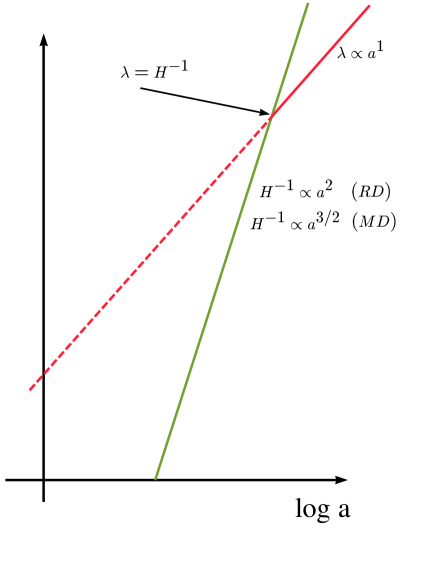
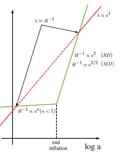
Figure 1: Physical sizes increase as $a(t)$ in the expanding universe. The Hubble radius evolves as $R_{H}=H^{-1}=(8\pi G\rho(a)/3)^{1/2}$. In a radiation-dominated or matter-dominated universe (illustrated by the left panel) any physical length scale $\lambda$ starts larger than $R_{H}$, then crosses the Hubble radius ($\lambda=H^{-1}$) only once. However, if there was a period of early inflation when $R_{H}$ increased more slowly than $a$ (as illustrated in the right panel), it is possible for a physical length scale to start smaller than $R_{H}$, become larger than $R_{H}$, and after inflation ends become once again smaller than $R_{H}$. Periods during which the scale is larger than the Hubble radius are indicated by the dotted line.

On length scales smaller than $R_{H}$ it is possible to move material around and make an imprint upon the universe. Scales larger than $R_{H}$ are “beyond the Hubble radius,” and the expansion of the universe prevents the establishment of any perturbation on scales larger than $R_{H}$.

Next consider the evolution of some physical length scale $\lambda$. Clearly, any physical length scale changes in expansion in proportion to $a(t)$.

Correlations on physical length scales $\lambda$ larger than $R_{H}(t)$ are often called acausal.

Now let us form the dimensionless ratio $L\equiv\lambda/R_{H}$. If $L$ is smaller than unity, the length scale is smaller than the Hubble radius and it is possible to imagine some microphysical process establishing perturbations on that scale, while if $L$ is larger than unity, no microphysical process can account for perturbations on that scale.

Since $R_{H}=a/\dot{a}$, and $\lambda\propto a$, the ratio $L$ is proportional to $\dot{a}$, and $\dot{L}$ scales as $\ddot{a}$, which in turn is proportional to $-(\rho+3p)$. There are two possible scenarios for $\dot{L}$ depending upon the sign of $\rho+3p$:

$$\dot{L}\ \left\{\begin{array}[]{lll}<0\rightarrow&R_{H}\mbox{ grows faster than }\lambda,&\mbox{happens for }\rho+3p>0\\ >0\rightarrow&R_{H}\mbox{ grows more slowly than }\lambda,&\mbox{happens for }\rho+3p<0.\end{array}\right.$$ (2)

In the standard MD or RD universe, $\rho+3p>0$, and $R_{H}$ grows faster than $\lambda$.

Perturbations that appear to be noncausal at last scattering can be produced if sometime during the early evolution of the universe the expansion was such that $\ddot{a}>0$. If $\ddot{a}>0$, then the Hubble radius will increase more slowly than any physical scale increases during inflation. Physical length scales larger than the Hubble radius at the time of last scattering would have been smaller than the Hubble radius during the accelerated era. Therefore it is possible to imprint correlations during inflation as a scale passes out of the horizon and have it appear as an acausal perturbation at last scattering.

From Einstein’s equations, the “acceleration” is related to the energy density and the pressure as $\ddot{a}\propto-(\rho+3p)$. Therefore, an acceleration (positive $\ddot{a}$) requires an unusual equation of state with $\rho+3p<0$. This is the condition for “accelerated expansion” or “inflation.”

We do not yet know when inflation occurred, but the best guess for the different epochs in the history of the universe is given in Table 1. It is useful to spend a few minutes discussing the movements of Table 1.

tempo	epoch	age	$\rho$	$p$	$\rho+3p$	relic
pizzicato	string dominated	$\stackrel{{\scriptstyle<}}{{{}_{\sim}}}10^{-43}$s	?	?	?	?
prestissimo	vacuum dominated (inflation)	$\sim 10^{-38}$s	$\rho_{V}$	$-\rho_{V}$	$-$	density perturbations gravitational waves dark matter?
presto	matter dominated	$\sim 10^{-36}$s	$\rho_{\phi}$	0	$+$	phase transitions? dark matter? baryogenesis?
allegro	radiation dominated	$\stackrel{{\scriptstyle<}}{{{}_{\sim}}}10^{4}$yr	$T^{4}$	$T^{4}/3$	$+$	dark matter? baryogenesis? neutrino decoupling nucleosynthesis
andante	matter dominated	$\stackrel{{\scriptstyle>}}{{{}_{\sim}}}10^{4}$yr	$\rho_{M}$	0	$+$	recombination radiation decoupling growth of structure
largo	vacuum dominated (inflation) da capo?	recent	$\rho_{V}$	$-\rho_{V}$	$-$	acceleration of the universe

Table 1: Different epochs in the history of the universe and the associated tempos of the ever decreasing expansion rate $H$, along with the equation of state and some of the relics produced during the various eras.

The first movement of the Cosmic Symphony may be dominated by the string section if on the smallest scales there is a fundamental stringiness to elementary particles. If this is true, then the first movement in the cosmic symphony would have been a pizzicato movement of vibrating strings about $10^{-43}$s after the bang. There is basically nothing known about the stringy phase, if indeed there was one. We do not yet know enough about this era to predict relics, or even the equation of state.

The earliest phase we have information about is the inflationary phase. The inflationary movement probably followed the string movement, lasting approximately $10^{-36}$ seconds. During inflation the energy density of the universe was dominated by vacuum energy, with equation of state $p_{V}\simeq-\rho_{V}$. As we shall see, the best information we have of the inflationary phase is from the quantum fluctuations during inflation, which were imprinted upon the metric, and can be observed as CBR fluctuations and the departures from homogeneity and isotropy in the matter distribution, e.g., the power spectrum. Inflation also produces a background of gravitational radiation, which can be detected by its effect on the CBR, or if inflation was sufficiently exotic, by direct detection of the relic background by experiments such as LIGO or LISA.

Inflation was wonderful, but all good things must end. A lot of effort has gone into studying the end of inflation (For a review, see Kofman et al., [2].) It was likely that there was a brief period during which the energy density of the universe was dominated by coherent oscillations of the inflaton field. During coherent oscillations the inflaton energy density scales as $a^{-3}$ where $a$ is the scale factor, so the expansion rate of the universe decreased as in a matter-dominated universe with $p\sim 0$. Very little is known about this period immediately after inflation, but there is hope that one day we will discover a relic. Noteworthy events that might have occurred during this phase include baryogenesis, phase transitions, and generation of dark matter.

We do know that the universe was radiation dominated for almost all of the first 10,000 years. The best preserved relics of the radiation-dominated era are the light elements. The light elements were produced in the radiation-dominated universe one second to three minutes after the bang. If the baryon asymmetry is associated with the electroweak transition, then the asymmetry was generated in the radiation-dominated era. The radiation era is also a likely source of dark matter such as WIMPS or axions. If one day we can detect the $1.9$ K neutrino background, it would be a direct relic of the radiation era. The equation of state during the radiation era is $p_{R}=\rho_{R}/3$.

The earliest picture of the matter-dominated era is the CBR. Recombination and matter–radiation decoupling occurred while the universe was matter dominated. Structure developed from small primordial seeds during the matter-dominated era. The pressure is negligible during the matter-dominated era.

Finally, if recent determinations of the Hubble diagram from observations of distant high-redshift Type-I supernovae are correctly interpreted, the expansion of the universe is increasing today ($\ddot{a}>0$). This would mean that the universe has recently embarked on another inflationary era, but with the Hubble expansion rate much less than the rate during the first inflationary era.

2.1 Simple Dynamics of Inflation: The Inflaton

In building inflation models it is necessary to find a mechanism by which a universe dominated by vacuum energy can make a transition from the inflationary universe to a matter-dominated or radiation-dominated universe. There is some unknown dynamics causing the expansion rate to change with time. There may be several degrees of freedom involved in determining the expansion rate during inflation, but the simplest assumption is that there is only one dynamical degree of freedom responsible for the evolution of the expansion rate.

If there is a single degree of freedom at work during inflation, then the evolution from the inflationary phase may be modeled by the action of a scalar field $\phi$ evolving under the influence of a potential $V(\phi)$. Let’s imagine the scalar field is displaced from the minimum of its potential as illustrated in Fig. 2. If the energy density of the universe is dominated by the potential energy of the scalar field $\phi$, known as the inflaton, then $\rho+3p$ will be negative. The vacuum energy disappears when the scalar field evolves to its minimum. The amount of time required for the scalar field to evolve to its minimum and inflation to end (or even more useful, the number of e-folds of growth of the scale factor) can be found by solving the classical field equation for the evolution of the inflaton field, which is simply given by $\ddot{\phi}+3H\dot{\phi}+dV/d\phi=0$.

2.2 Quantum fluctuations

In addition to the classical motion of the inflaton field, during inflation there are quantum fluctuations. Since the total energy density of the universe is dominated by the inflaton potential energy density, fluctuations in the inflaton field lead to fluctuations in the energy density. Because of the rapid expansion of the universe during inflation, these fluctuations in the energy density are frozen into super-Hubble-radius-size perturbations. Later, in the radiation or matter-dominated era they will come within the Hubble radius as if they were noncausal perturbations.

The spectrum and amplitude of perturbations depend upon the nature of the inflaton potential. Mukhanov [3] has developed a very nice formalism for the calculation of density perturbations. One starts with the action for gravity (the Einstein–Hilbert action) plus a minimally-coupled scalar inflaton field $\phi$:

$$S=-\int d^{4}\!x\ \sqrt{-g}\left[\frac{m^{2}_{Pl}}{16\pi}R-\frac{1}{2}g^{\mu\nu}\partial_{\mu}\phi\partial_{\nu}\phi+V(\phi)\right]\ .$$ (3)

Here $R$ is the Ricci curvature scalar. Quantum fluctuations result in perturbations in the metric tensor and the inflaton field

$$g_{\mu\nu}\rightarrow g_{\mu\nu}^{FRW}+\delta g_{\mu\nu}\ \ ;\qquad\phi\rightarrow\phi_{0}+\delta\phi\ ,$$ (4)

where $g_{\mu\nu}^{FRW}$ is the Friedmann–Robertson–Walker metric, and $\phi_{0}(t)$ is the classical solution for the homogeneous, isotropic evolution of the inflaton. The action describing the dynamics of the small perturbations can be written as

$$\delta_{2}S=\frac{1}{2}\int d^{4}\!x\ \left[\partial_{\mu}u\partial^{\mu}u+z^{-1}\frac{d^{2}z}{d\tau^{2}}\ u^{2}\right]\ ;\quad z=a\dot{\phi}/H\ ,$$ (5)

i.e., the action in conformal time $\tau$ ($d\tau^{2}=a^{2}(t)dt^{2})$ for a scalar field in Minkowski space, with mass-squared $m_{u}^{2}=-z^{-1}d^{2}z/d\tau^{2}$. Here, the scalar field $u$ is a combination of metric fluctuations $\delta g_{\mu\nu}$ and scalar field fluctuations $\delta\phi$. This scalar field is related to the amplitude of the density perturbation.

The simple matter of calculating the perturbation spectrum for a noninteracting scalar field in Minkowski space will give the amplitude and spectrum of the density perturbations. The problem is that the solution to the field equations depends upon the background field evolution through the dependence of the mass of the field upon $z$. Different choices for the inflaton potential $V(\phi)$ results in different background field evolutions, and hence, different spectra and amplitudes for the density perturbations.

Before proceeding, now is a useful time to remark that in addition to scalar density perturbations, there are also fluctuations in the transverse, traceless component of the spatial part of the metric. These fluctuations (known as tensor fluctuations) can be thought of as a background of gravitons.

Although the scalar and tensor spectra depend upon $V(\phi)$, for most potentials they can be characterized by $Q_{RMS}^{PS}$ (the amplitude of the scalar and tensor spectra on large length scales added in quadrature), $n$ (the scalar spectral index describing the best power-law fit of the primordial scalar spectrum), $r$ (the ratio of the tensor-to-scalar contribution to $C_{2}$ in the angular power spectrum), and $n_{T}$ ( the tensor spectral index describing the best power-law fit of the primordial tensor spectrum). For single-field, slow-roll inflation models, there is a relationship between $n_{T}$ and $r$, so in fact there are only three independent variables. Furthermore, the amplitude of the fluctuations often depends upon a free parameter in the potential, and the spectra are normalized by $Q_{RMS}^{PS}$. This leads to a characterization of a wide-range of inflaton potentials in terms of two numbers, $n$ and $r$.

2.3 Models of inflation

A quick perusal of the literature will reveal many models of inflation. Some of the familiar names to be found include: old, new, pre-owned, chaotic, quixotic, ergodic, exotic, heterotic, autoerotic, natural, supernatural, au natural, power-law, powerless, power-mad, one-field, two-field, home-field, modulus, modulo, moduli, self-reproducing, self-promoting, hybrid, low-bred, white-bread, first-order, second-order, new-world order, pre-big-bang, no-big-bang, post-big-bang, D-term, F-term, winter-term, supersymmetric, superstring, superstitious, extended, hyperextended, overextended, D-brane, p-brane, No-brain, dilaton, dilettante, $\ldots$

Probably the first step in sorting out different models is a classification scheme. One proposed classification scheme has two main types. Type-I inflation models are models based on a single inflaton field, slowly rolling under the influence of an inflaton potential $V(\phi)$. This may seem like a restrictive class, but in fact many more complicated models can be expressed in terms of an equivalent Type-I model. For instance “extended” inflation, which is a Jordan–Brans–Dicke model with an inflaton field and a JBD scalar field, can be recast as an effective Type-I model. Anything that is not Type I is denoted as a Type-II model.

Figure 2: Schematic illustrations of the inflaton potential energy. The first potential is a “large-field” model (Type-Ia). The second figure illustrates a “small-field” model (Type-Ib). The final figure illustrates an example of hybrid inflation (Type-Ic). Notice that the minimum of the potential is nonzero in the hybrid model.

There are subclasses within Type I. Type-Ia models are “large-field” models, where the inflaton field starts large and evolves toward its minimum. Examples of large-field models are chaotic inflation and power-law inflation. Type-Ib models are “small-field” models, where the inflaton field starts small and evolves to its minimum at larger values of the inflaton field. Examples of small-field models are new inflation and natural inflation. Finally, hybrid-inflation models are classified as Type-Ic models. In Type-Ia and Type-Ib models the vacuum energy is approximately zero at the end of inflation. Hybrid models have a significant vacuum energy at the end of inflation (see Fig 2). Hybrid inflation is usually terminated by a first-order phase transition or by the action of a second scalar field. A more accurate description of large-field and small-field potential is the sign of the second derivative of the potential: large-field models have $V^{\prime\prime}>0$ while small-field models have $V^{\prime\prime}<0$.

Of course a classification scheme is only reasonable if there are some observable quantities that can differentiate between different schemes. It turns out that the different Type-I models fill in different regions of the $n$–$r$ plane, as shown in Fig. 3 (from [4]). For a given spectral index $n$, small-field models have a smaller value of $r$. Shown as an ellipse is a very conservative estimate of the uncertainties in $n$ and $r$ that are expected after the next round of satellite observations. Although we don’t know where the error ellipse will fall on the graph, an error ellipse at the indicated size will restrict models. So we expect a true inflation phenomenology, where models of inflation are confronted by precision observations.

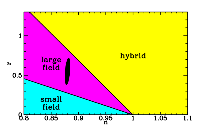
Figure 3: Large-field (Type-Ia), small-field (Type-Ib), and hybrid (Type-Ic) models seem to populate different regions of the $n$–$r$ plane. Observational determination of $n$ and $r$ could rule out entire classes of models. The dark ellipse indicated the anticipated size of the errors in the post-Planck era. Of course the location is yet to be determined. This figure is from Dodelson, Kinney and Kolb [4].

2.4 Inflation Models in the Era of Precision Cosmology

It was once said that the words “precision” and “cosmology” could not both appear in a sentence containing an even number of negatives. However that statement is now out of date, or at the very least, very soon will be out of date. A number of new instruments will come on line in the next few years and revolutionize cosmology.

There is now a world-wide campaign to pin down the microwave anisotropies. In the near future, long-duration balloon flights, as well as observations from the cold, dry observatory in Antarctica will completely change the situation. Finally, in the next decade two satellites, a NASA mission —the Microwave Anisotropy Probe (MAP)— and an ESA mission—PLANCK, will culminate in a determination of the spectrum with errors much smaller than the present errors. Of course we don’t know what the shape of the spectrum will turn out to be, but we can anticipate errors as small as shown in the figure.

With errors of this magnitude, fitting the spectrum will allow determination of $n$ and $r$, useful for inflation, as well as determination of the cosmological parameters ($H_{0}$, $\Omega_{0}$, $\Omega_{B}$, $\Lambda$, etc.) to a few percent.

2.5 Reconstruction

In addition to restricting the class of inflation models (Type Ia, Type Ib, etc.), it may be possible to use the data from precision microwave experiments to reconstruct a fragment of the inflationary potential.

Reconstruction of the inflaton potential (see Lidsey, et al., [5] for a review) refers to the process of using observational data, especially microwave background anisotropies, to determine the inflaton potential capable of generating the perturbation spectra inferred from observations [6]. Of course there is no way to prove that the reconstructed inflaton potential was the agent responsible for generating the perturbations. What can be hoped for is that one can determine a unique (within observational errors) inflaton potential capable of producing the observed perturbation spectra. The reconstructed inflaton potential may well be the first concrete piece of information to be obtained about physics at scales close to the Planck scale.

As is well known, inflation produces both scalar and tensor perturbations, and each generate microwave anisotropies (see Liddle and Lyth [7] for a review). If $V(\phi)$ is known, the perturbation spectra can be computed exactly in linear perturbation theory through integration of the relevant mode equations [8]. If the scalar field is rolling sufficiently slowly, the solutions to the mode equations may be approximated using something known as the slow-roll expansion [9, 10, 11]. The standard reconstruction program makes use of the slow-roll expansion, taking advantage of a calculation of the perturbation spectra by Stewart and Lyth [12], which gives the next-order correction to the usual lowest-order slow-roll results.

	lowest-order	next-order (exact)
$V(\phi_{*})$	$H(\phi_{*})$	$H(\phi_{*})$, $\epsilon{(\phi_{*})}$
$V^{\prime}(\phi_{*})$	$H(\phi_{*})$, $\epsilon(\phi_{*})$	$H(\phi_{*})$, $\epsilon(\phi_{*})$, $\eta(\phi_{*})$
$V^{\prime\prime}(\phi_{*})$	$H{(\phi_{*})}$, $\epsilon(\phi_{*})$, $\eta(\phi_{*})$	$H(\phi_{*})$, $\epsilon{(\phi_{*})}$, $\eta{(\phi_{*})}$, $\xi(\phi_{*})$
$V^{\prime\prime\prime}(\phi_{*})$	$H$, $\epsilon(\phi_{*})$, $\eta(\phi_{*})$, $\xi(\phi_{*})$

Table 2: A summary of the slow-roll parameters, $H$, $\epsilon$, $\eta$, and $\xi$, needed to reconstruct a given derivative of the potential to a certain order. Note that the next-order result is exact.

parameter	lowest-order	next-order
$H$	$A_{T}^{2}$	$A_{T}^{2}$, $A_{S}^{2}$
$\epsilon$	$A_{T}^{2}$, $A_{S}^{2}$	$A_{T}^{2}$, $A_{S}^{2}$, $n$
$\eta$	$A_{T}^{2}$, $A_{S}^{2}$, $n$	$A_{T}^{2}$, $A_{S}^{2}$, $n$, $dn/d\ln k$
$\xi$	$A_{T}^{2}$, $A_{S}^{2}$, $n$, $dn/d\ln k$

Table 3: The inflation parameters may be expressed in terms of the primordial scalar and tensor perturbation spectra $A_{S}^{2}$, $A_{T}^{2}$, and the scalar and tensor spectral indices $n$, and $dn/d\ln k$.

Two crucial ingredients for reconstruction are the primordial scalar and tensor perturbation spectra $A_{S}(k)$ and $A_{T}(k)$ which are defined as in Lidsey et al., [5]. The scalar and tensor perturbations depend upon the behavior of the expansion rate during inflation, which in turn depends on the value of the scaler inflaton field $\phi$. In order to track the change in the expansion rate, we define slow-roll parameters $\epsilon$, $\eta$, and $\xi$ as

$$\epsilon(\phi)\equiv\frac{m_{{\rm Pl}}^{2}}{4\pi}\left[\frac{H^{\prime}(\phi)}{H(\phi)}\right]^{2}\qquad\eta(\phi)\equiv\frac{m_{{\rm Pl}}^{2}}{4\pi}\frac{H^{\prime\prime}(\phi)}{H(\phi)}\qquad\xi(\phi)\equiv\frac{m_{{\rm Pl}}^{2}}{4\pi}\left(\frac{H^{\prime}(\phi)H^{\prime\prime\prime}(\phi)}{H^{2}(\phi)}\right)^{1/2}\ ,$$ (6)

where here the prime superscript implies $d/d\phi$. If the slow-roll parameters are small, $\epsilon$, $\eta$, and $\xi$ can be expressed in terms of derivatives of the inflaton potential:

$$\epsilon(\phi)=\frac{m_{{\rm Pl}}^{2}}{16\pi}\left(\frac{V^{\prime}}{V}\right)^{2}\qquad\eta(\phi)=\frac{m_{{\rm Pl}}^{2}}{8\pi}\,\frac{V^{\prime\prime}}{V}\qquad\xi^{2}(\phi)=\left(\frac{m^{2}_{{\rm Pl}}}{8\pi}\right)^{2}\,\frac{V^{\prime}V^{{}^{\prime\prime\prime}}}{V^{2}}\ .$$ (7)

As long as the slow-roll parameters are small compared to unity, the scalar and tensor perturbation amplitudes $A_{S}(k)$ and $A_{T}(k)$ are given by (see Stewart and Lyth [12] for the normalization)

$$A_{S}^{2}(k) \simeq \frac{4}{25\pi}\left(\frac{H}{m_{{\rm Pl}}}\right)^{2}\epsilon^{-1}\left[1-(2C+1)\epsilon+C\eta\right]^{2}$$ (8)

$$A_{T}^{2}(k) \simeq \frac{4}{25\pi}\left(\frac{H}{m_{{\rm Pl}}}\right)^{2}\left[1-(C+1)\epsilon\right]^{2}\ ,$$ (9)

where $H$, $\epsilon$, and $\eta$ are to be determined at the value of $\phi$ when $k=aH$ during inflation, and where $C=-2+\ln 2+\gamma\simeq-0.73$ is a numerical constant, $\gamma$ being the Euler constant. These equations are the basis of the reconstruction process.

From the expressions for $A_{S}^{2}$ and $A_{T}^{2}$ one can express the scalar and tensor spectral indices, defined as

$$n(k)-1\equiv\frac{d\ln A_{S}^{2}}{d\ln k}\qquad n_{T}(k)=\frac{d\ln A_{T}^{2}}{d\ln k}\,$$ (10)

in terms of slow-roll parameters.

	lowest-order	next-order	next-to-next-order
$V$	$R_{*}$, $Q_{RMS}^{PS}$	$R_{*}$, $Q_{RMS}^{PS}$	$R_{*}$, $Q_{RMS}^{PS}$, $n_{*}$
$V^{\prime}$	$R_{*}$, $Q_{RMS}^{PS}$	$R_{*}$, $Q_{RMS}^{PS}$, $n_{*}$	$R_{*}$, $Q_{RMS}^{PS}$, $n_{*}$, $n_{*}^{\prime}$
$V^{\prime\prime}$	$R_{*}$, $Q_{RMS}^{PS}$, $n_{*}$	$R_{*}$, $Q_{RMS}^{PS}$, $n_{*}$, $n_{*}^{\prime}$
$V^{\prime\prime\prime}$	$R_{*}$, $Q_{RMS}^{PS}$, $n_{*}$, $n_{*}^{\prime}$

Table 4: A summary of the observables needed to reconstruct a given derivative of the potential to a certain order. $R_{*}$ is the ratio of the tensor to scalar contributions to the CBR anisotropies at any conveniently chosen scale. $Q_{RMS}^{PS}$ is the normalization of the total (scalar plus tensor) contributions at small $l$, $n_{*}$ and $n_{*}^{\prime}$ refer to the scalar spectral index and its derivative at some scale. Knowledge of $R_{*}$ and $Q_{RMS}^{PS}$ is equivalent to determination of $A_{T}^{2}(k_{*})$ and $A_{S}^{2}(k_{*})$.

Perturbative reconstruction requires that one fits an expansion, usually a Taylor series of the form

$$\ln A_{S}^{2}(k)=\ln A_{S}^{2}(k_{*})+(n_{*}-1)\ln\frac{k}{k_{*}}+\frac{1}{2}\,\left.\frac{dn}{d\ln k}\right|_{*}\ln^{2}\!\frac{k}{k_{*}}+\frac{1}{6}\left.\frac{d^{2}n}{d(\ln k)^{2}}\right|_{*}\ln^{3}\!\frac{k}{k_{*}}+\cdots\,,$$ (11)

where $n_{*}=n(k_{*})$, to the observed spectrum in order to extract the coefficients, where stars indicate the value at $k_{*}$. The scale $k_{*}$ is most wisely chosen to be at the (logarithmic) center of the data, about $k_{*}=0.01\,h$ Mpc^-1.

For reconstruction, one takes a Hamilton–Jacobi approach where the expansion rate is considered fundamental, and the expansion rate is parameterized by a value of the inflaton field. The Friedmann equation may be expressed in terms of the potential $V(\phi)$, the expansion rate $H(\phi)$, and the derivative of $H$ as

$$\left(\frac{dH}{d\phi}\right)^{2}-\frac{12\pi}{M_{Pl}^{2}}H^{2}=-\frac{32\pi^{2}}{m_{Pl}^{4}}V(\phi)$$ (12)

or equivalently in terms of the slow-roll parameter $\epsilon$, as

$$V=\frac{m_{Pl}^{2}H^{2}}{8\pi}(3-\epsilon)\ .$$ (13)

Subsequent derivatives of $V$ may be expressed in terms of additional slow-roll parameters:

$$V^{\prime}=-\frac{m_{Pl}^{2}}{\sqrt{4\pi}}\,H^{2}\epsilon^{1/2}(3-\eta)\qquad V^{\prime\prime}=H^{2}\left(3\epsilon+3\eta-\eta^{2}+\xi^{2}\right)\ ,$$ (14)

and so on. So if one can determine the slow-roll parameters, one has information about the potential. The slow-roll parameters needed to reconstruct a given derivative of the potential is given in Table 2.

Of course, the problem is that the slow-roll parameters are not directly observable! But one can construct an iterative scheme to express the slow-roll parameters in terms of observables. The result is shown in Table 3.

Using the notation $n^{\prime}_{*}$ to indicate $\left.dn/d\ln k\right|_{*}$ and $R_{*}=A_{T}^{2}(k_{*})/A_{S}^{2}(k_{*})$, the reconstruction equations are

$$m_{{\rm Pl}}^{-4}\,V(\phi_{*}) \simeq \frac{75}{32}A_{S}^{2}(k_{*})R_{*}\left\{\phantom{\frac{1}{2}}\!\!\!\!1+\left[0.21R_{*}\right]\,\right\}$$

$$m_{{\rm Pl}}^{-3}\,V^{\prime}(\phi_{*}) \simeq -\frac{75\sqrt{\pi}}{8}A_{S}^{2}(k_{*})R_{*}^{3/2}\left\{1\phantom{\frac{1}{2}}\!\!\!\!-\left[\phantom{R_{*}^{2}}\!\!\!\!\!\!\!0.85R_{*}-0.53(1-n_{*})\right]\,\right\}$$

$$m_{{\rm Pl}}^{-2}\,V^{\prime\prime}(\phi_{*}) \simeq \frac{25\pi}{4}A_{S}^{2}(k_{*})R_{*}\left\{9R_{*}-1.5(1-n_{*})\phantom{\frac{1}{2}}\!\!\!\!\right.-\left[24.3R_{*}^{2}+0.25(1-n_{*})^{2}\right.$$ (15)

$$\!\!\!\!\!\!\!\!\!\!\left.\phantom{\frac{1}{2}}\left.\phantom{R_{*}^{2}}-14.8R_{*}(1-n_{*})-1.6\,n^{\prime}_{*}\right]\right\}\,.$$

The observables needed to reconstruct a given derivation of the potential are listed in Table 4.

The biggest hurdle for successful reconstruction is that many inflation models predict a tensor perturbation amplitude (hence, $R_{*}$) well below the expected threshold for detection, and even above detection threshold the errors can be considerable. If the tensor modes cannot be identified a unique reconstruction is impossible, as the scalar perturbations are governed not only by $V(\phi)$, but by the first derivative of $V(\phi)$ as well. Knowledge of only the scalar perturbations leaves an undetermined integration constant in the non-linear system of reconstruction equations. Another problem is that simple potentials usually lead to a nearly exact power-law scalar spectrum with the spectral index close to unity. In such a scenario only a very limited amount of information could be obtained about high energy physics from astrophysical observations.

However if a tensor mode can be determined, then one may follow the following reconstruction procedure. $R_{*}$, $n_{*}$, $n^{\prime}_{*}$, $\ldots$ are to be determined from observations. Fortunately, parameter estimation from the microwave background has been explored in some detail [13, 14]. We shall use error estimates for Planck assuming polarized detectors are available, following the analysis of Zaldarriaga et al., [14]. Most analyses have assumed that $R_{*}$ and $n_{*}$ are the only parameters needed to describe the spectra. In a recent paper [15], Copeland, Grivell, and Liddle have generalized their treatment to allow the power spectrum to deviate from scale-invariance. Including extra parameters leads to a deterioration in the determination of all the parameters, as it introduces extra parameter degeneracies. Fortunately, for most parameters the uncertainty is not much increased by including the first few derivatives of $n$ [15], but the parameter $n$ itself has a greatly increased error bar. If a power-law is assumed it can be determined to around $\Delta n\simeq 0.004$ [14, 15], but including scale dependence increases this error bar by a factor of ten or more. Notice that unless one assumes a perfect power-law behavior, this increase in uncertainty is applicable even if the deviation from power-law behavior cannot be detected within the uncertainty.

From Grivell and Liddle [8], an estimate of the relevant uncertainties is

$$\Delta(R_{*})\simeq 0.004\;\; \;\;\Delta(dn/d\ln k)\simeq 0.04$$ ;

$$\Delta n\simeq 0.15\;\; \;\;\Delta[d^{2}n/d(\ln k)^{2}]\simeq 0.005\,.$$ ; (16)

Once $R_{*}$, $A_{S}^{2}$, $n_{*}$, and $n^{\prime}_{*}$ are determined, then it is possible to find $V(\phi_{*})$, $V^{\prime}(\phi_{*})$, and $V^{\prime\prime}(\phi_{*})$ from Eq. 2.5. Then one can express $V(\phi)$ as a Taylor series about $V(\phi_{*})$:

$$V(\phi)=V(\phi_{*})+V^{\prime}(\phi_{*})\Delta\phi+\frac{1}{2}V^{\prime\prime}(\phi_{*})\Delta\phi^{2}+\cdots\ .$$ (17)

$\Delta\phi$ is found from an exact expression connecting changes in $\phi$ with changes in $k$ [5],

$$\frac{d\phi}{d\ln k}=\frac{m_{{\rm Pl}}^{2}}{4\pi}\frac{H^{\prime}}{H}\frac{1}{\epsilon-1}\simeq\sqrt{\frac{R_{*}}{4\pi}}\,(1+R_{*})\,.$$ (18)

Let me illustrate reconstruction by considering two sample potentials. The first potential, discussed by Lidsey et al., [5] is a power-law potential, $V(\phi)=V_{0}\exp(-\alpha\phi/m_{Pl})$, with $\alpha\simeq 1.6$. The potential is shown in the upper left-hand-side of Fig. 4. This potential generates a spectral index of $n_{*}=0.9$ and $n^{\prime}_{*}=0$. It also results in a value of $R_{*}=0.1$. So one might guess that precision CBR measurements will determine $R_{*}$, $n_{*}$, and $n^{\prime}_{*}$ of these values, with uncertainties of Eq. 2.5.

In order to see what sort of reconstructed potential results, one can imagine a model universe with $R_{*}$, $n_{*}$, and $n^{\prime}_{*}$ generated as Gaussian random variables with mean determined by the underlying potential and variance determined by the expected observational uncertainties. The result of ten such reconstructions of the potential are shown in the upper left-hand figure of Fig. 4. The range of $\phi$ is determined by the range of wavenumber over which one expects to have accurate determinations of the parameters from the CBR. Here $k_{*}$ was chosen to be $0.01h$ Mpc^-1 and the range of $k$ taken to be three decades.

Also shown in Fig. 4 in the upper right-hand panel is information about the reconstruction of the first derivative of the potential.

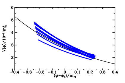
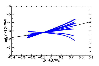
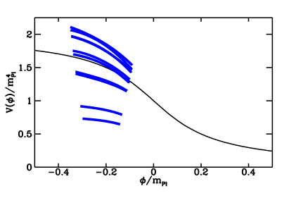
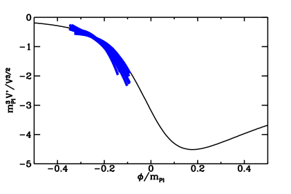
Figure 4: Sample reconstructions of two inflationary potentials. The upper two figures are the reconstruction of a power-law potential of the form $V(\phi)=V_{0}\exp(-\alpha\phi/m_{Pl})$. The light curves are from the true potential, while the heavy curves are ten reconstructions. The lower figures are the actual potential and ten reconstructions of a potential of the form $V(\phi)=\Lambda^{4}[1-(2/\pi)\tan^{-1}(5\phi/m_{\rm Pl})]$.

The second example of reconstruction was considered in Copeland et al., [16] The potential, first considered by Wang et al., [17] is a potential of the form

$$V(\phi)=\Lambda^{4}\left(1-\frac{2}{\pi}\,\tan^{-1}\frac{5\phi}{m_{{\rm Pl}}}\right)\,,$$ (19)

which is shown in the lower left-hand side of Fig. 4.

A fit to a Taylor expansion to the exact spectrum, using $k_{*}$ as above, yields the following results:

$$\ln A_{S}^{2}(k_{*})=3.84\quad;\quad R_{*}=0.014\quad;n_{*}=0.579\quad;\quad$$

$$\left.\frac{dn}{d\ln k}\right|_{*}=-0.134\left.\frac{d^{2}n}{d(\ln k)^{2}}\right|_{*}=-0.052\ .$$ (20)

From the estimated observational uncertainties of Eq. (2.5), we see that all these coefficients should be successfully determined at high significance and a simple “chi–by–eye” demonstrates that the spectrum reconstructed from these data is an adequate fit to the observed spectrum. This stresses the point that the more unusual a potential is, the more information one is likely to be able to extract about it, though the uncertainties on the individual pieces of information may be greater.

We reconstruct the potential in a region about $\phi_{*}=-0.22$ (the reconstruction program does not determine $\phi_{*}$), the width of the region given via Eq. (18). The result for the reconstructed potential including the effect of observational errors and cosmic variance are shown in Fig. 4, where it can immediately be seen that the reconstruction has been very successful in reproducing the main features of the potential while perturbations on interesting scales are being developed.

The uncertainty is dominated by that of $A_{T}^{2}(k_{*})$; although the gravitational waves are detectable in this model, it is only about a three-sigma detection and the error bar is thus large. Since the overall magnitude of the potential is proportional to $A_{T}^{2}$, the visual impression is of a large uncertainty.

Fortunately, information in combinations of the higher derivatives is more accurately determined. Fig. 4 also shows the reconstruction of $V^{\prime}/V^{3/2}$ with observational errors; this combination is chosen as it is independent of the tensors to lowest order. Not only is it reconstructed well at the central point, but both the gradient and curvature are well fit too, confirming useful information has been obtained about not just $V^{\prime\prime}$ but $V^{\prime\prime\prime}$ as well, which is only possible because of the extra information contained in the scale-dependence of the power spectrum. So rather accurate information is being obtained about the potential.

3 Preheating, Reheating, and Dark Matter

If the inflaton is completely decoupled, then once inflation ends it will oscillate about the minimum of the potential, with the cycle-average of the energy density decreasing as $a^{-3}$, i.e., as a matter-dominated universe. But at the end of inflation the universe is cold and frozen in a low-entropy state: the only degree of freedom is the zero-momentum mode of the inflaton field. It is necessary to “defrost” the universe and turn it into a “hot” high-entropy universe with many degrees of freedom in the radiation. Exactly how this is accomplished is still unclear. It probably requires the inflaton field to be coupled to other degrees of freedom, and as it oscillates, its energy is converted to radiation either through incoherent decay, or through a coherent process involving very complicated dynamics of coupled oscillators with time-varying masses. In either case, it is necessary to extract the energy from the inflaton and convert it into radiation.

I will now turn to a discussion of how defrosting might occur. It may be a complicated several-step process. I will refer to nonlinear effects in defrosting as “preheating” [2] and refer to linear processes as “reheating” [18].

The possible role of nonlinear dynamics leading to explosive particle production has recently received a lot of attention. This process, known as “preheating” [2] may convert a fair fraction of the inflaton energy density into other degrees of freedom, with extremely interesting cosmological effects such as symmetry restoration, baryogenesis, or production of dark matter. But the efficiency of preheating is very sensitive to the model and the model parameters.

Perhaps some relic of defrosting, such as symmetry restoration, baryogenesis, or dark matter may provide a clue of the exact mechanism, and even shed light on inflation.

3.1 Defrosting the Universe After Inflation

3.1.1 Reheating

In one extreme is the assumption that the vacuum energy of inflation is immediately converted to radiation resulting in a reheat temperature $T_{RH}$.

A second (and more plausible) scenario is that reheating is not instantaneous, but is the result of the slow decay of the inflaton field. The simplest way to envision this process is if the comoving energy density in the zero mode of the inflaton decays into normal particles, which then scatter and thermalize to form a thermal background. It is usually assumed that the decay width of this process is the same as the decay width of a free inflaton field.

There are two reasons to suspect that the inflaton decay width might be small. The requisite flatness of the inflaton potential suggests a weak coupling of the inflaton field to other fields since the potential is renormalized by the inflaton coupling to other fields [19]. However, this restriction may be evaded in supersymmetric theories where the nonrenormalization theorem ensures a cancellation between fields and their superpartners. A second reason to suspect weak coupling is that in local supersymmetric theories gravitinos are produced during reheating. Unless reheating is delayed, gravitinos will be overproduced, leading to a large undesired entropy production when they decay after big-bang nucleosynthesis [20].

With the above assumptions, the Boltzmann equations describing the redshift and interchange in the energy density among the different components is

$$\dot{\rho}_{\phi}+3H\rho_{\phi}+\Gamma_{\phi}\rho_{\phi}=0$$

$$\dot{\rho}_{R}+4H\rho_{R}-\Gamma_{\phi}\rho_{\phi}=0\ ,$$ (21)

where dot denotes time derivative. The dynamics of reheating will be discussed in detail in Section 3.2.3.

The reheat temperature is calculated quite easily [18]. After inflation the inflaton field executes coherent oscillations about the minimum of the potential. Averaged over several oscillations, the coherent oscillation energy density redshifts as matter: $\rho_{\phi}\propto a^{-3}$, where $a$ is the Robertson–Walker scale factor. If we denote as $\rho_{I}$ and $a_{I}$ the total inflaton energy density and the scale factor at the initiation of coherent oscillations, then the Hubble expansion rate as a function of $a$ is ($M_{Pl}$ is the Planck mass)

$$H(a)=\sqrt{\frac{8\pi}{3}\frac{\rho_{I}}{M^{2}_{Pl}}\left(\frac{a_{I}}{a}\right)^{3}}\ .$$ (22)

Equating $H(a)$ and $\Gamma_{\phi}$ leads to an expression for $a_{I}/a$. Now if we assume that all available coherent energy density is instantaneously converted into radiation at this value of $a_{I}/a$, we can define the reheat temperature by setting the coherent energy density, $\rho_{\phi}=\rho_{I}(a_{I}/a)^{3}$, equal to the radiation energy density, $\rho_{R}=(\pi^{2}/30)g_{*}T_{RH}^{4}$, where $g_{*}$ is the effective number of relativistic degrees of freedom at temperature $T_{RH}$. The result is

$$T_{RH}=\left(\frac{90}{8\pi^{3}g_{*}}\right)^{1/4}\sqrt{\Gamma_{\phi}M_{Pl}}\ =0.2\left(\frac{200}{g_{*}}\right)^{1/4}\sqrt{\Gamma_{\phi}M_{Pl}}\ .$$ (23)

The limit from gravitino overproduction is $T_{RH}\stackrel{{\scriptstyle<}}{{{}_{\sim}}}10^{9}$ to $10^{10}$ GeV.

3.1.2 Preheating

The main ingredient of the preheating scenario introduced in the early 1990s is the nonperturbative resonant transfer of energy to particles induced by the coherently oscillating inflaton fields. It was realized that this nonperturbative mechanism can be much more efficient than the usual perturbative mechanism for certain parameter ranges of the theory [21].

The basic picture can be seen as follows. Assume there is an inflaton field $\phi$ oscillating about the minimum of a potential $V(\phi)=m^{2}\phi^{2}/2$. It is convenient to parameterize the motion of the inflaton field as

$$\phi(t)=\Phi(t)\sin mt.$$ (24)

In an expanding universe, even in the absence if interactions the amplitude of the oscillations of the inflaton field, $\Phi$, decreases slowly due to the redshift of the momentum. In Minkowski space, $\Phi$ would be a constant in the absence of interactions..

Suppose there is a scalar field $X$ with a coupling to the inflaton of $g^{2}\phi^{2}X^{2}/2$. The mode equation for the $X$ field can be written in terms of a redefined variable $\chi_{k}\equiv X_{k}a^{3/2}$ as

$$\ddot{\chi}_{k}+3\frac{\dot{a}}{a}\chi_{k}+\left[\frac{{\rm\bf k}^{2}}{a^{2}}+g^{2}\Phi^{2}(t)\sin^{2}(mt)\right]\chi_{k}=0\ .$$ (25)

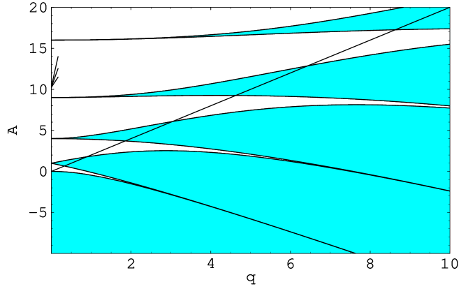
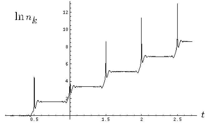
Figure 5: Shaded areas are regions of explosive particle production. The line is $A_{k}=2q$ (recall $A_{k}=2q+k^{2}/m^{2}$). This figure is from Chung [22].

Figure 6: Explosive particle production if $A_{k}$ and $q$ are constant. This figure is from Kofman, Linde, and Starobinski [2].

In Minkowski space $\dot{a}/a=0$ and $\Phi(t)$ is constant, and the mode equation becomes (prime denotes $d/dz$ where $z=mt$)

$$\chi^{\prime\prime}_{k}+[A_{k}-2q\cos(2z)]\chi_{k}(t)=0\ .$$ (26)

The parameter $q$ depends on the inflaton field oscillation amplitude, and $A_{k}$ depends on the energy of the particle and $q$:

$$q = \frac{g^{2}\Phi^{2}}{4m^{2}}$$

$$A_{k} = 2q+\frac{k^{2}}{m^{2}}\ .$$ (27)

When $A_{k}$ and $q$ are constants, the equation is the Mathieu equation, which exhibits resonant mode instabilities for certain values of $A_{k}$ and $q$. If $A_{k}$ and $q$ are constant, then there are instability regions where there is explosive particle production. The instability regions are shown in Fig. 6 from the paper of Chung [22].

Integration of the field equations for the number of particles created in a particular $k$ mode is shown in Fig. 6. Explosive growth occurs every time the inflaton passes through the origin.

In an expanding universe, $A_{k}$ and $q$ will vary in time, but if they vary slowly compared to the frequency of oscillations, the effects of resonance will remain. An example of particle production where $A_{k}$ and $q$ vary due to expansion is shown in Fig. 7. Details of the parameters and the calculation can be found in Kofman, Linde, and Starobinski [2].

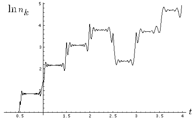
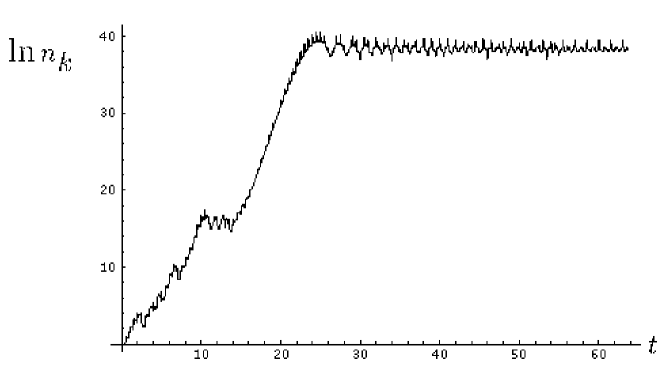
Figure 7: Explosive particle production if $A_{k}$ and $q$ are not constant. The lower figure shows integration for a longer time. These figures are from Kofman, Linde, and Starobinski [2].

If the mode occupation number for the $X$ particles is large, the number density per mode of the $X$ particles will be proportional to $|\chi_{k}|^{2}$. If $A_{k}$ and $q$ have the appropriate values for resonance, $\chi_{k}$ will grow exponentially in time, and hence the number density will attain an exponential enhancement above the usual perturbative decay. This period of enhanced rate of energy transfer has been called preheating primarily because the particles that are produced during this period have yet to achieve thermal equilibrium.

This resonant amplification leads to an efficient transfer of energy from the inflaton to other particles which may have stronger coupling to other particles than the inflaton, thereby speeding up the reheating process and leading to a higher reheating temperature than in the usual scenario.

One possible result of preheating is a phase transition caused by the large number of soft particles created in preheating [23].

Another interesting feature is that particles of mass larger than the inflaton mass can be produced through this coherent resonant effect. This has been exploited to construct a baryogenesis scenario [24] in which the baryon number violating bosons with masses larger than the inflaton mass are created through the resonance mechanism.

3.2 Dark Matter

There are many reasons to believe the present mass density of the universe is dominated by a weakly interacting massive particle (wimp), a fossil relic of the early universe. Theoretical ideas and experimental efforts have focused mostly on production and detection of thermal relics, with mass typically in the range a few GeV to a hundred GeV. Here, I will review scenarios for production of nonthermal dark matter. Since the masses of the nonthermal wimps are in the range $10^{12}$ to $10^{19}$ GeV, much larger than the mass of thermal wimpy wimps, they may be referred to as wimpzillas. In searches for dark matter it may be well to remember that “size does matter.”

3.2.1 Thermal Relics—Wimpy WIMPS

It is usually assumed that the dark matter consists of a species of a new, yet undiscovered, massive particle, traditionally denoted by $X$. It is also often assumed that the dark matter is a thermal relic, i.e., it was in chemical equilibrium in the early universe.

A thermal relic is assumed to be in local thermodynamic equilibrium (lte) at early times. The equilibrium abundance of a particle, say relative to the entropy density, depends upon the ratio of the mass of the particle to the temperature. Define the variable $Y\equiv n_{X}/s$, where $n_{X}$ is the number density of WIMP $X$ with mass $M_{X}$, and $s\sim T^{3}$ is the entropy density. The equilibrium value of $Y$, $Y_{EQ}$, is proportional to $\exp(-x)$ for $x\gg 1$, while $Y_{EQ}\sim$ constant for $x\ll 1$, where $x=M_{X}/T$.

A particle will track its equilibrium abundance as long as reactions which keep the particle in chemical equilibrium can proceed rapidly enough. Here, rapidly enough means on a timescale more rapid than the expansion rate of the universe, $H$. When the reaction rate becomes smaller than the expansion rate, then the particle can no longer track its equilibrium value, and thereafter $Y$ is constant. When this occurs the particle is said to be “frozen out.” A schematic illustration of this is given in Fig. 8.

Figure 8: A thermal relic starts in lte at $T\gg M_{X}$. When the rates keeping the relic in chemical equilibrium become smaller than the expansion rate, the density of the relic relative to the entropy density freezes out.

The more strongly interacting the particle, the longer it stays in lte, and the smaller its eventual freeze-out abundance. Conversely, the more weakly interacting the particle, the larger its present abundance. The freeze-out value of $Y$ is related to the mass of the particle and its annihilation cross section (here characterized by $\sigma_{0}$) by [18]

$$Y\propto\frac{1}{M_{X}m_{Pl}\sigma_{0}}\ .$$ (28)

Since the contribution to $\Omega$ is proportional to $M_{X}n_{X}$, which in turn is proportional to $M_{X}Y$, the present contribution to $\Omega$ from a thermal relic roughly is independent of its mass, and depends only upon the annihilation cross section. The cross section that results in $\Omega_{X}h^{2}\sim 1$ is of order $10^{-37}$cm², i.e., of the order of the weak scale. This is one of the attractions of thermal relics. The scale of the annihilation cross section is related to a known mass scale.

The simple assumption that dark matter is a thermal relic is surprisingly restrictive. The largest possible annihilation cross section is roughly $M_{X}^{-2}$. This implies that large-mass wimps would have such a small annihilation cross section that their present abundance would be too large. Thus one expects a maximum mass for a thermal WIMP, which turns out to be a few hundred TeV [25].

The standard lore is that the hunt for dark matter should concentrate on particles with mass of the order of the weak scale and with interaction with ordinary matter on the scale of the weak force. This has been the driving force behind the vast effort in dark matter direct detection.

In view of the unitarity argument, in order to consider thermal wimpzillas, one must invoke, for example, late-time entropy production to dilute the abundance of these supermassive particles [26], rendering the scenario unattractive.

3.2.2 Nonthermal Relics—WIMPZILLAS

There are two necessary conditions for the wimpzilla scenario. First, the wimpzilla must be stable, or at least have a lifetime much greater than the age of the universe. This may result from, for instance, supersymmetric theories where the breaking of supersymmetry is communicated to ordinary sparticles via the usual gauge forces [27]. In particular, the secluded and the messenger sectors often have accidental symmetries analogous to baryon number. This means that the lightest particle in those sectors might be stable and very massive if supersymmetry is broken at a large scale [28]. Other natural candidates arise in theories with discrete gauge symmetries [29] and in string theory and M theory [30, 31].

It is useful here to note that wimpzilla decay might be able to account for ultra-high energy cosmic rays above the Greisen–Zatzepin–Kuzmin cutoff [32, 33]. A wimpy little thermal relic would be too light to do the job, a wimpzilla is needed.

The second condition for a wimpzilla is that it must not have been in equilibrium when it froze out (i.e., it is not a thermal relic), otherwise $\Omega_{X}h^{2}$ would be much larger than one. A sufficient condition for nonequilibrium is that the annihilation rate (per particle) must be smaller than the expansion rate: $n_{X}\sigma|v|<H$, where $\sigma|v|$ is the annihilation rate times the Møller flux factor, and $H$ is the expansion rate. Conversely, if the dark matter was created at some temperature $T_{*}$ and $\Omega_{X}h^{2}<1$, then it is easy to show that it could not have attained equilibrium. To see this, assume $X$’s were created in a radiation-dominated universe at temperature $T_{*}$. Then $\Omega_{X}h^{2}$ is given by

$$\Omega_{X}h^{2}=\Omega_{\gamma}h^{2}(T_{*}/T_{0})m_{X}n_{X}(T_{*})/\rho_{\gamma}(T_{*})\ ,$$ (29)

where $T_{0}$ is the present temperature. Using the fact that $\rho_{\gamma}(T_{*})=H(T_{*})M_{Pl}T_{*}^{2}$, $n_{X}(T_{*})/H(T_{*})=(\Omega_{X}/\Omega_{\gamma})T_{0}M_{Pl}T_{*}/M_{X}$. One may safely take the limit $\sigma|v|<M_{X}^{-2}$, so $n_{X}(T_{*})\sigma|v|/H(T_{*})$ must be less than $(\Omega_{X}/\Omega_{\gamma})T_{0}M_{Pl}T_{*}/M_{X}^{3}$. Thus, the requirement for nonequilibrium is

$$\left(\frac{200\,{\rm TeV}}{M_{X}}\right)^{2}\left(\frac{T_{*}}{M_{X}}\right)<1\ .$$ (30)

This implies that if a nonrelativistic particle with $M_{X}\stackrel{{\scriptstyle>}}{{{}_{\sim}}}200$ TeV was created at $T_{*}<M_{X}$ with a density low enough to result in $\Omega_{X}\stackrel{{\scriptstyle<}}{{{}_{\sim}}}1$, then its abundance must have been so small that it never attained equilibrium. Therefore, if there is some way to create wimpzillas in the correct abundance to give $\Omega_{X}\sim 1$, nonequilibrium is automatic. Examples of wimpzilla evolution and freezeout are shown in Fig. 9.

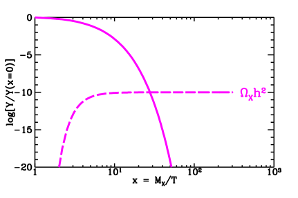
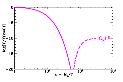
Figure 9: A nonthermal relic typically has abundance much less than lte at $T\gg M_{X}$. Here are two examples of the evolution of a nonthermal relic. In the left panel $Y\ll Y_{EQ}$ at freezeout, while in the right panel $Y\gg Y_{EQ}$ at freezeout. Again, the solid curve is the lte abundance while the dashed curve is the actual abundance.

Any wimpzilla production scenario must meet these two criteria. Before turning to several wimpzilla production scenarios, it is useful to estimate the fraction of the total energy density of the universe in wimpzillas at the time of their production that will eventually result in $\Omega\sim 1$ today.

The most likely time for wimpzilla production is just after inflation. The first step in estimating the fraction of the energy density in wimpzillas is to estimate the total energy density when the universe is “reheated” after inflation.

Consider the calculation of the reheat temperature, denoted as $T_{RH}$. The reheat temperature is calculated by assuming an instantaneous conversion of the energy density in the inflaton field into radiation when the decay width of the inflaton energy, $\Gamma_{\phi}$, is equal to $H$, the expansion rate of the universe. The derivation of the reheat temperature was given in Section 3.1.1.

Now consider the wimpzilla density at reheating. Suppose the wimpzilla never attained lte and was nonrelativistic at the time of production. The usual quantity $\Omega_{X}h^{2}$ associated with the dark matter density today can be related to the dark matter density when it was produced. First write

$$\frac{\rho_{X}(t_{0})}{\rho_{R}(t_{0})}=\frac{\rho_{X}(t_{RH})}{\rho_{R}(t_{RH})}\>\left(\frac{T_{RH}}{T_{0}}\right),$$ (31)

where $\rho_{R}$ denotes the energy density in radiation, $\rho_{X}$ denotes the energy density in the dark matter, $T_{RH}$ is the reheat temperature, $T_{0}$ is the temperature today, $t_{0}$ denotes the time today, and $t_{RH}$ denotes the approximate time of reheating. To obtain $\rho_{X}(t_{RH})/\rho_{R}(t_{RH})$, one must determine when $X$ particles are produced with respect to the completion of reheating and the effective equation of state between $X$ production and the completion of reheating.

At the end of inflation the universe may have a brief period of matter domination resulting either from the coherent oscillations phase of the inflaton condensate or from the preheating phase [21]. If the $X$ particles are produced at time $t=t_{e}$ when the de Sitter phase ends and the coherent oscillation period just begins, then both the $X$ particle energy density and the inflaton energy density will redshift at approximately the same rate until reheating is completed and radiation domination begins. Hence, the ratio of energy densities preserved in this way until the time of radiation domination is

$$\frac{\rho_{X}(t_{RH})}{\rho_{R}(t_{RH})}\approx\frac{8\pi}{3}\>\frac{\rho_{X}(t_{e})}{M_{Pl}^{2}H^{2}(t_{e})},$$ (32)

where $M_{Pl}\approx 10^{19}$ GeV is the Planck mass and most of the energy density in the universe just before time $t_{RH}$ is presumed to turn into radiation. Thus, using Eq. 31, one may obtain an expression for the quantity $\Omega_{X}\equiv\rho_{X}(t_{0})/\rho_{C}(t_{0})$, where $\rho_{C}(t_{0})=3H_{0}^{2}M_{Pl}^{2}/8\pi$ and $H_{0}=100\>h$ km sec^-1 Mpc^-1:

$$\Omega_{X}h^{2}\approx\Omega_{R}h^{2}\>\left(\frac{T_{RH}}{T_{0}}\right)\>\frac{8\pi}{3}\left(\frac{M_{X}}{M_{Pl}}\right)\>\frac{n_{X}(t_{e})}{M_{Pl}H^{2}(t_{e})}.$$ (33)

Here $\Omega_{R}h^{2}\approx 4.31\times 10^{-5}$ is the fraction of critical energy density in radiation today and $n_{X}$ is the density of $X$ particles at the time when they were produced.

Note that because the reheating temperature must be much greater than the temperature today ($T_{RH}/T_{0}\stackrel{{\scriptstyle>}}{{{}_{\sim}}}4.2\times 10^{14}$), in order to satisfy the cosmological bound $\Omega_{X}h^{2}\stackrel{{\scriptstyle<}}{{{}_{\sim}}}1$, the fraction of total wimpzilla energy density at the time when they were produced must be extremely small. One sees from Eq. 33 that $\Omega_{X}h^{2}\sim 10^{17}(T_{RH}/10^{9}\mbox{GeV})(\rho_{X}(t_{e})/\rho(t_{e}))$. It is indeed a very small fraction of the total energy density extracted in wimpzillas.

This means that if the wimpzilla is extremely massive, the challenge lies in creating very few of them. Gravitational production discussed in Section 3.2.3 naturally gives the needed suppression. Note that if reheating occurs abruptly at the end of inflation, then the matter domination phase may be negligibly short and the radiation domination phase may follow immediately after the end of inflation. However, this does not change Eq. 33.

3.2.3 Wimpzilla Production

3.2.3.a Gravitational Production

First consider the possibility that wimpzillas are produced in the transition between an inflationary and a matter-dominated (or radiation-dominated) universe due to the “nonadiabatic” expansion of the background spacetime acting on the vacuum quantum fluctuations [34].

The distinguishing feature of this mechanism is the capability of generating particles with mass of the order of the inflaton mass (usually much larger than the reheating temperature) even when the particles only interact extremely weakly (or not at all) with other particles and do not couple to the inflaton. They may still be produced in sufficient abundance to achieve critical density today due to the classical gravitational effect on the vacuum state at the end of inflation. More specifically, if $0.04\stackrel{{\scriptstyle<}}{{{}_{\sim}}}M_{X}/H_{I}\stackrel{{\scriptstyle<}}{{{}_{\sim}}}2$, where $H_{I}\sim m_{\phi}\sim 10^{13}$GeV is the Hubble constant at the end of inflation ($m_{\phi}$ is the mass of the inflaton), wimpzillas produced gravitationally can have a density today of the order of the critical density. This result is quite robust with respect to the “fine” details of the transition between the inflationary phase and the matter-dominated phase, and independent of the coupling of the wimpzilla to any other particle.

Conceptually, gravitational wimpzilla production is similar to the inflationary generation of gravitational perturbations that seed the formation of large scale structures. In the usual scenarios, however, the quantum generation of energy density fluctuations from inflation is associated with the inflaton field that dominated the mass density of the universe, and not a generic, sub-dominant scalar field. Another difference is that the usual density fluctuations become larger than the Hubble radius, while most of the wimpzilla perturbations remain smaller than the Hubble radius.

There are various inequivalent ways of calculating the particle production due to interaction of a classical gravitational field with the vacuum (see for example [35, 36, 37]). Here, I use the method of finding the Bogoliubov coefficient for the transformation between positive frequency modes defined at two different times. For $M_{X}/H_{I}\stackrel{{\scriptstyle<}}{{{}_{\sim}}}1$ the results are quite insensitive to the differentiability or the fine details of the time dependence of the scale factor. For $0.03\stackrel{{\scriptstyle<}}{{{}_{\sim}}}M_{X}/H_{I}\stackrel{{\scriptstyle<}}{{{}_{\sim}}}10$, all the dark matter needed for closure of the universe can be made gravitationally, quite independently of the details of the transition between the inflationary phase and the matter dominated phase.

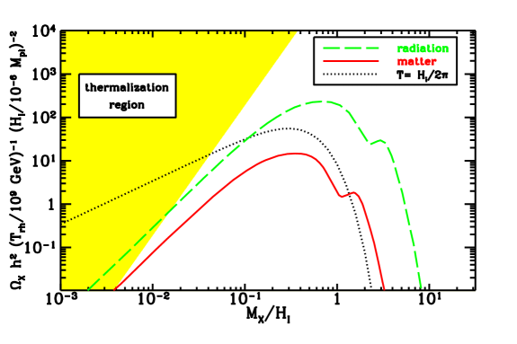
Figure 10: The contribution of gravitationally produced wimpzillas to $\Omega_{X}h^{2}$ as a function of $M_{X}/H_{I}$. The shaded area is where thermalization may occur if the annihilation cross section is its maximum value. Also shown is the contribution assuming that the wimpzilla is present at the end of inflation with a temperature $T=H_{I}/2\pi$.

Start with the canonical quantization of the $X$ field in an action of the form (with metric $ds^{2}=dt^{2}-a^{2}(t)d{\bf x}^{2}=a^{2}(\eta)\left[d\eta^{2}-d{\bf x}^{2}\right]$ where $\eta$ is conformal time)

$$S=\int dt\int d^{3}\!x\,\frac{a^{3}}{2}\left(\dot{X}^{2}-\frac{(\nabla X)^{2}}{a^{2}}-M_{X}^{2}X^{2}-\xi RX^{2}\right)$$ (34)

where $R$ is the Ricci scalar. After transforming to conformal time coordinate, use the mode expansion

$$X({\bf x})=\int\frac{d^{3}\!k}{(2\pi)^{3/2}a(\eta)}\left[a_{k}h_{k}(\eta)e^{i{\bf{k\cdot x}}}+a_{k}^{\dagger}h_{k}^{*}(\eta)e^{-i{\bf{k\cdot x}}}\right],$$ (35)

where because the creation and annihilation operators obey the commutator $[a_{k_{1}},a_{k_{2}}^{\dagger}]=\delta^{(3)}({\bf k}_{1}-{\bf k}_{2})$, the $h_{k}$s obey a normalization condition $h_{k}h_{k}^{{}^{\prime}*}-h_{k}^{\prime}h_{k}^{*}=i$ to satisfy the canonical field commutators (henceforth, all primes on functions of $\eta$ refer to derivatives with respect to $\eta$). The resulting mode equation is

$$h_{k}^{\prime\prime}(\eta)+w_{k}^{2}(\eta)h_{k}(\eta)=0,$$ (36)

where

$$w_{k}^{2}=k^{2}+M_{X}^{2}a^{2}+(6\xi-1)a^{\prime\prime}/a\ .$$ (37)

The parameter $\xi$ is 1/6 for conformal coupling and 0 for minimal coupling. From now on, $\xi=1/6$ for simplicity but without much loss of generality. By a change in variable $\eta\rightarrow k/a$, one can rewrite the differential equation such that it depends only on $H(\eta)$, $H^{\prime}(\eta)/k$, $k/a(\eta)$, and $M_{X}$. Hence, the parameters $H_{I}$ and $a_{I}$ correspond to the Hubble parameter and the scale factor evaluated at an arbitrary conformal time $\eta_{I}$, which can be taken to be the approximate time at which $X$s are produced (i.e., $\eta_{I}$ is the conformal time at the end of inflation).

One may then rewrite Eq. 36 as

$$h_{{\tilde{k}}}^{\prime\prime}({{\tilde{\eta}}})+\left({{\tilde{k}}}^{2}+\frac{M_{X}^{2}}{H_{I}^{2}}\tilde{a}^{2}\right)h_{{\tilde{k}}}({{\tilde{\eta}}})=0\ ,$$ (38)

where ${{\tilde{\eta}}}=\eta a_{I}H_{I}$, $\tilde{a}=a/a_{I}$, and ${{\tilde{k}}}=k/(a_{I}H_{I})$. For simplicity of notation, drop all the tildes. This differential equation can be solved once the boundary conditions are supplied.

The number density of the wimpzillas is found by a Bogoliubov transformation from the vacuum mode solution with the boundary condition at $\eta=\eta_{0}$ (the initial time at which the vacuum of the universe is determined) into the one with the boundary condition at $\eta=\eta_{1}$ (any later time at which the particles are no longer being created). $\eta_{0}$ will be taken to be $-\infty$ while $\eta_{1}$ will be taken to be at $+\infty$. Defining the Bogoliubov transformation as $h_{k}^{\eta_{1}}(\eta)=\alpha_{k}h_{k}^{\eta_{0}}(\eta)+\beta_{k}h_{k}^{*\eta_{0}}(\eta)$ (the superscripts denote where the boundary condition is set), the energy density of produced particles is

$$\rho_{X}(\eta_{1})=M_{X}n_{X}(\eta_{1})=M_{X}H_{I}^{3}\left(\frac{1}{\tilde{a}(\eta_{1})}\right)^{3}\int_{0}^{\infty}\frac{d\tilde{k}}{2\pi^{2}}\tilde{k}^{2}|\beta_{\tilde{k}}|^{2},$$ (39)

where one should note that the number operator is defined at $\eta_{1}$ while the quantum state (approximated to be the vacuum state) defined at $\eta_{0}$ does not change in time in the Heisenberg representation.

As one can see from Eq. 38, the input parameter is $M_{X}/H_{I}$. One must also specify the behavior of $a(\eta)$ near the end of inflation. In Fig. 10 (from [34]), I show the resulting values of $\Omega_{X}h^{2}$ as a function of $M_{X}/H_{I}$ assuming the evolution of the scale factor smoothly interpolates between exponential expansion during inflation and either a matter-dominated universe or radiation-dominated universe. The peak at $M_{X}/H_{I}\sim 1$ is similar to the case presented in Ref. [38]. As expected, for large $M_{X}/H_{I}$, the number density falls off faster than any inverse power of $M_{X}/H_{I}$.

Now most of the action occurs around the transition from inflation to the matter-dominated or radiation-dominated universe. This is shown in Fig. 11. Also from Fig. 11 one can see that most of the particles are created with wavenumber of order $H_{I}$.

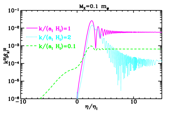
Figure 11: The evolution of the Bogoliubov coefficient with conformal time for several wavenumbers. $\eta=\eta_{I}$ corresponds to the end of the inflationary era.

To conclude, there is a significant mass range ($0.03H_{I}$ to $10H_{I}$, where $H_{I}\sim 10^{13}$GeV) for which wimpzillas will have critical density today regardless of the fine details of the transition out of inflation. Because this production mechanism is inherent in the dynamics between the classical gravitational field and a quantum field, it needs no fine tuning of field couplings or any coupling to the inflaton field. However, only if the particles are stable (or sufficiently long lived) will these particles give contribution of the order of critical density.

3.2.3.b Production During Reheating

Another attractive origin for wimpzillas is during the defrosting phase after inflation. It is important to recall that it is not necessary to convert a significant fraction of the available energy into massive particles; in fact, it must be an infinitesimal amount. I now will discuss how particles of mass much greater than $T_{RH}$ may be created in the correct amount after inflation in reheating [39].

In one extreme is the assumption that the vacuum energy of inflation is immediately converted to radiation resulting in a reheat temperature $T_{RH}$. In this case $\Omega_{X}$ can be calculated by integrating the Boltzmann equation with initial condition $N_{X}=0$ at $T=T_{RH}$. One expects the $X$ density to be suppressed by $\exp(-2M_{X}/T_{RH})$; indeed, one finds $\Omega_{X}\sim 1$ for $M_{X}/T_{RH}\sim 25+0.5\ln(m_{X}^{2}\langle\sigma|v|\rangle)$, in agreement with previous estimates [32] that for $T_{RH}\sim 10^{9}$GeV, the wimpzilla mass would be about $2.5\times 10^{10}$GeV.

It is simple to calculate the wimpzilla abundance in the slow reheating scenario. It will be important to keep in mind that what is commonly called the reheat temperature, $T_{RH}$, is not the maximum temperature obtained after inflation. The maximum temperature is, in fact, much larger than $T_{RH}$. The reheat temperature is best regarded as the temperature below which the universe expands as a radiation-dominated universe, with the scale factor decreasing as $g_{*}^{-1/3}T^{-1}$. In this regard it has a limited meaning [18, 40]. One implication of this is that it is incorrect to assume that the maximum abundance of a massive particle species produced after inflation is suppressed by a factor of $\exp(-M/T_{RH})$.

To estimate wimpzilla production in reheating, consider a model universe with three components: inflaton field energy, $\rho_{\phi}$, radiation energy density, $\rho_{R}$, and wimpzilla energy density, $\rho_{X}$. Assume that the decay rate of the inflaton field energy density is $\Gamma_{\phi}$. Also assume the wimpzilla lifetime is longer than any timescale in the problem (in fact it must be longer than the present age of the universe). Finally, assume that the light degrees of freedom are in local thermodynamic equilibrium.

With the above assumptions, the Boltzmann equations describing the redshift and interchange in the energy density among the different components is [cf. Eq. (3.1.1)]

$$\dot{\rho}_{\phi}+3H\rho_{\phi}+\Gamma_{\phi}\rho_{\phi}=0$$

$$\dot{\rho}_{R}+4H\rho_{R}-\Gamma_{\phi}\rho_{\phi}-\frac{\langle\sigma|v|\rangle}{M_{X}}\left[\rho_{X}^{2}-\left(\rho_{X}^{EQ}\right)^{2}\right]=0$$

$$\dot{\rho}_{X}+3H\rho_{X}+\frac{\langle\sigma|v|\rangle}{M_{X}}\left[\rho_{X}^{2}-\left(\rho_{X}^{EQ}\right)^{2}\right]=0\ ,$$ (40)

where dot denotes time derivative. As already mentioned, $\langle\sigma|v|\rangle$ is the thermal average of the $X$ annihilation cross section times the Møller flux factor. The equilibrium energy density for the $X$ particles, $\rho_{X}^{EQ}$, is determined by the radiation temperature, $T=(30\rho_{R}/\pi^{2}g_{*})^{1/4}$.

It is useful to introduce two dimensionless constants, $\alpha_{\phi}$ and $\alpha_{X}$, defined in terms of $\Gamma_{\phi}$ and $\langle\sigma|v|\rangle$ as

$$\Gamma_{\phi}=\alpha_{\phi}M_{\phi}\qquad\langle\sigma|v|\rangle=\alpha_{X}M_{X}^{-2}\ .$$ (41)

For a reheat temperature much smaller than $M_{\phi}$, $\Gamma_{\phi}$ must be small. From Eq. (23), the reheat temperature in terms of $\alpha_{X}$ and $M_{X}$ is $T_{RH}\simeq\alpha_{\phi}^{1/2}\sqrt{M_{\phi}M_{Pl}}$. For $M_{\phi}=10^{13}$GeV, $\alpha_{\phi}$ must be smaller than of order $10^{-13}$. On the other hand, $\alpha_{X}$ may be as large as of order unity, or it may be small also.

It is also convenient to work with dimensionless quantities that can absorb the effect of the expansion of the universe. This may be accomplished with the definitions

$$\Phi\equiv\rho_{\phi}M_{\phi}^{-1}a^{3}\ ;\quad R\equiv\rho_{R}a^{4}\ ;\quad X\equiv\rho_{X}M_{X}^{-1}a^{3}\ .$$ (42)

It is also convenient to use the scale factor, rather than time, for the independent variable, so one may define a variable $x=aM_{\phi}$. With this choice the system of equations can be written as (prime denotes $d/dx$)

$$\Phi^{\prime} = -c_{1}\ \frac{x}{\sqrt{\Phi x+R}}\ \Phi$$

$$R^{\prime} = c_{1}\ \frac{x^{2}}{\sqrt{\Phi x+R}}\ \Phi\ +c_{2}\ \frac{x^{-1}}{\sqrt{\Phi x+R}}\ \left(X^{2}-X_{EQ}^{2}\right)$$

$$X^{\prime} = -c_{3}\ \frac{x^{-2}}{\sqrt{\Phi x+R}}\ \left(X^{2}-X_{EQ}^{2}\right)\ .$$ (43)

The constants $c_{1}$, $c_{2}$, and $c_{3}$ are given by

$$c_{1}=\sqrt{\frac{3}{8\pi}}\frac{M_{Pl}}{M_{\phi}}\alpha_{\phi}\ \qquad c_{2}=c_{1}\frac{M_{\phi}}{M_{X}}\frac{\alpha_{X}}{\alpha_{\phi}}\ \qquad c_{3}=c_{2}\frac{M_{\phi}}{M_{X}}\ .$$ (44)

$X_{EQ}$ is the equilibrium value of $X$, given in terms of the temperature $T$ as (assuming a single degree of freedom for the $X$ species)

$$X_{EQ}=\frac{M_{X}^{3}}{M_{\phi}^{3}}\left(\frac{1}{2\pi}\right)^{3/2}x^{3}\left(\frac{T}{M_{X}}\right)^{3/2}\exp(-M_{X}/T)\ .$$ (45)

The temperature depends upon $R$ and $g_{*}$, the effective number of degrees of freedom in the radiation:

$$\frac{T}{M_{X}}=\left(\frac{30}{g_{*}\pi^{2}}\right)^{1/4}\frac{M_{\phi}}{M_{X}}\frac{R^{1/4}}{x}\ .$$ (46)

It is straightforward to solve the system of equations in Eq. (3.2.3) with initial conditions at $x=x_{I}$ of $R(x_{I})=X(x_{I})=0$ and $\Phi(x_{I})=\Phi_{I}$. It is convenient to express $\rho_{\phi}(x=x_{I})$ in terms of the expansion rate at $x_{I}$, which leads to

$$\Phi_{I}=\frac{3}{8\pi}\frac{M^{2}_{Pl}}{M_{\phi}^{2}}\frac{H_{I}^{2}}{M_{\phi}^{2}}\ x_{I}^{3}\ .$$ (47)

The numerical value of $x_{I}$ is irrelevant.

Before solving numerically the system of equations, it is useful to consider the early-time solution for $R$. Here, early times means $H\gg\Gamma_{\phi}$, i.e., before a significant fraction of the comoving coherent energy density is converted to radiation. At early times $\Phi\simeq\Phi_{I}$, and $R\simeq X\simeq 0$, so the equation for $R^{\prime}$ becomes $R^{\prime}=c_{1}x^{3/2}\Phi_{I}^{1/2}$. Thus, the early time solution for $R$ is simple to obtain:

$$R\simeq\frac{2}{5}c_{1}\left(x^{5/2}-x_{I}^{5/2}\right)\Phi_{I}^{1/2}\qquad(H\gg\Gamma_{\phi})\ .$$ (48)

Now express $T$ in terms of $R$ to yield the early-time solution for $T$:

$$\frac{T}{M_{\phi}}\simeq\left(\frac{12}{\pi^{2}g_{*}}\right)^{1/4}c_{1}^{1/4}\left(\frac{\Phi_{I}}{x_{I}^{3}}\right)^{1/8}\left[\left(\frac{x}{x_{I}}\right)^{-3/2}-\left(\frac{x}{x_{I}}\right)^{-4}\right]^{1/4}\qquad(H\gg\Gamma_{\phi})\ .$$ (49)

Thus, $T$ has a maximum value of

$$\frac{T_{MAX}}{M_{\phi}} = 0.77\left(\frac{12}{\pi^{2}g_{*}}\right)^{1/4}c_{1}^{1/4}\left(\frac{\Phi_{I}}{x_{I}^{3}}\right)^{1/8}$$ (50)

$$= 0.77\alpha_{\phi}^{1/4}\left(\frac{9}{2\pi^{3}g_{*}}\right)^{1/4}\left(\frac{M_{Pl}^{2}H_{I}}{M_{\phi}^{3}}\right)^{1/4}\ ,$$

which is obtained at $x/x_{I}=(8/3)^{2/5}=1.48$. It is also possible to express $\alpha_{\phi}$ in terms of $T_{RH}$ and obtain

$$\frac{T_{MAX}}{T_{RH}}=0.77\left(\frac{9}{5\pi^{3}g_{*}}\right)^{1/8}\left(\frac{H_{I}M_{Pl}}{T_{RH}^{2}}\right)^{1/4}\ .$$ (51)

For an illustration, in the simplest model of chaotic inflation $H_{I}\sim M_{\phi}$ with $M_{\phi}\simeq 10^{13}$GeV, which leads to $T_{MAX}/T_{RH}\sim 10^{3}(200/g_{*})^{1/8}$ for $T_{RH}=10^{9}$GeV.

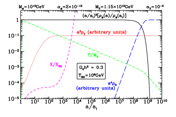
Figure 12: The evolution of energy densities and $T/M_{X}$ as a function of the scale factor. Also shown is $X/X_{EQ}$.

We can see from Eq. (48) that for $x/x_{I}>1$, in the early-time regime $T$ scales as $a^{-3/8}$, which implies that entropy is created in the early-time regime [40]. So if one is producing a massive particle during reheating it is necessary to take into account the fact that the maximum temperature is greater than $T_{RH}$, and that during the early-time evolution, $T\propto a^{-3/8}$.

An example of a numerical evaluation of the complete system in Eq. (3.2.3) is shown in Fig. 12 (from [39]). The model parameters chosen were $M_{\phi}=10^{13}$GeV, $\alpha_{\phi}=2\times 10^{-13}$, $M_{X}=1.15\times 10^{12}$GeV, $\alpha_{X}=10^{-2}$, and $g_{*}=200$. The expansion rate at the beginning of the coherent oscillation period was chosen to be $H_{I}=M_{\phi}$. These parameters result in $T_{RH}=10^{9}$GeV and $\Omega_{X}h^{2}=0.3$.

Figure 12 serves to illustrate several aspects of the problem. Just as expected, the comoving energy density of $\phi$ (i.e., $a^{3}\rho_{\phi}$) remains roughly constant until $\Gamma_{\phi}\simeq H$, which for the chosen model parameters occurs around $a/a_{I}\simeq 5\times 10^{8}$. But of course, that does not mean that the temperature is zero. Notice that the temperature peaks well before “reheating.” The maximum temperature, $T_{MAX}=10^{12}$GeV, is reached at $a/a_{I}$ slightly larger than unity (in fact at $a/a_{I}=1.48$ as expected), while the reheat temperature, $T_{RH}=10^{9}$GeV, occurs much later, around $a/a_{I}\sim 10^{8}$. Note that $T_{MAX}\simeq 10^{3}T_{RH}$ in agreement with Eq. (51).

From the figure it is clear that $X\ll X_{EQ}$ at the epoch of freeze out of the comoving $X$ number density, which occurs around $a/a_{I}\simeq 10^{2}$. The rapid rise of the ratio after freeze out is simply a reflection of the fact that $X$ is constant while $X_{EQ}$ decreases exponentially.

A close examination of the behavior of $T$ shows that after the sharp initial rise of the temperature, the temperature decreases as $a^{-3/8}$ [as follows from Eq. (49)] until $H\simeq\Gamma_{\phi}$, and thereafter $T\propto a^{-1}$ as expected for the radiation-dominated era.

For the choices of $M_{\phi}$, $\alpha_{\phi}$, $g_{*}$, and $\alpha_{X}$ used for the model illustrated in Fig. 12, $\Omega_{X}h^{2}=0.3$ for $M_{X}=1.15\times 10^{12}$GeV, in excellent agreement with the mass predicted by using an analytic estimate for the result [39]

$$\Omega_{X}h^{2}=M_{X}^{2}\langle\sigma|v|\rangle\,\left(\frac{g_{*}}{200}\right)^{-3/2}\,\left(\frac{2000T_{RH}}{M_{X}}\right)^{7}\ .$$ (52)

Here again, the results have also important implications for the conjecture that ultra-high cosmic rays, above the Greisen-Zatsepin-Kuzmin cut-off of the cosmic ray spectrum, may be produced in decays of superheavy long-living particles [31, 32, 33, 41]. In order to produce cosmic rays of energies larger than about $10^{13}$ GeV, the mass of the $X$-particles must be very large, $M_{X}\stackrel{{\scriptstyle>}}{{{}_{\sim}}}10^{13}$ GeV and their lifetime $\tau_{X}$ cannot be smaller than the age of the Universe, $\tau_{X}\stackrel{{\scriptstyle>}}{{{}_{\sim}}}10^{10}$ yr. With the smallest value of the lifetime, the observed flux of ultra-high energy cosmic rays will be reproduced with a rather low density of $X$-particles, $\Omega_{X}\sim 10^{-12}$. It has been suggested that $X$-particles can be produced in the right amount by usual collisions and decay processes taking place during the reheating stage after inflation if the reheat temperature never exceeded $M_{X}$ [41]. Again, assuming naively that that the maximum number density of a massive particle species $X$ produced after inflation is suppressed by a factor of $(M_{X}/T_{RH})^{3/2}\exp(-M_{X}/T_{RH})$ with respect to the photon number density, one concludes that the reheat temperature $T_{RH}$ should be in the range $10^{11}$ to $10^{15}$GeV [32]. This is a rather high value and leads to the gravitino problem in generic supersymmetric models. This is one reason alternative production mechanisms of these superheavy $X$-particles have been proposed [34, 42, 43]. However, our analysis show that the situation is much more promising. Making use of Eq. (52), the right amount of $X$-particles to explain the observed ultra-high energy cosmic rays is produced for

$$\left(\frac{T_{RH}}{10^{10}\>{\rm GeV}}\right)\simeq\left(\frac{g_{*}}{200}\right)^{3/14}\>\left(\frac{M_{X}}{10^{15}\>{\rm GeV}}\right),$$ (53)

where it has been assumed that $\langle\sigma|v|\rangle\sim M_{X}^{-2}$. Therefore, particles as massive as $10^{15}$ GeV may be generated during the reheating stage in abundances large enough to explain the ultra-high energy cosmic rays even if the reheat temperature satisfies the gravitino bound.

3.2.3.c Production During Preheating

Another way to produce wimpzillas after inflation is in a preliminary stage of reheating called “preheating” [21], where nonlinear quantum effects may lead to an extremely effective dissipational dynamics and explosive particle production.

As discussed in Section 3.1.2, particles can be created in a broad parametric resonance with a fraction of the energy stored in the form of coherent inflaton oscillations at the end of inflation released after only a dozen oscillation periods. A crucial observation for our discussion is that particles with mass up to $10^{15}$ GeV may be created during preheating [42, 24, 44], and that their distribution is nonthermal. If these particles are stable, they may be good candidates for wimpzillas [22].

Interestingly enough, what was found [22] is that in the context of a slow-roll inflation with the potential $V(\phi)=m_{\phi}^{2}\phi^{2}/2$ with the inflaton coupling of $g^{2}\phi^{2}X^{2}/2$, the resonance phenomenon is mostly irrelevant to wimpzilla production because too many particles would be produced if the resonance is effective. For the tiny amount of energy conversion needed for wimpzilla production, the coupling $g^{2}$ must be small enough (for a fixed $M_{X}$) such that the motion of the inflaton field at the transition out of the inflationary phase generates just enough nonadiabaticity in the mode frequency to produce wimpzillas. The rest of the oscillations, damped by the expansion of the universe, will not contribute significantly to wimpzilla production as in the resonant case. In other words, the quasi-periodicity necessary for a true resonance phenomenon is not present in the case when only an extremely tiny fraction of the energy density is converted into wimpzillas. Of course, if the energy scales are lowered such that a fair fraction of the energy density can be converted to wimpzillas without overclosing the universe, this argument may not apply.

The main finding of a detailed treatment [22] is that wimpzillas with a mass as large as $10^{3}H_{I}$, where $H_{I}$ is the value of the Hubble expansion rate at the end of inflation, can be produced in sufficient abundance to be cosmologically significant today.

If the wimpzilla is coupled to the inflaton $\phi$ by a term $g^{2}\phi^{2}X^{2}/2$, then the mode equation in Eq. 37 is now changed to

$$\omega_{k}^{2}+k^{2}+\left(M_{X}^{2}+g^{2}\phi^{2}\right)a^{2}\ ,$$ (54)

again taking $\xi=1/6$.

The procedure to calculate the wimpzilla density is the same as in Section 3.2.3. Now, in addition to the parameter $M_{X}/H_{I}$, there is another parameter $gM_{Pl}/H_{I}$. Now in large-field models $H_{I}\sim 10^{13}$GeV, so $M_{Pl}/H_{I}$ might be as large as $10^{6}$. The choice of $g=10^{-3}$ would yield $gM_{Pl}/H_{I}=10^{3}$.

Figure 13: A graph of $\Omega_{X}h^{2}$ versus $M_{X}/H_{I}$ for $gM_{Pl}/H_{I}=10^{6}$. The solid curve is a numerical result, while the dashed and dotted curves are analytic approximations [22].

Fig. 13 (from [22]) shows the dependence of the wimpzilla density upon $M_{X}/H_{I}$ for the particular choice $gM_{Pl}/H_{I}=10^{6}$. This would correspond to $g\sim 1$ in large-field inflation models where $M_{Pl}/H_{I}=10^{6}$, about the largest possible value. Note that $\Omega_{X}\sim 1$ obtains for $M_{X}/H_{I}\approx 10^{3}$. The dashed and dotted curves are two analytic approximations discussed in [22], while the solid curve is the numerical result. The approximations are in very good agreement with the numerical results.

Fig. 14 (from [22]) shows the dependence of the wimpzilla density upon $gM_{Pl}/H_{I}$. For this graph $M_{X}/H_{I}$ was chosen to be unity. This figure illustrates the fact that the dependence of $\Omega_{X}h^{2}$ on $gM_{Pl}/H_{I}$ is not monotonic. For a detailed explanation of this curious effect, see the paper of Chung [22].

Figure 14: An illustration of the nonmonotonic behavior of the particle density produced with the variation of the coupling constant. The value of $M_{X}/H_{I}$ is set to unity [22].

3.2.3.d Production in Bubble Collisions

wimpzillas may also be produced [43] if inflation is completed by a first-order phase transition [45], in which the universe exits from a false-vacuum state by bubble nucleation [46]. When bubbles of true vacuum form, the energy of the false vacuum is entirely transformed into potential energy in the bubble walls. As the bubbles expand, more and more of their energy becomes kinetic as the walls become highly relativistic.

In bubble collisions the walls oscillate through each other [47] and their kinetic energy is dispersed into low-energy scalar waves [47, 48]. We are interested in the potential energy of the walls, $M_{P}=4\pi\eta R^{2}$, where $\eta$ is the energy per unit area of a bubble wall of radius $R$. The bubble walls can be visualized as a coherent state of inflaton particles, so the typical energy $E$ of the products of their decays is simply the inverse thickness of the wall, $E\sim\Delta^{-1}$. If the bubble walls are highly relativistic when they collide, there is the possibility of quantum production of nonthermal particles with mass well above the mass of the inflaton field, up to energy $\Delta^{-1}=\gamma M_{\phi}$, with $\gamma$ the relativistic Lorentz factor.

Suppose for illustration that the wimpzilla is a fermion coupled to the inflaton field by a Yukawa coupling $g\phi\overline{X}{X}$. One can treat $\phi$ (the bubbles or walls) as a classical, external field and the wimpzilla as a quantum field in the presence of this source. The number of wimpzillas created in the collisions from the wall potential energy is $N_{X}\sim f_{X}M_{P}/M_{X}$, where $f_{X}$ parametrizes the fraction of the primary decay products in wimpzillas. The fraction $f_{X}$ will depend in general on the masses and the couplings of a particular theory in question. For the Yukawa coupling $g$, it is $f_{X}\simeq g^{2}{\rm ln}\left(\gamma M_{\phi}/2M_{X}\right)$ [48, 49]. wimpzillas may be produced in bubble collisions out of equilibrium and never attain chemical equilibrium. Even with $T_{RH}$ as low as 100 GeV, the present wimpzilla abundance would be $\Omega_{X}\sim 1$ if $g\sim 10^{-5}\alpha^{1/2}$. Here $\alpha^{-1}\ll 1$ is the fraction of the bubble energy at nucleation in the form of potential energy at the time of collision. This simple analysis indicates that the correct magnitude for the abundance of wimpzillas may be naturally obtained in the process of reheating in theories where inflation is terminated by bubble nucleation.

3.2.4 Wimpzilla Conclusions

In this talk I have pointed out several ways to generate nonthermal dark matter. All of the methods can result in dark matter much more massive than the feeble little weak-scale mass thermal relics. The nonthermal dark matter may be as massive as the GUT scale, truly in the wimpzilla range.

The mass scale of the wimpzillas is determined by the mass scale of inflation, more exactly, the expansion rate of the universe at the end of inflation. For large-field inflation models, that mass scale is of order $10^{13}$GeV. For small-field inflation models, it may be less, perhaps much less.

The mass scale of inflation may one day be measured! In addition to scalar density perturbations, tensor perturbations are produced in inflation. The tensor perturbations are directly proportional to the expansion rate during inflation, so determination of a tensor contribution to cosmic background radiation temperature fluctuations would give the value of the expansion rate of the universe during inflation and set the scale for the mass of the wimpzilla.

Undoubtedly, other methods for wimpzilla production will be developed. But perhaps even with the present scenarios one should start to investigate methods for wimpzilla detection. While wimpy wimps must be color singlets and electrically neutral, wimpzillas may be endowed with color and electric charge. This should open new avenues for detection and exclusion of wimpzillas. The lesson here is that wimpzillas may surprise and be the dark matter, and we may learn that size does matter!

References

- [1] A. H. Guth, Phys. Rev. D23, 347 (1981).
- [2] L. Kofman, A. D. Linde, and A. A. Starobinsky, Phys. Rev. D 56, 3258 (1997).
- [3] For a review, see V. F. Mukhanov, H. A. Feldman, and R. H. Brandenberger. Phys. Rep. 215, 203 (1992).
- [4] S. Dodelson, W. H. Kinney, and E. W. Kolb, Phys. Rev. D56, 3207 (1997) .
- [5] J. E. Lidsey, A. R. Liddle, E. W. Kolb, E. J. Copeland, T. Barreiro and M. Abney, Rev. Mod. Phys. 69, 373 (1997).
- [6] E. J. Copeland, E. W. Kolb, A. R. Liddle and J. E. Lidsey, Phys. Rev. Lett. 71, 219 (1993), Phys. Rev. D 48, 2529 (1993), 49, 1840 (1994); M. S. Turner, Phys. Rev. D 48, 5539 (1993).
- [7] A. R. Liddle and D. H. Lyth, Phys. Rep. 231, 1 (1993).
- [8] I. J. Grivell and A. R. Liddle, Phys. Rev. D 54, 7191 (1996).
- [9] D. S. Salopek and J. R. Bond, Phys. Rev. D 42, 3936 (1990).
- [10] A. R. Liddle and D. H. Lyth, Phys. Lett. B 291, 391 (1992).
- [11] A. R. Liddle, P. Parsons and J. D. Barrow, Phys. Rev. D 50, 7222 (1994).
- [12] E. D. Stewart and D. H. Lyth, Phys. Lett. B 302, 171 (1993).
- [13] G. Jungman, M. Kamionkowski, A. Kosowsky and D. N. Spergel, Phys. Rev. D 54, 1332 (1996); J. R. Bond, G. Efstathiou and M. Tegmark, Mon. Not. R. Astron. Soc. 291, L33 (1997).
- [14] M. Zaldarriaga, D. Spergel and U. Seljak, Astrophys. J. 488, 1 (1997).
- [15] E. J. Copeland, I. J. Grivell and A. R. Liddle, Sussex preprint astro-ph/9712028 (1997).
- [16] E. J. Copeland, I. J. Grivell, E. W. Kolb, and A. R. Liddle, Phys. Rev. D58 043002 (1998) .
- [17] L. Wang, V. F. Mukhanov and P. J. Steinhardt, Phys. Lett. B 414, 18 (1997).
- [18] E. W. Kolb and M. S. Turner, The Early Universe, (Addison-Wesley, Menlo Park, Ca., 1990).
- [19] D. H. Lyth and A. Riotto, hep-ph/9807278.
- [20] J. Ellis, J. Kim and D. V. Nanopoulos, Phys. Lett. B145, 181 (1984); L. M. Krauss, Nucl. Phys. B227, 556 (1983); M. Yu. Khlopov and A. D. Linde, Phys. Lett. 138B, 265 (1984); J. Ellis, D. V. Nanopoulos, and S. Sarkar, Nucl. Phys. B461, 597 (1996).
- [21] L. A. Kofman, A. D. Linde and A. A. Starobinsky, Phys. Rev. Lett. 73, 3195 (1994); S. Yu. Khlebnikov and I. I. Tkachev, Phys. Rev. Lett. 77, 219 (1996); Phys. Lett. B390, 80 (1997); Phys. Rev. Lett. 79, 1607 (1997); Phys. Rev. D 56, 653 (1997); G. W. Anderson, A. Linde and A. Riotto, Phys. Rev. Lett. 77, 3716 (1996); see L. Kofman, The origin of matter in the Universe: reheating after inflation, astro-ph/9605155, UH-IFA-96-28 preprint, 16pp., to appear in Relativistic Astrophysics: A Conference in Honor of Igor Novikov’s 60th Birthday, eds. B. Jones and D. Markovic for a more recent review and a collection of references; see also L. Kofman, A. D. Linde and A. A. Starobinsky, Phys. Rev. D 56, 3258 (1997); J. Traschen and R. Brandenberger, Phys. Rev. D 42, 2491 (1990); Y. Shtanov, J. Traschen, and R. Brandenberger, Phys. Rev. D 51, 5438 (1995).
- [22] D. J. Chung, hep-ph/9809489.
- [23] L. Kofman, A. D. Linde, and A. A. Starobinski, Phys. Rev. Lett. 76, 1011 (1996); I. I. Tkachev, Phys. Lett. B376, 35 (1996).
- [24] E.W. Kolb, A. D. Linde and A. Riotto, Phys. Rev. Lett. 77, 4290 (1996).
- [25] K. Griest and M. Kamionkowski, Phys. Rev. Lett. 64, 615 (1990).
- [26] J. Ellis, J.L. Lopez and D.V. Nanopoulos, Phys. Lett. B247, 257 (1990).
- [27] See, for instance, G. F. Giudice and R. Rattazzi, hep-ph/9801271.
- [28] S. Raby, Phys. Rev. D 56, (1997).
- [29] K. Hamaguchi, Y. Nomura and T. Yanagida, hep-ph/9805346.
- [30] K. Benakli, J. Ellis and D.V. Nanopoulos, hep-ph/9803333.
- [31] D. V. Nanopoulos, ”Proceedings of DARK98,” (1998) L. Baudis and H. Klapdor-Kleingrothaus, eds.
- [32] V. A. Kuzmin and V. A. Rubakov, Phys. Atom. Nucl. 61, 1028 (1998).
- [33] M. Birkel and S. Sarkar, hep-ph/9804285.
- [34] D. J. H. Chung, Edward W. Kolb, and A. Riotto, hep-ph/9802238.
- [35] S. Fulling, Gen. Rel. and Grav. 10, 807 (1979).
- [36] N. D. Birrell and P. C. W. Davies, Quantum Fields in Curved Space (Cambridge University Press, Cambridge, 1982).
- [37] D. M. Chitre and J. B. Hartle, Phys. Rev. D 16, 251 (1977); D. J. Raine and C. P. Winlove, Phys. Rev. D 12, 946 (1975); G. Schaefer and H. Dehnen, Astron. Astrophys. 54, 823 (1977).
- [38] N. D. Birrell and P. C. W. Davies, J. Phys. A:Math. Gen. 13, 2109 (1980).
- [39] D. J. H. Chung, E. W. Kolb, and A. Riotto, hep-ph/9809453.
- [40] R. J. Scherrer and M. S. Turner, Phys. Rev. D31, 681 (1985).
- [41] V. Berezinsky, M. Kachelriess and A. Vilenkin, Phys. Rev. Lett. 79, 4302 (1997).
- [42] V. Kuzmin and I. I. Tkachev, hep-ph/9802304.
- [43] D. J. H. Chung, E. W. Kolb and A. Riotto, hep-ph/9805473.
- [44] E. W. Kolb, A. Riotto and I. I. Tkachev, Phys. Lett. B423, 348 (1998).
- [45] D. La and P. J. Steinhardt, Phys. Rev. Lett. 62, 376 (1989).
- [46] A. H. Guth, Phys. Rev. D 23, 347 (1981).
- [47] S. W. Hawking, I. G. Moss and J. M. Stewart, Phys. Rev. D 26, 2681 (1982).
- [48] R. Watkins and L. Widrow, Nucl. Phys. B374, 446 (1992).
- [49] A. Masiero and A. Riotto, Phys. Lett. B289, 73 (1992).