Parton Distributions, Form Factors and Compton Scattering

Abstract

The soft physics approach to form factors and Compton scattering at moderately large momentum transfer is reviewed. It will be argued that in that approach the Compton cross section is given by the Klein-Nishina cross section multiplied by a factor describing the structure of the proton in terms of two new form factors. These form factors as well as the ordinary electromagnetic form factors represent moments of skewed parton distributions.

QCD provides three valence Fock state contributions to proton form factors, real (RCS) and virtual (VCS) Compton scattering off protons at large momentum transfer: a soft overlap term with an active quark and two spectators, the asymptotically dominant perturbative contribution where by means of the exchange of two hard gluons the quarks are kept collinear with respect to their parent protons and a third contribution that is intermediate between the soft and the perturbative contribution where only one hard gluon is exchanged and one of the three quarks acts as a spectator. Both the soft and the intermediate terms represent power corrections to the perturbative contribution. Higher Fock state contributions are suppressed. The crucial question is what is the relative strengths of the three contributions at experimentally accessible values of momentum transfer, i.e. at $-t$ of the order of 10 GeV²? The pQCD followers assume the dominance of the perturbative contribution and neglect the other two contributions while the soft physics community presumes the dominance of the overlap contribution. Which group is right is not yet fully decided although comparison with the pion case [1] seems to favour a strong overlap contribution.

Let me turn now to the soft physics approach to Compton scattering. For Mandelstam variables, $s$, $t$ and $u$, that are large on a hadronic scale the handbag diagram shown in Fig. 1 describes RCS and VCS. To see this it is of advantage to choose a symmetric frame of reference where the plus and minus light-cone components of $\Delta$ are zero. This implies $t=-\Delta^{2}_{\perp}$ as well as a vanishing skewdness parameter $\zeta=-\Delta^{+}/p^{+}$. To evaluate the skewed parton distributions (SPD) appearing in the handbag diagram and defined in [2], one may use a Fock state decomposition of the proton and sum over all possible spectator configurations. The crucial assumption is then that the soft hadron wave functions are dominated by virtualities in the range $|k_{i}^{2}|\raisebox{-3.0pt}{$\,\stackrel{{\scriptstyle\textstyle<}}{{\sim}}\,$}\Lambda^{2}$, where $\Lambda$ is a hadronic scale of the order of 1 GeV, and by intrinsic transverse parton momenta, $k_{\perp i}$, defined with respect to their parent hadron’s momentum, that satisfy $k_{\perp i}^{2}/x_{i}\raisebox{-3.0pt}{$\,\stackrel{{\scriptstyle\textstyle<}}{{\sim}}\,$}\Lambda^{2}$. Under this assumption factorisation of the Compton amplitude in a hard photon-parton subprocess amplitude and a soft proton matrix element is achieved [3]. This proton matrix element is described by new form factors specific to Compton scattering.

Figure 1: The handbag diagram for Compton scattering. The momenta of the incoming and outgoing protons (photons) are denoted by $p$ ($q$) and $p^{\prime}=p+\Delta$ ($q^{\prime}=q-\Delta$), respectively.

As a consequence of this result the Compton amplitudes conserving the proton helicity are given by

$${\cal M}_{\mu^{\prime}+,\,\mu+}\,=\,\;2\pi\alpha_{\rm em}\left[{\cal H}_{\mu^{\prime}+,\,\mu+}\,(R_{V}+R_{A})\,+\,{\cal H}_{\mu^{\prime}-,\,\mu-}\,(R_{V}-R_{A})\right]\,.$$ (1)

Proton helicity flip is neglected. $\mu$ and $\mu^{\prime}$ are the helicities of the incoming and outgoing photon in the photon-proton cms, respectively. The photon-quark subprocess amplitudes, ${\cal H}$, are calculated for massless quarks in lowest order QED. The form factors in Eq. (1), $R_{V}$ and $R_{A}$, represent $1/x$-moments of SPDs at zero skewedness parameter. $R_{V}$ is defined by

$$\sum_{a}e_{a}^{2}\,\int_{0}^{1}\,\frac{{\rm d}x}{x}\,p^{+}\int{{\rm d}z^{-}\over 2\pi}\,e^{i\,xp^{+}z^{-}}\langle p^{\prime}|\,\overline{\psi}{}_{a}(0)\,\gamma^{+}\,\psi_{a}(z^{-})-\overline{\psi}{}_{a}(z^{-})\,\gamma^{+}\,\psi_{a}(0)\,|p\rangle$$

$$=R_{V}(t)\,\bar{u}(p^{\prime})\,\gamma^{+}u(p)\,+R_{T}(t)\,\frac{i}{2m}\bar{u}(p^{\prime})\sigma^{+\rho}\Delta_{\rho}u(p)\,,\hskip 56.9055pt$$ (2)

where the sum runs over quark flavours $a$ ($u$, $d$, …), $e_{a}$ being the electric charge of quark $a$ in units of the positron charge. $R_{T}$ being related to proton helicity flips, is neglected in (1). There is an analogous equation for the axial vector proton matrix element, which defines the form factor $R_{A}$. Due to time reversal invariance the form factors $R_{V}$, $R_{A}$ etc. are real functions.

As shown in [3] form factors can be represented as generalized Drell-Yan light-cone wave function overlaps. Assuming a plausible Gaussian $k_{\perp i}$-dependence of the soft Fock state wave functions, one can explicitly carry out the momentum integrations in the Drell-Yan formula. For simplicity one may further assume a common transverse size parameter, $\hat{a}$, for all Fock states. This immediately allows one to sum over them, without specifying the $x_{i}$-dependence of the wave functions. One then arrives at [3, 4]

$$F_{1}(t) = \sum_{a}\,e_{a}\,\int{\rm d}x\,\exp{\left[\frac{1}{2}\hat{a}^{2}t\frac{1-x}{x}\right]}\,\{q_{a}(x)-\bar{q}_{a}(x)\}\,,$$

$$R_{V}(t) = \sum_{a}\,e_{a}^{2}\,\int\frac{{\rm d}x}{x}\,\exp{\left[\frac{1}{2}\hat{a}^{2}t\frac{1-x}{x}\right]}\,\{q_{a}(x)+\bar{q}_{a}(x)\}\,,$$ (3)

and the analogue for $R_{A}$ with $q_{a}+\bar{q}_{a}$ replaced by $\Delta q_{a}+\Delta\bar{q}_{a}$. $q_{a}$ and $\Delta q_{a}$ are the usual unpolarized and polarized parton distributions, respectively. The result for $F_{1}$ has been derived in Ref. [5] long time ago.

The only parameter appearing in (3) is the effective transverse size parameter $\hat{a}$; it is known to be about 1 GeV^-1 with an uncertainty of about 20$\%$. Thus, this parameter only allows some fine tuning of the results for the form factors. Evaluating, for instance, the form factors from the parton distributions derived by Glück et al. (GRV) [6] with $\hat{a}=1\,GeV^{-1}$, one already finds good results. Improvements are obtained by treating the lowest three Fock states explicitly with specified $x$-dependencies [3]. Results for $t^{2}F_{1}$ and $t^{2}R_{V}$ obtained that way are displayed in Fig. 2. Both the scaled form factors, as well as $t^{2}R_{A}$, exhibit broad maxima and, hence, mimic dimensional counting rule behaviour in the $t$-range from about 5 to 15 GeV². The position, $t_{0}$, of the maximum of $t^{2}F_{i}$, where $F_{i}$ is one of the soft form factors, is determined by the solution of the implicit equation

$$-t=4\hat{a}^{-2}\,\left\langle{\frac{1-x}{x}}\right\rangle^{-1}_{F_{i},t}\,.$$ (4)

The mean value $\langle\frac{1-x}{x}\rangle$ comes out around $0.5$ at $t=t_{0}$, hence, $t_{0}\simeq 8\hat{a}^{2}$. Since both sides of Eq. (4) increase with $-t$ the maximum of the scaled form factor, $F_{i}$, is quite broad. For very large momentum transfer the form factors turn gradually into the soft physics asymptotics $\sim 1/t^{4}$. This is the region where the perturbative contribution ($\sim 1/t^{2}$) takes the lead.

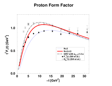
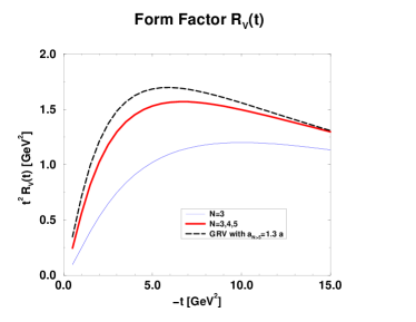
Figure 2: The Dirac (left) and the vector Compton (right) form factor of the proton as predicted by the soft physics approach [3, 7]. Data are taken from [8]. The data on the magnetic form factor, $G_{M}$, are shown in order to demonstrate the size of spin-flip effects.

The amplitude (1) leads to the RCS cross section

$$\frac{{\rm d}\sigma}{{\rm d}t}\,=\,\frac{{\rm d}\hat{\sigma}}{{\rm d}t}\left[\,\frac{1}{2}(R_{V}^{2}(t)+R_{A}^{2}(t))-\,\frac{us}{s^{2}+u^{2}}\,(R_{V}^{2}(t)-R_{A}^{2}(t))\,\right]\,.$$ (5)

It is given by the Klein-Nishina cross section

$$\frac{{\rm d}\hat{\sigma}}{{\rm d}t}\,=\,\frac{2\pi\alpha_{\rm em}^{2}}{s^{2}}\;\frac{s^{2}+u^{2}}{-us}$$ (6)

multiplied by a factor that describes the structure of the proton in terms of two form factors. Evidently, if the form factors scale as $1/t^{2}$, the Compton cross section would scale as $s^{-6}$ at fixed cm scattering angle $\theta$. In view of the above discussion (see also Fig. 2) one therefore infers that approximate dimensional counting rule behaviour holds in a limited range of energy.

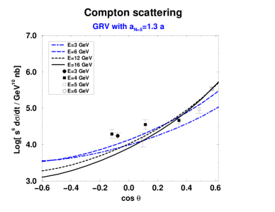
Figure 3: The Compton cross section, scaled by $s^{6}$, (left) and the initial state helicity correlation $A_{\rm LL}$ (right) as predicted by the soft physics approach [3]. Data taken from [9].

The magnitude of the Compton cross section is quite well predicted as is revealed by comparison with the admittedly old data [9] measured at rather low values of $s$, $-t$ and $-u$ (see Fig. 3).

The soft physics approach also predicts characteristic spin dependencies of the Compton process [10]. Of particular interest is the initial state helicity correlation

$$A_{\rm LL}\,\frac{{\rm d}\sigma}{{\rm d}t}=\frac{2\pi\alpha_{\rm em}^{2}}{s^{2}}\;R_{V}(t)R_{A}(t)\left(\frac{u}{s}-\frac{s}{u}\right)\,.$$ (7)

Approximately, $A_{\rm LL}$ is given by the corresponding subprocess helicity correlation $\hat{A}_{\rm LL}=(s^{2}-u^{2})/(s^{2}+u^{2})$ multiplied by the dilution factor $R_{A}(t)/R_{V}(t)$. Thus, measurements of both the cross section and the initial state helicity correlation allows one to isolate the two form factors $R_{V}$ and $R_{A}$ experimentally [11]. In Fig. 3 predictions for $A_{\rm LL}$ are shown.

Other polarization observables as well as the VCS contribution to the unpolarized $ep\to ep\gamma$ cross section have also been predicted in [10]. In addition to VCS the full $ep\to ep\gamma$ cross section receives substantial contributions from the Bethe-Heitler process, in which the final state photon is radiated by the electron. Dominance of the VCS contribution requires high energies, small values of $|\cos{\theta}|$ and an out-of-plane experiment, i.e. an azimuthal angle larger than about $60^{\circ}$. For VCS there are characteristic differences to the diquark model [12], the only other available study of VCS. In the soft physics approach all amplitudes are real (if the photon-parton subprocess is calculated to lowest order perturbation theory [3, 10]) while in the diquark model there are perturbatively generated phase differences among the VCS amplitudes. So, for instance, the beam asymmetry for $ep\to ep\gamma$

$$A_{\rm L}=\frac{{\rm d}\sigma(+)-{\rm d}\sigma(-)}{{\rm d}\sigma(+)+{\rm d}\sigma(-)}\,,$$ (8)

where the labels $+$ and $-$ denote the lepton beam helicity, is zero in the soft physics approachin contrast to the diquark model where a sizeable beam asymmetry is predicted.

In summary, the soft physics approach leads to a simple representation of form factors and to detailed predictions for RCS and VCS. These predictions exhibit interesting features and characteristic spin dependences with marked differences to other approaches. Dimensional counting rule behaviour for form factors, Compton scattering and perhaps for other exlusive observables is mimicked in a limited range of momentum transfer. This tells us that it is premature to infer the dominance of perturbative physics from the observed scaling behaviour, see also [13]. The soft contributions although formally representing power corrections to the asymptotically leading perturbative ones, seem to dominate form factors and Compton scattering for momentum transfers around 10  GeV² (see the discussion in [7, 14]). However, a severe confrontation of this approach with accurate large momentum transfer data on RCS and VCS is still pending.

References

- [1] R. Jakob and P. Kroll, Phys. Lett. B315, 463 (1993), Erratum ibid. B319, 545 (1993); P. Kroll and M. Raulfs, Phys. Lett. B387, 848 (1996); V. Braun and I. Halperin, Phys. Lett. B328, 457 (1994); L.S. Kisslinger and S.W. Wang, Nucl. Phys. B399, 63 (1993).
- [2] D. Müller et al., Fortschr. Physik 42, 101 (1994), hep-ph/9812448; X. Ji, Phys. Rev. Lett. 78, 610 (1997); Phys. Rev. D55, 7114 (1997); A.V. Radyushkin, Phys. Rev. D56, 5524 (1997).
- [3] M. Diehl, T. Feldmann, R. Jakob and P. Kroll, Eur. Phys. J. C8, 409 (1999).
- [4] A.V. Radyushkin, Phys. Rev. D58, 114008 (1998).
- [5] V. Barone et al., Z. Phys. C5, 541 (1993).
- [6] M. Glück, E. Reya and A. Vogt, Z. Phys. C67, 433 (1995); Eur. Phys. J. C5, 461 (1998); M. Glück, E. Reya, M. Stratmann and W. Vogelsang, Phys. Rev. D53, 4775 (1996).
- [7] J. Bolz and P. Kroll, Z. Phys. A356, 327 (1996).
- [8] A.F. Sill et al., Phys. Rev. D48, 29 (1993).
- [9] M.A. Shupe et al., Phys. Rev. D19, 1921 (1979).
- [10] M. Diehl, T. Feldmann, R. Jakob and P. Kroll, Phys. Lett. B460, 204 (1999).
- [11] A.M. Nathan, hep-ph/9908522.
- [12] P. Kroll, M. Schürmann and P.A.M. Guichon, Nucl. Phys. A598, 435 (1996).
- [13] B. Kundu, P. Jain, J.P. Ralston and J. Samuelsson, hep-ph/9909239.
- [14] J. Bolz, R. Jakob, P. Kroll, M. Bergmann and N.G. Stefanis, Z. Phys. C66, 267 (1995).