Techniques for QCD calculations by numerical integration

Abstract

Calculations of observables in quantum chromodynamics are typically performed using a method that combines numerical integrations over the momenta of final state particles with analytical integrations over the momenta of virtual particles. I describe the most important steps of a method for performing all of the integrations numerically.

I Introduction

This paper concerns a method, which was introduced in [1], for performing perturbative calculations in quantum chromodynamics (QCD) and other quantum field theories. The method is intended for calculations of quantities in which one measures something about the hadronic final state produced in a collision and in which the observable is infrared safe – that is, insensitive to long-distance effects. Examples include jet cross sections in hadron-hadron and lepton-hadron scattering and in $e^{+}e^{-}\to{\it hadrons}$. There have been many calculations of this kind carried out at next-to-leading order in perturbation theory. These calculations are based on a method introduced by Ellis, Ross, and Terrano [2] in the context of $e^{+}e^{-}\to{\it hadrons}$. Stated in the simplest terms, the Ellis-Ross-Terrano method is to do some integrations over momenta $\vec{\ell}_{i}$ analytically, others numerically. In the method discussed here, one does all of these integrations numerically. Evidently, if one performs all of the integrations numerically, one gains flexibility to quite easily modify the integrand. There may be other advantages, as well as some disadvantages, to the numerical integration method compared to the numerical/analytical method.

In this paper, I address only the process $e^{+}e^{-}\to{\it hadrons}$. I discuss three-jet-like infrared safe observables at next-to-leading order, that is order $\alpha_{s}^{2}$. Examples of such observables include the thrust distribution and the fraction of events that have three jets.

The main techniques of the numerical integration method for $e^{+}e^{-}\to{\it hadrons}$ were presented briefly in [1]. The principle purpose of this paper is to explain in detail some of the most important of these techniques. In the numerical/analytical method, one has to work hard to implement the cancellation of “collinear” and “soft” divergences that occur in the integrations. In the numerical method, as we will see, this cancellation happens automatically. On the other hand, in the completely numerical method one has the complication of having to deform some of the integration contours into the complex plane. We will see how to do this deformation. In both the numerical/analytical method and the completely numerical method, one must arrange that the density of integration points is singular near a soft gluon singularity of the integrand (even after cancellations). However, the precise behavior of the densities needed in the two cases is different. We will see what is needed in the numerical method.

These techniques are presented in Secs. II-VI. They are illustrated in Sec. VII with a numerical example. Although a full understanding of the example requires the preceding sections, the reader may want to look briefly at Sec. VII before starting on Secs. II-VI. A brief summary of techniques not presented in detail in this paper is given in Sec. VIII.

In [1], I presented results from a concrete implementation of the numerical method in computer code. Since then, one logical error in the code has been discovered and fixed and the performance of the program has been improved. Results from the improved code [3] are presented in Sec. IX.

Let us begin with a precise statement of the problem. We consider an observable such as a particular moment of the thrust distribution. The observable can be expanded in powers of $\alpha_{s}/\pi$,

$$\sigma=\sum_{n}\sigma^{[n]},\hskip 28.45274pt\sigma^{[n]}\propto\left(\alpha_{s}/\pi\right)^{n}\,.$$ (1)

The order $\alpha_{s}^{2}$ contribution has the form

$$\sigma^{[2]} = {1\over 2!}\int d\vec{k}_{1}d\vec{k}_{2}\ {d\sigma^{[2]}_{2}\over d\vec{k}_{1}d\vec{k}_{2}}\ {\cal S}_{2}(\vec{k}_{1},\vec{k}_{2})$$ (4)

$$+{1\over 3!}\int d\vec{k}_{1}d\vec{k}_{2}d\vec{k}_{3}\ {d\sigma^{[2]}_{3}\over d\vec{k}_{1}d\vec{k}_{2}d\vec{k}_{3}}\ {\cal S}_{3}(\vec{k}_{1},\vec{k}_{2},\vec{k}_{3})$$

$$+{1\over 4!}\int d\vec{k}_{1}d\vec{k}_{2}d\vec{k}_{3}d\vec{k}_{4}\ {d\sigma^{[2]}_{4}\over d\vec{k}_{1}d\vec{k}_{2}d\vec{k}_{3}d\vec{k}_{4}}\ {\cal S}_{4}(\vec{k}_{1},\vec{k}_{2},\vec{k}_{3},\vec{k}_{4}).$$

Here the $d\sigma^{[2]}_{n}$ are the order $\alpha_{s}^{2}$ contributions to the parton level cross section, calculated with zero quark masses. Each contains momentum and energy conserving delta functions. The $d\sigma^{[2]}_{n}$ include ultraviolet renormalization in the $\overline{\rm MS}$ scheme. The functions $\cal S$ describe the measurable quantity to be calculated. We wish to calculate a “three-jet-like” quantity. That is, ${\cal S}_{2}=0$. The normalization is such that ${\cal S}_{n}=1$ for $n=2,3,4$ would give the order $\alpha_{s}^{2}$ perturbative contribution the the total cross section. There are, of course, infrared divergences associated with Eq. (4). For now, we may simply suppose that an infrared cutoff has been supplied.

The measurement, as specified by the functions ${\cal S}_{n}$, is to be infrared safe, as described in Ref. [4]: the ${\cal S}_{n}$ are smooth functions of the parton momenta and

$${\cal S}_{n+1}(\vec{k}_{1},\dots,\lambda\vec{k}_{n},(1-\lambda)\vec{k}_{n})={\cal S}_{n}(\vec{k}_{1},\dots,\vec{k}_{n})$$ (5)

for $0\leq\lambda<1$. That is, collinear splittings and soft particles do not affect the measurement.

It is convenient to calculate a quantity that is dimensionless. Let the functions ${\cal S}_{n}$ be dimensionless and eliminate the remaining dimensionality in the problem by dividing by $\sigma_{0}$, the total $e^{+}e^{-}$ cross section at the Born level. Let us also remove the factor of $(\alpha_{s}/\pi)^{2}$. Thus, we calculate

$${\cal I}={\sigma^{[2]}\over\sigma_{0}\ (\alpha_{s}/\pi)^{2}}.$$ (6)

Our problem is thus to calculate ${\cal I}$. Let us now see how to set up this problem in a convenient form. We note that ${\cal I}$ is a function of the c.m. energy $\sqrt{s}$ and the $\overline{\rm MS}$ renormalization scale $\mu$. We will choose $\mu$ to be proportional to $\sqrt{s}$: $\mu=A_{UV}\sqrt{s}$. Then ${\cal I}$ depends on $A$. But, because it is dimensionless, it is independent of $\sqrt{s}$. This allows us to write

$${\cal I}=\int_{0}^{\infty}d\sqrt{s}\ h(\sqrt{s})\ {\cal I}(A_{UV},\sqrt{s}),$$ (7)

where $h$ is any function with

$$\int_{0}^{\infty}d\sqrt{s}\ h(\sqrt{s})=1.$$ (8)

FIG. 1.: Two cuts of one of the Feynman diagrams that contribute to $e^{+}e^{-}\to{\it hadrons}$.

The quantity $\cal I$ can be expressed in terms of cut Feynman diagrams, as in Fig. 1. The dots where the parton lines cross the cut represent the function ${\cal S}_{n}(\vec{k}_{1},\dots,\vec{k}_{n})$. Each diagram is a three loop diagram, so we have integrations over loop momenta $\ell_{1}^{\mu}$, $\ell_{2}^{\mu}$ and $\ell_{3}^{\mu}$. We first perform the energy integrations. For the graphs in which four parton lines cross the cut, there are four mass-shell delta functions $\delta(k_{J}^{2})$. These delta functions eliminate the three energy integrals over $\ell_{1}^{0}$, $\ell_{2}^{0}$, and $\ell_{3}^{0}$ as well as the integral (8) over $\sqrt{s}$. For the graphs in which three parton lines cross the cut, we can eliminate the integration over $\sqrt{s}$ and two of the $\ell_{J}^{0}$ integrals. One integral over the energy $E$ in the virtual loop remains. We perform this integration by closing the integration contour in the lower half $E$ plane. This gives a sum of terms obtained from the original integrand by some algebraic substitutions, as we will see in the following sections. Having performed the energy integrations, we are left with an integral of the form

$${\cal I}=\int d\vec{\ell}_{1}\,d\vec{\ell}_{2}\,d\vec{\ell}_{3}\ \sum_{G}\,\sum_{C}\,g(G,C;\vec{\ell}_{1},\vec{\ell}_{2},\vec{\ell}_{3}).$$ (9)

Here there is a sum over graphs $G$ (of which one is shown in Fig. 1) and there is a sum over the possible cuts of a given graph.

The problem of calculating ${\cal I}$ is now set up in a convenient form for calculation. If we were using the Ellis-Ross-Terrano method, we would calculate some of the integrals in Eq. (9) numerically and some analytically. In the method described here, we first perform certain contour deformations, then calculate all of the integrals by Monte Carlo numerical integration. In the following sections, we will learn the main techniques for performing the integrations in Eq. (9). We will do this by studying a simple model problem that will enable us to see the essential features of the numerical method with as few extraneous difficulties as possible.

II A simplified model

In the following sections, we consider a simplified model in which all complications that are not needed for a first understanding of the numerical method are stripped away. The model is represented by the graph shown in Fig. 2. There are contributions from all of the two and three parton cuts of this diagram, as shown in Fig. 3. Since QCD numerator functions do not play a major role, we consider this graph in $\phi^{3}$ theory. Thus, also, we can avoid the complications of ultraviolet renormalization. We consider the incoming momentum $\vec{q}$ to be fixed and nonzero. We calculate the integral of the graph over the incoming energy $q^{0}$. This is analogous to the technical trick of integrating over $\sqrt{s}$ in the full three loop QCD calculation (see Sec. I) and serves to provide three energy integrations to perform against three mass-shell delta functions for the three-parton cuts.

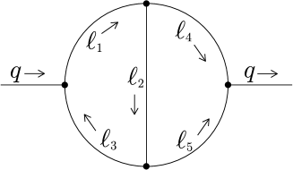
FIG. 2.: Diagram for a simple calculation. All two and three parton cuts of this diagram in $\phi^{3}$ theory are used, with a measurement function that gives the average transverse energy in the final state.

We need a nontrivial measurement function $\cal S$. As an example, we choose to measure the transverse energy in the final state normalized to the total energy:

$${\cal S}_{2}(\vec{k}_{1},\vec{k}_{2}) = (|\vec{k}_{T,1}|+|\vec{k}_{T,2}|)/(|\vec{k}_{1}|+|\vec{k}_{2}|)$$ (10)

$${\cal S}_{3}(\vec{k}_{1},\vec{k}_{2},\vec{k}_{3}) = (|\vec{k}_{T,1}|+|\vec{k}_{T,2}|+|\vec{k}_{T,3}|)/(|\vec{k}_{1}|+|\vec{k}_{2}|+|\vec{k}_{3}|),$$ (11)

where $\vec{k}_{T,j}$ is the part of the momentum $\vec{k}_{j}$ of the $j$th final state particle that is orthogonal to $\vec{q}$.

There are two loops in our diagram. We choose the independent loop momenta to be $\ell_{2}^{\mu}$ and $\ell_{4}^{\mu}$. The other momenta are understood to be expressed in terms of $\ell_{2}^{\mu}$, $\ell_{4}^{\mu}$, and $q^{\mu}$.

FIG. 3.: The two and three parton cuts of the simple $\phi^{3}$ diagram.

Thus the example integral that we seek to calculate is

$${\cal I}={g^{4}\over 2}\int\!{dq^{0}\over 2\pi}\int\!{d^{4}\ell_{2}\over(2\pi)^{4}}\int\!{d^{4}\ell_{4}\over(2\pi)^{4}}\ {\cal W}.$$ (12)

Here $g$ is the coupling, $1/2$ is the statistical factor for this graph, and the integrand ${\cal W}$ consists of four parts, one for each of the cuts in Fig. 3:

$${\cal W}={\cal W}_{a}+{\cal W}_{b}+{\cal W}_{c}+{\cal W}_{d},$$ (13)

where

$${\cal W}_{a} = {i}{\cal S}_{2}(\vec{\ell}_{4},\vec{\ell}_{5})\,{1\over\ell_{1}^{2}+i\epsilon}\,{1\over\ell_{2}^{2}+i\epsilon}\,{1\over\ell_{3}^{2}+i\epsilon}\,(2\pi)\Delta(\ell_{4})\,(2\pi)\Delta(\ell_{5}),$$ (14)

$${\cal W}_{b} = {-i}{\cal S}_{2}(\vec{\ell}_{1},-\vec{\ell}_{3})\,(2\pi)\Delta(\ell_{1})\,{1\over\ell_{2}^{2}-i\epsilon}\,(2\pi)\Delta(-\ell_{3})\,{1\over\ell_{4}^{2}-i\epsilon}\,{1\over\ell_{5}^{2}-i\epsilon},$$ (15)

$${\cal W}_{c} = {\cal S}_{3}(\vec{\ell}_{1},-\vec{\ell}_{2},\vec{\ell}_{5})\,(2\pi)\Delta(\ell_{1})\,(2\pi)\Delta(-\ell_{2})\,{1\over\ell_{3}^{2}}{1\over\ell_{4}^{2}}\,(2\pi)\Delta(\ell_{5}),$$ (16)

$${\cal W}_{d} = {\cal S}_{3}(\vec{\ell}_{4},\vec{\ell}_{2},-\vec{\ell}_{3})\,{1\over\ell_{1}^{2}}\,(2\pi)\Delta(\ell_{2})\,(2\pi)\Delta(-\ell_{3})\,(2\pi)\Delta(\ell_{4})\,{1\over\ell_{5}^{2}}.$$ (17)

Here we have used the notation

$$\Delta(k)=\delta(k^{2})\,\theta(k^{0}).$$ (18)

III The integration over energies

We begin by performing the integrals over the energies in Eq. (12). In the case of three partons in the final state, the three delta functions eliminate the three integrations. In the case of two partons in the final state, the two delta functions eliminate two of the energy integrations. This leaves one integration over the energy that circulates around the virtual loop. There are three poles in the upper half plane and three in the lower half plane. Closing the contour in one half plane or the other gives three contributions. Each of these contributions corresponds to putting one of the particles in the loop on shell. Thus altogether there are eight contributions to ${\cal I}$, as indicated in Fig. 4. We write ${\cal I}$ as

$${\cal I}={g^{4}\over 2(2\pi)^{6}}\int\!d\vec{\ell}_{4}\ \int\!d\vec{\ell}_{2}\ {\cal G},$$ (19)

where the integrand ${\cal G}$ has eight parts:

$${\cal G}={\cal G}_{a1}+{\cal G}_{a2}+{\cal G}_{a3}+{\cal G}_{b5}+{\cal G}_{b2}+{\cal G}_{b4}+{\cal G}_{c}+{\cal G}_{d}.$$ (20)

The contributions to ${\cal G}$ are

$${\cal G}_{a1} = {\cal S}_{2}(\vec{\ell}_{4},\vec{\ell}_{5})\,{1\over 2|\vec{\ell}_{1}|}\,{1\over(|\vec{\ell}_{1}|-|\vec{\ell}_{4}|)^{2}-\vec{\ell}_{2}^{\,2}+i\epsilon}\,{1\over(|\vec{\ell}_{1}|-|\vec{\ell}_{4}|-|\vec{\ell}_{5}|)^{2}-\vec{\ell}_{3}^{\,2}+i\epsilon}\,{1\over 2|\vec{\ell}_{4}|}\,{1\over 2|\vec{\ell}_{5}|},$$ (21)

$${\cal G}_{a2} = {\cal S}_{2}(\vec{\ell}_{4},\vec{\ell}_{5})\,{1\over(|\vec{\ell}_{2}|+|\vec{\ell}_{4}|)^{2}-\vec{\ell}_{1}^{\,2}+i\epsilon}\,{1\over 2|\vec{\ell}_{2}|}\,{1\over(|\vec{\ell}_{2}|-|\vec{\ell}_{5}|)^{2}-\vec{\ell}_{3}^{\,2}+i\epsilon}\,{1\over 2|\vec{\ell}_{4}|}\,{1\over 2|\vec{\ell}_{5}|},$$ (22)

$${\cal G}_{a3} = {\cal S}_{2}(\vec{\ell}_{4},\vec{\ell}_{5})\,{1\over(|\vec{\ell}_{3}|+|\vec{\ell}_{4}|+|\vec{\ell}_{5}|)^{2}-\vec{\ell}_{1}^{\,2}+i\epsilon}\,{1\over(|\vec{\ell}_{3}|+|\vec{\ell}_{5}|)^{2}-\vec{\ell}_{2}^{\,2}+i\epsilon}\,{1\over 2|\vec{\ell}_{3}|}\,{1\over 2|\vec{\ell}_{4}|}\,{1\over 2|\vec{\ell}_{5}|},$$ (23)

$${\cal G}_{b5} = {\cal S}_{2}(\vec{\ell}_{1},-\vec{\ell}_{3})\,{1\over 2|\vec{\ell}_{1}|}\,{1\over(|\vec{\ell}_{3}|+|\vec{\ell}_{5}|)^{2}-\vec{\ell}_{2}^{\,2}-i\epsilon}\,{1\over 2|\vec{\ell}_{3}|}\,{1\over(|\vec{\ell}_{1}|+|\vec{\ell}_{3}|+|\vec{\ell}_{5}|)^{2}-\vec{\ell}_{4}^{\,2}-i\epsilon}\,{1\over 2|\vec{\ell}_{5}|},$$ (24)

$${\cal G}_{b2} = {\cal S}_{2}(\vec{\ell}_{1},-\vec{\ell}_{3})\,{1\over 2|\vec{\ell}_{1}|}\,{1\over 2|\vec{\ell}_{2}|}\,{1\over 2|\vec{\ell}_{3}|}\,{1\over(|\vec{\ell}_{1}|+|\vec{\ell}_{2}|)^{2}-\vec{\ell}_{4}^{\,2}-i\epsilon}\,{1\over(|\vec{\ell}_{3}|-|\vec{\ell}_{2}|)^{2}-\vec{\ell}_{5}^{\,2}-i\epsilon},$$ (25)

$${\cal G}_{b4} = {\cal S}_{2}(\vec{\ell}_{1},-\vec{\ell}_{3})\,{1\over 2|\vec{\ell}_{1}|}\,{1\over(|\vec{\ell}_{1}|-|\vec{\ell}_{4}|)^{2}-\vec{\ell}_{2}^{\,2}-i\epsilon}\,{1\over 2|\vec{\ell}_{3}|}\,{1\over 2|\vec{\ell}_{4}|}\,{1\over(|\vec{\ell}_{1}|+|\vec{\ell}_{3}|-|\vec{\ell}_{4}|)^{2}-\vec{\ell}_{5}^{\,2}-i\epsilon},$$ (26)

$${\cal G}_{c} = {\cal S}_{3}(\vec{\ell}_{1},-\vec{\ell}_{2},\vec{\ell}_{5})\,{1\over 2|\vec{\ell}_{1}|}\,{1\over 2|\vec{\ell}_{2}|}\,{1\over(|\vec{\ell}_{2}|+|\vec{\ell}_{5}|)^{2}-\vec{\ell}_{3}^{\,2}}\,{1\over(|\vec{\ell}_{1}|+|\vec{\ell}_{2}|)^{2}-\vec{\ell}_{4}^{\,2}}\,{1\over 2|\vec{\ell}_{5}|},$$ (27)

$${\cal G}_{d} = {\cal S}_{3}(\vec{\ell}_{4},\vec{\ell}_{2},-\vec{\ell}_{3})\,{1\over(|\vec{\ell}_{2}|+|\vec{\ell}_{4}|)^{2}-\vec{\ell}_{1}^{\,2}}\,{1\over 2|\vec{\ell}_{2}|}\,{1\over 2|\vec{\ell}_{3}|}\,{1\over 2|\vec{\ell}_{4}|}\,{1\over(|\vec{\ell}_{2}|+|\vec{\ell}_{3}|)^{2}-\vec{\ell}_{5}^{\,2}}.$$ (28)

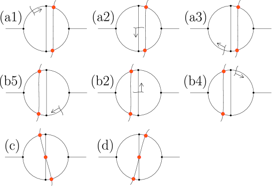
FIG. 4.: The eight contributions to the sample diagram after performing the energy integrations. The line through a propagator in a loop indicates that this propagator is put on shell, with positive energy flowing in the direction of the arrow. The direction for positive energy flow around the loop depends on whether the contour over loop energy is closed in the upper or the lower half plane.

So far, the operations that we have performed have been purely algebraic. They are evidently of a sort that can be easily implemented in a computer program in an automatic fashion. We are left with an integral over the loop momenta $\vec{\ell}_{2}$ and $\vec{\ell}_{4}$. We seek to perform this integration numerically. However, the integrand $\cal G$ has singularities, so it is not completely self-evident how to proceed. It is to this question that we now turn.

IV Cancellation of singularities

In this section, we discuss the cancellation of singularities in a numerical calculation of the integral in Eq. (19).

Let us concentrate to begin with on the cut shown in Fig. 3(a). Then there is a virtual loop consisting of the propagators with momentum labels $\ell_{1}$, $\ell_{2}$ and $\ell_{3}$. Recall that we are taking $\vec{\ell}_{2}$, and $\vec{\ell}_{4}$ as the independent loop momenta. Put the integration over $\vec{\ell}_{2}$ inside the integration over $\vec{\ell}_{4}$. Then we can consider $\vec{\ell}_{4}$ as fixed while $\vec{\ell}_{2}$ varies. Fig. 5 illustrates the space of the loop momentum $\vec{\ell}_{2}$ for a particular choice of $\vec{q}$ and at a particular point in the integration over $\vec{\ell}_{4}$. The origin of coordinates is at the point labeled $\vec{\ell}_{2}=0$. The vector $\vec{\ell}_{4}$ is indicated as an arrow with its head at $\vec{\ell}_{2}=0$. Then the point $\vec{\ell}_{1}=0$ is at the tail of this vector, as indicated. The vector $\vec{\ell}_{5}=\vec{q}-\vec{\ell}_{4}$ is indicated as an arrow with its tail at $\vec{\ell}_{2}=0$. Then the point $\vec{\ell}_{3}=0$ is at the head of this vector, as indicated. Finally, the vector $\vec{q}$ is indicated as an arrow with its tail at $\vec{\ell}_{1}=0$.

FIG. 5.: Space of loop momentum $\vec{\ell}_{2}$ for the virtual loop in the graph of Fig. 3(a) for a representative choice of $\vec{q}$, $\vec{\ell}_{4}$, and $\vec{\ell}_{5}=\vec{q}-\vec{\ell}_{4}$.

Where are the singularities of the integrand for our graph?

There is, first of all, a singularity when the momentum of any propagator vanishes since there is always a contribution in which that propagator is put on-shell, with a singularity $1/(2|\vec{\ell}|)$. Since an integration $\int d\vec{\ell}/(2|\vec{\ell}|)$ is convergent in the infrared by two powers, these singularities do not cause much difficulty. We simply have to choose a density of points with a matching $1/|\vec{\ell}|$ singularity, as described later in Sec. VI. We do not discuss these singularities further in this section.

The singularities of concern to us here are

1) A collinear singularity at $\vec{\ell}_{2}=-x\vec{\ell}_{4}$ with $0<x<1$.

2) A collinear singularity at $\vec{\ell}_{2}=x\vec{\ell}_{5}$ with $0<x<1$.

3) A soft singularity at $\vec{\ell}_{2}=0$.

4) A scattering singularity at $|\vec{\ell}_{1}|+|\vec{\ell}_{3}|=|\vec{\ell}_{4}|+|\vec{\ell}_{5}|$.

The locations of these singularities are indicated in Fig. 6.

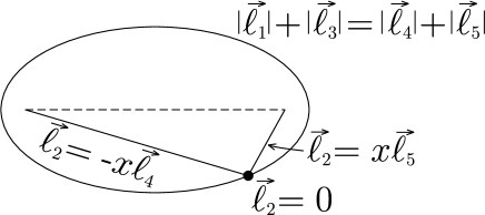
FIG. 6.: Locations of singularities of ${\cal G}_{a}$.

A The collinear singularities

In this subsection, we examine the collinear singularity at $\vec{\ell}_{2}=-x\vec{\ell}_{4}$ with $0<x<1$. The principles that we discover for this case will hold for the other collinear singularities as well.

The terms ${\cal G}_{a1}$ and ${\cal G}_{c}$ in the integrand ${\cal G}$, Eq. (20), are singular along the line $\vec{\ell}_{2}=-x\vec{\ell}_{4}$, $0<x<1$. In order to examine this singularity, let us write ${\cal G}_{a1}$ and ${\cal G}_{c}$ as given in Eq. (28) in the form

$${\cal G}_{a1}={1\over 2|\vec{\ell}_{2}+\vec{\ell}_{4}|}\ {1\over\left(E_{2}^{(a1)}\right)^{2}-\vec{\ell}_{2}^{\,2}}\ {1\over 2|\vec{\ell}_{4}|}\ {\cal R}(E_{1},E_{2}^{(a1)},E_{5},\vec{\ell}_{2},\vec{\ell}_{4})\ {\cal S}_{2}(\vec{\ell}_{4},\vec{q}-\vec{\ell}_{4}),$$ (29)

$${\cal G}_{c}={1\over 2|\vec{\ell}_{2}+\vec{\ell}_{4}|}\ {1\over 2|\vec{\ell}_{2}|}\ {1\over\left(E_{1}-E_{2}^{(c)}\right)^{2}-\vec{\ell}_{4}^{\,2}}\ {\cal R}(E_{1},E_{2}^{(c)},E_{5},\vec{\ell}_{2},\vec{\ell}_{4})\ {\cal S}_{3}(\vec{\ell}_{1},-\vec{\ell}_{2},\vec{q}-\vec{\ell}_{4}).$$ (30)

Here the first factors exhibit the denominators for the three propagators that carry collinear momenta at the singularity, ${\cal R}$ denotes the rest of the Feynman graph, and the ${\cal S}$ functions are the measurement functions for the final state particles. The functions ${\cal R}$ depend on the loop momenta $\vec{\ell}_{2}$ and $\vec{\ell}_{4}$ and on three loop energies, which we take to be $E_{1}=\ell_{1}^{0}$, $E_{2}=\ell_{2}^{0}$ and $E_{5}=\ell_{5}^{0}$. The energies are determined by the on-shell delta functions for the two contributions. For $E_{1}$ and $E_{5}$, the values are the same for the two contributions:

$$E_{1} = |\vec{\ell}_{2}+\vec{\ell}_{4}|,$$ (31)

$$E_{5} = |\vec{q}-\vec{\ell}_{4}|.$$ (32)

For $E_{2}$, the values are different:

$$E_{2}^{(a1)} = |\vec{\ell}_{2}+\vec{\ell}_{4}|-|\vec{\ell}_{4}|,$$ (33)

$$E_{2}^{(c)} = -|\vec{\ell}_{2}|.$$ (34)

In order to examine the behavior of ${\cal G}_{a1}$ and ${\cal G}_{c}$ near the singularity, let

$$\vec{\ell}_{2}=-x\vec{\ell}_{4}+\vec{\ell}_{T},$$ (35)

where $\vec{\ell}_{T}\cdot\vec{\ell}_{4}=0$. The singularity is at $\vec{\ell}_{T}\to 0$.

In ${\cal G}_{a1}$ the denominator $\left(E_{2}^{(a1)}\right)^{2}-\vec{\ell}_{2}^{\,2}$ vanishes at $\vec{\ell}_{T}\to 0$:

$$\left(E_{2}^{(a1)}\right)^{2}-\vec{\ell}_{2}^{\,2}=-{\vec{\ell}_{T}^{\,2}\over 1-x}\left(1+{\cal O}(\vec{\ell}_{T}^{\,2})\right).$$ (36)

Thus there is a $1/\vec{\ell}_{T}^{\,2}$ singularity which would give a logarithmically divergent result for the integral of ${\cal G}_{a1}$ alone. Altogether, the denominator factors for ${\cal G}_{a1}$ are

$${1\over 2|\vec{\ell}_{2}+\vec{\ell}_{4}|}\ {1\over\left(E_{2}^{(a1)}\right)^{2}-\vec{\ell}_{2}^{\,2}}\ {1\over 2|\vec{\ell}_{4}|}\ =-{1\over 4\vec{\ell}_{4}^{\,2}}\ {1\over\vec{\ell}_{T}^{\,2}}\ \left(1+{\cal O}(\vec{\ell}_{T}^{\,2})\right).$$ (37)

Let us now look at the denominator factors for ${\cal G}_{c}$. The denominator $\left(E_{1}-E_{2}^{(c)}\right)^{2}-\vec{\ell}_{4}^{\,2}$ takes the form

$$\left(\left(E_{1}-E_{2}^{(c)}\right)^{2}-\vec{\ell}_{4}^{\,2}\right)^{2}={\vec{\ell}_{T}^{\,2}\over x(1-x)}\left(1+{\cal O}(\vec{\ell}_{T}^{\,2})\right),$$ (38)

so that the denominator factors together take the form

$${1\over 2|\vec{\ell}_{2}+\vec{\ell}_{4}|}\ {1\over 2|\vec{\ell}_{2}|}\ {1\over\left(E_{1}-E_{2}^{(c)}\right)^{2}-\vec{\ell}_{4}^{\,2}}\ ={1\over 4\vec{\ell}_{4}^{\,2}}\ {1\over\vec{\ell}_{T}^{\,2}}\ \left(1+{\cal O}(\vec{\ell}_{T}^{\,2})\right).$$ (39)

Again, we have a $1/\vec{\ell}_{T}^{\,2}$ singularity.

Note, however, that the denominator factors in Eqs. (37) and (39) are equal except for their sign, up to corrections that are not singular as $\vec{\ell}_{T}^{\,2}\to 0$. Thus if the remaining factors ${\cal R}$ and ${\cal S}$ were exactly the same for ${\cal G}_{a1}$ and ${\cal G}_{c}$ there would be no singularity in their sum.

We thus need to explore the matching of ${\cal R}$ and ${\cal S}$. The two versions of ${\cal R}$ are the same functions with the same arguments except for the fact that $E_{2}^{(c)}\neq E_{2}^{(a1)}$. However,

$$E_{2}^{(c)}=E_{2}^{(a1)}+{\cal O}(\vec{\ell}_{T}^{\,2}).$$ (40)

Thus

$${\cal R}(E_{1},E_{2}^{(c)},E_{5},\vec{\ell}_{2},\vec{\ell}_{4})={\cal R}(E_{1},E_{2}^{(a1)},E_{5},\vec{\ell}_{2},\vec{\ell}_{4})+{\cal O}(\vec{\ell}_{T}^{\,2}).$$ (41)

For the functions $\cal S$ used in our example, we have

$${\cal S}_{3}((1-x)\vec{\ell}_{4}+\vec{\ell}_{T},x\vec{\ell}_{4}-\vec{\ell}_{T},\vec{q}-\vec{\ell}_{4})={\cal S}_{2}(\vec{\ell}_{4},\vec{q}-\vec{\ell}_{4})+{\cal O}(\vec{\ell}_{T}^{\,2}).$$ (42)

Using these matching equations we find that

$${\cal G}_{a1}+{\cal G}_{c}={\cal O}(1)$$ (43)

as $\vec{\ell}_{T}\to 0$. There is no collinear singularity in $\cal G$.

How general is this result? First of all note that, in the part of the argument not involving the measurement functions ${\cal S}$, we used only the explicit structure of the denominators for three propagators that meet at a vertex. In the limit in which the momenta carried on these propagators become collinear, there is a cancellation of the collinear singularity arising from these denominators. The three propagators can be part of a much larger graph, and there can be non-trivial numerator factors, as in QCD. All of the other factors can be lumped into a function ${\cal R}$ and treated as above. Thus this cancellation works in QCD as well as $\phi^{3}$ theory and it works for cut graphs with at most one virtual loop at any order of perturbation theory.

As for the measurement functions, in general we need to consider the difference between the measurement functions with $n$ and $n+1$ particles in the final state,

$$F(\vec{\ell}_{T})={\cal S}_{n+1}(\vec{k}_{1},\cdots,\vec{k}_{n-1},x\vec{k}_{n}-\vec{\ell}_{T},(1-x)\vec{k}_{n}+\vec{\ell}_{T})-{\cal S}_{n}(\vec{k}_{1},\cdots,\vec{k}_{n-1},\vec{k}_{n}).$$ (44)

Assuming that $F$ is an analytic function of $\vec{\ell}_{T}$, it will have an expansion around $\vec{\ell}_{T}=0$ of the form

$$F(\vec{\ell}_{T})=a+b_{i}\cdot\ell_{T}^{i}+c_{ij}\ell_{T}^{i}\ell_{T}^{j}+\cdots.$$ (45)

Infrared safety requires that $a=0$. If $b_{i}\neq 0$ then $F$ vanishes on a surface that intersects the point $\vec{\ell}_{T}=0$. Measurement functions ${\cal S}$ with this property would define an infrared safe measurement, but I do not know of any example in common use. More typically, $F$ is non-zero in a neighborhood of $\vec{\ell}_{T}=0$ while vanishing at $\vec{\ell}_{T}=0$. Then both $a$ and the $b_{i}$ must vanish and the $c_{ij}$ should be a positive definite (or negative definite) matrix. Thus, for typical measurement functions,

$$F(\vec{\ell}_{T})={\cal O}(\vec{\ell}_{T}^{\,2})$$ (46)

as $\vec{\ell}_{T}\to 0$. Then the integrand does not have collinear singularities.

For an atypical measurement function with $b_{i}\neq 0$, one would be left with an integrable singularity of the form $\vec{b}\cdot\vec{\ell}_{T}/\vec{\ell}_{T}^{\,2}$. The current version of the computer code [3] has a mechanism to deal with this contingency, but I do not discuss it here since I know of no case in which it is needed.

B The soft singularities

In this subsection, we examine the soft singularity at $\vec{\ell}_{2}=0$.

Let us concentrate to begin with on the cut graph shown in Fig. 3(a). When we perform the integration over the energy circulating in the virtual loop, there is a contribution from the term in which the propagator carrying momentum $\ell_{1}^{\mu}$ is put on shell, as in Fig. 4(a1). This contribution is ${\cal G}_{a1}$ in Eq. (28). Let us examine this contribution in the limit $\vec{\ell}_{2}\to 0$. Expanding in powers of $\vec{\ell}_{2}$, we have

$$\ell_{1}^{0}=|\vec{\ell}_{1}|=|\vec{\ell}_{4}+\vec{\ell}_{2}|=|\vec{\ell}_{4}|+|\vec{\ell}_{2}|\,\vec{u}_{2}\cdot\vec{u}_{4}+\cdots,$$ (47)

where we adopt the notation

$$\vec{u}_{J}=\vec{\ell}_{J}/|\vec{\ell}_{J}|.$$ (48)

Then

$$\ell_{2}^{2}=-|\vec{\ell}_{2}|^{2}\ [1-(\vec{u}_{2}\cdot\vec{u}_{4})^{2}]+\cdots$$ (49)

and

$$\ell_{3}^{2}=2|\vec{\ell}_{5}|\,|\vec{\ell}_{2}|\ \vec{u}_{2}\cdot(\vec{u}_{5}-\vec{u}_{4})+\cdots.$$ (50)

Thus

$${\cal G}_{a1} \sim {\cal S}_{2}\,{1\over 2|\vec{\ell}_{4}|}\,{-1\over|\vec{\ell}_{2}|^{2}\ [1-(\vec{u}_{2}\cdot\vec{u}_{4})^{2}]}\,{1\over 2|\vec{\ell}_{5}|\,|\vec{\ell}_{2}|\ \vec{u}_{2}\cdot(\vec{u}_{5}-\vec{u}_{4})+i\epsilon}\,{1\over 2|\vec{\ell}_{4}|}\,{1\over 2|\vec{\ell}_{5}|}$$ (51)

$$= {{\cal S}_{2}\over 16\,|\vec{\ell}_{4}|^{2}\,|\vec{\ell}_{5}|^{2}}\,{1\over|\vec{\ell}_{2}|^{3}}\,{1\over 1-(\vec{u}_{2}\cdot\vec{u}_{4})^{2}}\,{1\over\vec{u}_{2}\cdot(\vec{u}_{5}-\vec{u}_{4})+i\epsilon}.$$ (52)

We proceed in this fashion to evaluate the contribution corresponding to Fig. 4(a2). Then we evaluate the contribution of Fig. 4(a3), but we find that this contribution is not singular as $\vec{\ell}_{2}\to 0$. Adding the three contributions, we obtain the net integrand for the cut graph of Fig. 3(a) in the soft limit $\vec{\ell}_{2}\to 0$:

$${\cal G}_{a}\sim{-{\cal S}_{2}\over 32\,|\vec{\ell}_{4}|^{2}\,|\vec{\ell}_{5}|^{2}}\,{1\over|\vec{\ell}_{2}|^{3}}\,{1\over 1+\vec{u}_{2}\cdot\vec{u}_{4}}\,{1\over 1-\vec{u}_{2}\cdot\vec{u}_{5}}\,{2-\vec{u}_{2}\cdot(\vec{u}_{5}-\vec{u}_{4})\over\vec{u}_{2}\cdot(\vec{u}_{5}-\vec{u}_{4})+i\epsilon}.$$ (53)

Some comments are in order here. First, we have included the leading term, with a $1/|\vec{\ell}_{2}|^{3}$ singularity, and dropped less singular terms. If we decompose the integration over $\vec{\ell}_{2}$ into $\int\!d\Omega_{2}\,\int|\vec{\ell}_{2}|^{2}d|\vec{\ell}_{2}|$, then a $1/|\vec{\ell}_{2}|^{3}$ singularity produces a logarithmic divergence in the integration over $|\vec{\ell}_{2}|$. The less singular terms will lead to a finite integration over $|\vec{\ell}_{2}|$, although the integration $\int\!d\Omega$ over the angles $\vec{u}_{2}$ can still be divergent. There are, in fact, singularities in the angular integration. The factor $1/[1-\vec{u}_{2}\cdot\vec{u}_{5}]$ is singular when $\vec{\ell}_{2}$ is collinear with $\vec{\ell}_{5}$, while the factor $1/[1+\vec{u}_{2}\cdot\vec{u}_{4}]$ is singular when $-\vec{\ell}_{2}$ is collinear with $\vec{\ell}_{4}$. These singularities produce logarithmically divergent integrations over $\vec{u}_{2}$. However, the analysis of the previous subsection shows that the collinear singularities cancel among the cuts of our graph. There is also a singularity on the plane $\vec{u}_{2}\cdot(\vec{u}_{5}-\vec{u}_{4})=0$. This is the scattering singularity on the ellipse $|\vec{\ell}_{1}|+|\vec{\ell}_{3}|=|\vec{\ell}_{4}|+|\vec{\ell}_{5}|$. This ellipse passes through the point $\vec{\ell}_{2}=0$ and the plane tangent to the ellipse at this point is the plane $\vec{u}_{2}\cdot(\vec{u}_{5}-\vec{u}_{4})=0$. I will have more to say about this singularity later. Here we note simply that it comes with an $i\epsilon$ prescription, which has been preserved in Eq. (53).

We now consider the cut graph shown in Fig. 3(b). Again, there are three contributions to consider, corresponding to the diagrams $(b5)$, $(b2)$ and $(b4)$ in Fig. 4. Adding the three contributions, we obtain the net integrand for the cut graph of Fig. 3(b) in the soft limit $\vec{\ell}_{2}\to 0$:

$${\cal G}_{b}\sim{{\cal S}_{2}\over 32\,|\vec{\ell}_{4}|^{2}\,|\vec{\ell}_{5}|^{2}}\,{1\over|\vec{\ell}_{2}|^{3}}\,{1\over 1-\vec{u}_{2}\cdot\vec{u}_{4}}\,{1\over 1+\vec{u}_{2}\cdot\vec{u}_{5}}\,{2+\vec{u}_{2}\cdot(\vec{u}_{5}-\vec{u}_{4})\over\vec{u}_{2}\cdot(\vec{u}_{5}-\vec{u}_{4})+i\epsilon}.$$ (54)

As in Eq. (53), there are a scattering singularity and two collinear singularities. However, the signs that indicate the location of the collinear singularities are reversed compared to Eq. (54). If we add ${\cal G}_{a}$ and ${\cal G}_{b}$ we obtain

$${\cal G}_{a}+{\cal G}_{b}\sim{-{\cal S}_{2}\over 16\,|\vec{\ell}_{4}|^{2}\,|\vec{\ell}_{5}|^{2}}\,{1\over|\vec{\ell}_{2}|^{3}}\,{1+(\vec{u}_{2}\cdot\vec{u}_{4})(\vec{u}_{2}\cdot\vec{u}_{5})\over[1-(\vec{u}_{2}\cdot\vec{u}_{4})^{2}][1-(\vec{u}_{2}\cdot\vec{u}_{5})^{2}]}.$$ (55)

Thus, the overall $1/|\vec{\ell}_{2}|^{3}$ singularity remains and the collinear singularities remain, but the scattering singularities cancel in the soft limit, $\vec{\ell}_{2}\to 0$, between the two cuts that leave virtual subgraphs.

There are two more cut graphs to consider. The graph shown in Fig. 3(c) gives

$${\cal G}_{c}\sim{{\cal S}_{3}\over 32\,|\vec{\ell}_{4}|^{2}\,|\vec{\ell}_{5}|^{2}}\,{1\over|\vec{\ell}_{2}|^{3}}\,{1\over[1+\vec{u}_{2}\cdot\vec{u}_{4}]}\,{1\over[1+\vec{u}_{2}\cdot\vec{u}_{5}]}.$$ (56)

The graph shown in Fig. 3(d) gives

$${\cal G}_{d}\sim{{\cal S}_{3}\over 32\,|\vec{\ell}_{4}|^{2}\,|\vec{\ell}_{5}|^{2}}\,{1\over|\vec{\ell}_{2}|^{3}}\,{1\over[1-\vec{u}_{2}\cdot\vec{u}_{4}]}\,{1\over[1-\vec{u}_{2}\cdot\vec{u}_{5}]}.$$ (57)

Adding these together, we find

$${\cal G}_{c}+{\cal G}_{d}\sim{{\cal S}_{3}\over 16\,|\vec{\ell}_{4}|^{2}\,|\vec{\ell}_{5}|^{2}}\,{1\over|\vec{\ell}_{2}|^{3}}\,{1+(\vec{u}_{2}\cdot\vec{u}_{4})(\vec{u}_{2}\cdot\vec{u}_{5})\over[1-(\vec{u}_{2}\cdot\vec{u}_{4})^{2}][1-(\vec{u}_{2}\cdot\vec{u}_{5})^{2}]}.$$ (58)

We note that when we add the contributions of the cuts which leave virtual subgraphs to the contributions of the cuts which have no virtual subgraphs, the leading soft singularity cancels:

$${\cal G}_{a}+{\cal G}_{b}+{\cal G}_{c}+{\cal G}_{d}\sim 0.$$ (59)

That is, after cancellation, the overall singularity is at worst proportional to $1/|\vec{\ell}_{2}|^{2}$. It is thus an integrable singularity provided that all of the singularities of the angular integration over $\vec{u}_{2}$ cause no problems.

The cancellation of the leading soft singularity is built into the structure of Feynman diagrams, so that we do not have to do anything special to make it happen. However, there is a certain subtlety in arranging for the singularities in the angular integrations to be convergent in a Monte Carlo integration. Thus, we will return to the cancellation of the soft singularity after we have discussed contour deformations in the following section.

V The scattering singularity and contour deformation

Consider the contribution from Fig. 4(a1), as given in Eq. (28). There is a factor

$${1\over(|\vec{\ell}_{1}|-|\vec{\ell}_{4}|-|\vec{\ell}_{5}|)^{2}-\vec{\ell}_{3}^{\,2}+i\epsilon}={1\over(|\vec{\ell}_{3}|+|\vec{\ell}_{4}|+|\vec{\ell}_{5}|-|\vec{\ell}_{1}|)(|\vec{\ell}_{4}|+|\vec{\ell}_{5}|-|\vec{\ell}_{1}|-|\vec{\ell}_{3}|+i\epsilon)},$$ (60)

which has a singularity when $|\vec{\ell}_{1}|+|\vec{\ell}_{3}|=|\vec{\ell}_{4}|+|\vec{\ell}_{5}|$. In an analysis using time-ordered perturbation theory, the singular factor emerges from the energy denominator associated with the intermediate state consisting of partons 1 and 3,

$$E_{F}-E(\vec{\ell}_{2})+i\epsilon,$$ (61)

where $E_{F}=|\vec{\ell}_{4}|+|\vec{\ell}_{5}|$ and

$$E(\vec{\ell}_{2})=|\vec{\ell}_{1}|+|\vec{\ell}_{3}|=|\vec{\ell}_{4}+\vec{\ell}_{2}|+|-\vec{\ell}_{5}+\vec{\ell}_{2}|.$$ (62)

Thus the singularity appears when the momenta are right for particles 1 and 3 to be on-shell and scatter to produce the final state particles 4 and 5.

The contribution from Fig. 4(b4) has a scattering singularity at the same place as that from the cut diagram (a1). However, these singularities do not cancel in general because the functions ${\cal S}_{2}(\vec{\ell}_{4},\vec{\ell}_{5})$ and ${\cal S}_{2}(\vec{\ell}_{1},\vec{\ell}_{3})$ do not match. We thus have a problem if we would like to perform the integration numerically.

We notice, however, that the singularity is protected by an $i\epsilon$ prescription. The $i\epsilon$ in the denominator tells us what to do in an analytic calculation and it also tells us what to do in a numerical calculation: we need to deform the integration contour.

We are integrating over a loop momentum $\vec{\ell}_{2}$. Let us replace $\vec{\ell}_{2}$ by a complex momentum $\vec{\ell}_{2,c}=\vec{\ell}_{2}+i\vec{\kappa}$, where $\vec{\kappa}$ is a function, which remains to be determined, of $\vec{\ell}_{2}$. Then as we integrate over the real vector $\vec{\ell}_{2}$, we are integrating over a contour in the space of the complex vector $\vec{\ell}_{2,c}$. When we deform the original contour $\vec{\ell}_{2,c}=\vec{\ell}_{2}$ to the new contour $\vec{\ell}_{2,c}=\vec{\ell}_{2}+i\vec{\kappa}$, the integral does not change provided that we do not cross any points where the integrand is singular and provided that we include a jacobian

$${\cal J}(\vec{\ell}_{2})=\det\left(\partial\ell_{2,c}^{i}\over\partial\ell_{2}^{j}\right).$$ (63)

There are some subtleties associated with this; the relevant theorem is proved in the Appendix.

We need to choose $\vec{\kappa}$ as a function of $\vec{\ell}_{2}$. Consider first the direction of $\vec{\kappa}$. On the deformed contour, the energy denominator (61) has the form

$$E_{F}-E(\vec{\ell}_{2}+i\vec{\kappa})+i\epsilon.$$ (64)

In order to fix the direction of deformation, it is useful to consider what happens when we deform the contour just a little way from the real $\vec{\ell}_{2}$ space. For small $\kappa$, we have

$$E(\vec{\ell}_{2}+i\vec{\kappa})\approx|\vec{\ell}_{1}|+|\vec{\ell}_{3}|+i\vec{\kappa}\cdot\vec{w},$$ (65)

where

$$\vec{w}={\vec{\ell}_{1}\over|\vec{\ell}_{1}|}+{\vec{\ell}_{3}\over|\vec{\ell}_{3}|}.$$ (66)

Thus the energy denominator is ${E_{F}-E(\vec{\ell}_{2})-i\vec{\kappa}\cdot\vec{w}+i\epsilon}$ for small $\vec{\kappa}$. In order to keep on the proper side of the singularity, we want $\vec{\kappa}\cdot\vec{w}$ to be negative. The simplest way to insure this is to choose $\vec{\kappa}$ in the direction of $-\vec{w}$. Thus we choose

$$\vec{\kappa}=-D(\vec{\ell}_{2})\,\vec{w},\hskip 28.45274ptD(\vec{\ell}_{2})\geq 0.$$ (67)

Then the singular factor is approximately

$${1\over E_{F}-E(\vec{\ell}_{2})+iD(\vec{\ell}_{2})\,\vec{w}^{\,2}}$$ (68)

for a small deformation. For a larger deformation, it not so simple to see that we stay on the correct side of the singularity, but it is easy to check numerically.

The next question is how should we choose $D(\vec{\ell}_{2})$? We want $D$ not to be small when $\vec{\ell}_{2}$ is near the surface $E(\vec{\ell}_{2})=E_{F}$ in order that the integrand not be large there. We want $D(\vec{\ell}_{2})$ not to grow as $\vec{\ell}_{2}^{\,2}\to\infty$ in order to satisfy the conditions for the theorem that deforming the contour does not change value of the integral. Since there is no reason to keep any finite contour deformation for large $\vec{\ell}_{2}^{\,2}$, we will simply choose to have $D(\vec{\ell}_{2})\to 0$ as $\vec{\ell}_{2}^{\,2}\to\infty$.

There is another condition that $D(\vec{\ell}_{2})$ should obey: it should vanish at points where ${\cal G}$ has collinear and soft singularities. To see why takes some discussion.

Consider the contributions from three parton cuts, for which there is no virtual loop. For these contributions, we do not want to deform the contours. This is because if any of the loop momenta were complex then at least one of the momenta of the final state particles would be complex. In principle, one could have complex momenta for final state particles as long as the measurement functions ${\cal S}_{n}(\vec{k}_{1},\dots,\vec{k}_{n})$ are analytic. However, I have in mind applications in which the numerical integration program acts as a subroutine that produces “events” with final state particle momenta $\{\vec{k}_{1},\dots,\vec{k}_{n}\}$ and weights computed by the subroutine. Then the events could be the input to, for example, a Monte Carlo program that generates parton showers and hadronization. Surely complex momenta for the final state particles are not desirable.

Now recall that there is a cancellation among the contributions ${\cal G}_{C}$ from different cuts $C$ at points where the ${\cal G}_{C}$ have collinear and soft singularities. Evidently, if we deform the contour for a contribution with a virtual graph but do not deform the contour for the canceling contribution, then the cancellation can be spoiled. We can avoid spoiling the cancellation if we make the contours match at the singularity. That is, $D(\vec{\ell}_{2})$ should vanish at the points where the ${\cal G}_{C}$ have collinear and soft singularities.

We also need to determine how fast $D(\vec{\ell}_{2})$ needs to approach zero as $\vec{\ell}_{2}$ approaches a singularity. Since the integration is in a multidimensional complex space, we need an analysis that makes use of the multidimensional contour deformation theorem. This analysis is given in the Appendix. Here, I present a simpler one dimensional analysis that can serve to clarify the issue.

Consider the following toy integral,

$$I=\int_{0}^{x_{\rm max}}{dx\over x}\ \left\{{f_{V}(x)\over x-1+i\epsilon}+f_{R}(x)\right\}.$$ (69)

Here the endpoint singularity at $x=0$ plays the role of the collinear or soft singularities. The function $f_{V}/(x-1+i\epsilon)$ plays the role of the integrand for the contribution with a virtual subgraph. In this contribution, there is a singularity at $x=1$ that comes with an $i\epsilon$ prescription. The function $f_{R}$ plays the role of the integrand for the contribution with no virtual subgraph. We assume that $f_{V}(z)$ and $f_{R}(z)$ are analytic functions. We also assume that $f_{V}(0)=f_{R}(0)$, so that the apparent singularity at $x=0$ cancels.

Now the $i\epsilon$ prescription on the singularity at $x=1$ tells us that we can deform the integration contour into the upper half plane, replacing $x$ by $z=x+iy(x)$ where $y(0)=y(x_{\rm max})=0$. Thus

$$I=\int_{0}^{x_{\rm max}}\!dx\ {1+iy^{\prime}(x)\over x+iy(x)}\ \ \left\{{f_{V}\left(x+iy(x)\right)\over x-1+iy(x)}+f_{R}\left(x+iy(x)\right)\right\}.$$ (70)

Suppose, however, that we want to keep the contour for $f_{R}$ on the real axis. Then we might hope that $I=\tilde{I}$, where

$$\tilde{I}=\lim_{x_{\rm min}\to 0}\int_{x_{\rm min}}^{x_{\rm max}}\!dx\ \left\{{1+iy^{\prime}(x)\over x+iy(x)}\ {f_{V}\left(x+iy(x)\right)\over x-1+iy(x)}+{f_{R}\left(x\right)\over x}\right\}.$$ (71)

The difference is

$$\tilde{I}-I=\lim_{x_{\rm min}\to 0}\int_{x_{\rm min}}^{x_{\rm max}}\!dx\ \left\{{f_{R}\left(x\right)\over x}-[1+iy^{\prime}(x)]{f_{R}\left(x+iy(x)\right)\over x+iy(x)}\ \right\}.$$ (72)

If we note that $[f_{R}(z)-f_{R}(0)]/z$ is an analytic function even at $z=0$ and that the integral of an analytic function around a closed contour vanishes, we have

$$0=\lim_{x_{\rm min}\to 0}\int_{x_{\rm min}}^{x_{\rm max}}\!dx\ \left\{{f_{R}\left(x\right)-f_{R}\left(0\right)\over x}-[1+iy^{\prime}(x)]{f_{R}\left(x+iy(x)\right)-f_{R}\left(0\right)\over x+iy(x)}\ \right\}.$$ (73)

Subtracting these and performing the integral, we have

$$\tilde{I}-I=f_{R}(0)\ \lim_{x_{\rm min}\to 0}\int_{x_{\rm min}}^{x_{\rm max}}\!dx\ \left\{{1\over x}-{1+iy^{\prime}(x)\over x+iy(x)}\ \right\}=f_{R}(0)\ \lim_{x_{\rm min}\to 0}\log\left(1+i\,{y(x_{\rm min})\over x_{\rm min}}\right).$$ (74)

We can draw two conclusions. First, as long as $y(x)\to 0$ at least as fast as $x^{1}$ as $x\to 0$, we will realize the cancellation of the $x\to 0$ singularity and obtain a finite value for $\tilde{I}$. Second, if we choose $y(x)\propto x$ as $x\to 0$, $\tilde{I}$ will be finite, but it will not be equal to the correct result $I$. In order to get a result $\tilde{I}$ that is not only finite but also correct, we need $y(x)/x\to 0$ as $x\to 0$. A convenient choice is $y(x)\propto x^{2}$ as $x\to 0$.

We conclude from the multidimensional extension of this analysis, given in the Appendix, that as $\vec{\ell}_{2}$ approaches a singularity, $D(\vec{\ell}_{2})$ should approach zero quadratically with the distance to the singularity.

We now use the qualitative criteria just developed to give a specific choice of deformation. We have chosen

$$\vec{\ell}_{2,c}=\vec{\ell}_{2}-iD(\vec{\ell}_{2})\vec{w},$$ (75)

where $\vec{w}$, Eq. (66), specifies the direction of deformation. We now specify a deformation function $D(\vec{\ell}_{2})$ that satisfies our criteria. We write $D$ in the form

$$D=C\,G.$$ (76)

The factor $C$ is designed to insure that the deformation vanishes quadratically near the collinear and soft singularities. The factor $G$ is designed to turn the deformation off for large $\vec{\ell}_{2}$. These factors are explained below and are defined precisely in Eqs. (80) and (83) below.

First, we discuss the factor $C$. We want the deformation to vanish at the line $\vec{\ell}_{2}=-x\vec{\ell}_{4}$ with $0\leq x\leq 1$, where the amplitude has a collinear singularity. (Since $\vec{\ell}_{4}=\vec{\ell}_{1}-\vec{\ell}_{2}$, this line is also $\vec{\ell}_{1}=-\lambda\vec{\ell}_{2}$ with $0<\lambda<\infty$.) Define

$$d_{12}={\left||\vec{\ell}_{2}|\vec{\ell}_{1}+|\vec{\ell}_{1}|\vec{\ell}_{2}\right|\over|\vec{\ell}_{1}-\vec{\ell}_{2}|}={\left||\vec{\ell}_{2}|\vec{\ell}_{1}+|\vec{\ell}_{1}|\vec{\ell}_{2}\right|\over|\vec{\ell}_{4}|}.$$ (77)

This function is zero on the line $\vec{\ell}_{2}=-x\vec{\ell}_{4}$ with $0\leq x\leq 1$, and furthermore, it vanishes linearly as $\vec{\ell}_{2}$ approaches this line. Similarly, we want the deformation to vanish on the line $\vec{\ell}_{2}=x\vec{\ell}_{5}$ with $0\leq x\leq 1$, where the amplitude has its other collinear singularity. The function $d_{23}$, where

$$d_{23}={\left||\vec{\ell}_{3}|\vec{\ell}_{2}+|\vec{\ell}_{2}|\vec{\ell}_{3}\right|\over|\vec{\ell}_{2}-\vec{\ell}_{3}|}={\left||\vec{\ell}_{3}|\vec{\ell}_{2}+|\vec{\ell}_{2}|\vec{\ell}_{3}\right|\over|\vec{\ell}_{5}|},$$ (78)

vanishes linearly as $\vec{\ell}_{2}$ approaches this line. (To see this, use $\vec{\ell}_{5}=\vec{\ell}_{2}-\vec{\ell}_{3}$.) Let

$$d=\min(d_{12},d_{23}).$$ (79)

Then $d$ vanishes linearly with the distance to either of the collinear singularities. It also vanishes linearly with the distance to the soft singularity at $\vec{\ell}_{2}=0$.

Now, we have seen that the deformation should vanish quadratically with the distance to any of the singularities. We can achieve this by letting

$$C(d^{2})={\alpha\,d^{2}\over 1+4\beta d^{2}/(|\ell_{4}|+|\ell_{5}|+|\vec{q}|)^{2}},$$ (80)

where $\alpha$ and $\beta$ are adjustable dimensionless parameters. Note that, for large $d$, $C(d^{2})$ approaches a constant.

Next, we discuss the factor $G$. We want to ensure that the contour deformation vanishes for large $\vec{\ell}_{2}$. Let us define

$$a=|\vec{\ell}_{1}|+|\vec{\ell}_{3}|-|\vec{q}|$$ (81)

and

$$A=|\vec{\ell}_{4}|+|\vec{\ell}_{5}|-|\vec{q}|.$$ (82)

Then the singularity that we are avoiding by means of contour deformation is at $a=A$. We can turn the deformation off for $a\gg A$ by setting

$$G(a)={1\over A+\gamma a},$$ (83)

where $\gamma$ is an adjustable dimensionless parameter.

There is a subsidiary reason for this choice. At the singularity, $G=1/[(1+\gamma)A]$. The factor $1/A$ serves to enhance the deformation in the case that $\vec{\ell}_{4}$ and $\vec{\ell}_{5}$ are nearly collinear, in which case $d$ is small on the ellipse $a=A$ and the deformation would otherwise be too small.

The reader will note that, while there is a certain uniqueness in defining the direction of the deformation in Eq. (75) to be given by the vector $\vec{w}$, Eq. (66), the normalization $D=C\,G$ with $C$ and $G$ given in Eqs. (80) and (83) is rather ad hoc. Within the requirements that the deformation should vanish quadratically at the collinear and soft singularities and should vanish for large $\vec{\ell}_{2}$, many other choices would be possible. The choice given here is used in the current version of the code [3]. Surely there is some other choice that is better.

VI The Monte Carlo integration

After the contour deformations, we have an integral of the form

$${\cal I}=\int\!d\ell\,\sum_{C}\,{\cal J}(C;\ell)\ g(C;\ell+i\kappa(C;\ell)),$$ (84)

where we use $\ell$ for the loop momenta collectively, $\ell=\{\vec{\ell}_{2},\vec{\ell}_{4}\}$. The index $C$ labels the cut, $a$, $b$, $c$, or $d$ in Fig. 3. There is a contour deformation that depends on the cut, as specified by $\kappa(C;\ell)$, and there is a corresponding jacobian ${\cal J}(C;\ell)$, Eq. (63). Define

$$f(\ell)=\Re\left\{\sum_{C}{\cal J}(C;\ell)\ g(C;\ell+i\kappa(C;\ell))\right\}.$$ (85)

We know that $\cal I$ is real, so

$${\cal I}=\int\!d\ell\,f(\ell).$$ (86)

To perform the integration, we use the Monte Carlo method. We choose points $\ell$ with a density $\rho(\ell)$, with

$$\int\!d\ell\,\rho(\ell)=1.$$ (87)

After choosing $N$ points $\ell_{1},\dots,\ell_{N}$, we have an estimate for the integral:

$${\cal I}\approx{\cal I}_{N}={1\over N}\sum_{i}{f(\ell_{i})\over\rho(\ell_{i})}.$$ (88)

This is an approximation for the integral in the sense that if we repeat the procedure a lot of times the expectation value for ${\cal I}_{N}$ is

$$\langle{\cal I}_{N}\rangle={\cal I}.$$ (89)

The expected r.m.s. error is ${\cal E}$, where

$${\cal E}^{2}=\langle\left({\cal I}_{N}-\cal I\right)^{2}\rangle={1\over N}\int\!d\ell\,{f(\ell)^{2}\over\rho(\ell)}-{{\cal I}^{2}\over N}.$$ (90)

One can rewrite this as

$${\cal E}^{2}={1\over N}\int\!d\ell\,\rho(\ell)\left({|f(\ell)|\over\rho(\ell)}-\tilde{\cal I}\right)^{2}+{\tilde{\cal I}^{2}-{\cal I}^{2}\over N},$$ (91)

where

$$\tilde{\cal I}=\int\!d\ell\,|f(\ell)|.$$ (92)

We see, first of all, that the expected error decreases proportionally to $1/\sqrt{N}$. Second, we see that the ideal choice of $\rho(\ell)$ would be $\rho(\ell)=|f(\ell)|/\tilde{\cal I}$.

Of course, it is not possible to choose $\rho$ in this way. But we know that $|f|$ has singularities at places where propagator momenta vanish and we know the structure of these singularities. We are not really able to choose $\rho$ so that ${|f(\ell)|/\rho(\ell)}$ is a constant, but at least we can choose it so that ${|f(\ell)|/\rho(\ell)}$ is not singular at the singularities of $|f(\ell)|$.

Note that it is easy to combine methods for choosing Monte Carlo points. Suppose that we have a recipe for choosing points with a density $\rho_{1}$ that is singular when one propagator momentum vanishes, a recipe for choosing points with a density $\rho_{2}$ that is singular when another propagator momentum vanishes, and in general recipes for choosing points with densities $\rho_{i}$ with several goals in mind. Then we can devote a fraction $\lambda_{i}$ of the points to the choice with density $\rho_{i}$ and obtain a net density

$$\rho(\ell)=\sum_{i}\lambda_{i}\,\rho_{i}(\ell).$$ (93)

A The density near where a propagator momentum vanishes

Let $\vec{\ell}_{J}$ be the momentum of one of the propagators in our graph. We have seen that when particle $J$ appears in the final state, there is a factor $1/|\vec{\ell}_{J}|$ in the integrand. When propagator $J$ is part of a virtual loop, the contribution corresponding to this propagator being put on shell also contains a factor $1/|\vec{\ell}_{J}|$. Thus there is a singularity $1/|\vec{\ell}_{J}|$ for every propagator in the graph.

The analysis given in the introduction to this section indicates that for each propagator $J$ one of the terms $\rho_{i}$ in the density function should have a singularity that is at least as strong as

$$\rho_{i}(\ell)\propto 1/|\vec{\ell}_{J}|$$ (94)

as $\vec{\ell}_{J}\to 0$. It is, of course, easy to choose points with a density proportional to $1/|\vec{\ell}_{J}|^{A}$ as $\vec{\ell}_{J}\to 0$ as long as $A<3$. (The limitation on $A$ arises because for $A\geq 3$ we would have $\int d\vec{\ell}_{J}\,\rho(\ell)=\infty$.) Thus it is easy to arrange that the density of points has the requisite singularities. Specifically, we can choose $\vec{\ell}_{J}$ with the density

$$\tilde{\rho}(\vec{\ell}_{J})={1\over 2\pi K_{0}^{3}}\ {1\over\left[1+\left(|\vec{\ell}_{J}|/K_{0}\right)^{2}\right]^{2}}\ {K_{0}\over|\vec{\ell}_{J}|},$$ (95)

where $K_{0}$ is a momentum scale determined by the other, previously chosen, loop momenta.

The singularity when $\vec{\ell}_{J}\to 0$ can be more severe than $1/|\vec{\ell}_{J}|$, depending on the structure of the graph. Consider first the cases $J=1,3,4,5$. Here, the singularities for particular cuts, as given in Eq. (28), are $1/|\vec{\ell}_{J}|^{2}$. However, there is a cancellation after one sums over cuts (as for the singularity for $\vec{\ell}_{2}\to 0$), leaving a singularity $1/|\vec{\ell}_{J}|$.

For $J=2$ there is a severe singularity of the form $1/|\vec{\ell}_{J}|^{3}$ for particular contributions to Eq. (28). A $1/|\vec{\ell}_{2}|^{3}$ singularity would not be integrable, but, as we have seen in detail, there is a cancellation among the contributions so that only a $1/|\vec{\ell}_{2}|^{2}$ singularity is left. However, it will not do to simply chose $\rho_{i}(\ell)\propto 1/|\vec{\ell}_{2}|^{2}$ because there is also a singularity in the space of the angles of $\vec{\ell}_{2}$. It is to this subject that we now turn.

B The soft parton singularity

When two partons can scatter by exchanging a parton before they enter the final state, there is a severe singularity as the momentum of the exchanged parton goes to zero. For our graph, this happens for $\vec{\ell}_{2}\to 0$. In this subsection, we consider the behavior of the integrand for small $\vec{\ell}_{2}$ as a function of its magnitude $\vec{\ell}_{2}$ and of its direction $\vec{u}_{2}=\vec{\ell}_{2}/|\vec{\ell}_{2}|$.

The singularity for individual cuts, as given in Eq. (28), is of the form $1/|\vec{\ell}_{2}|^{3}$ when we let $|\vec{\ell}_{2}|\to 0$ with $\vec{u}_{2}$ held fixed. This singularity is not integrable. However, as we have seen, the leading term cancels when we sum over cuts, leaving a $1/|\vec{\ell}_{2}|^{2}$ singularity for $|\vec{\ell}_{2}|\to 0$ with $\vec{u}_{2}$ fixed.

Let us now recall from Eq. (53) that, before we deform the integration contour, the contribution for small $\vec{\ell}_{2}$ from the cut $a$ of Fig. 3 has, in addition to a factor $1/|\vec{\ell}_{2}|^{3}$, a factor $1/[\vec{u}_{2}\cdot(\vec{u}_{5}-\vec{u}_{4})+i\epsilon]$. That is, there is a singularity on a surface in the space of $\vec{\ell}_{2}$ whose tangent plane is the plane perpendicular to $\vec{u}_{5}-\vec{u}_{4}$. We have avoided this singularity by deforming the integration contour. However, the deformation vanishes as $\vec{\ell}_{2}\to 0$. Thus we must face the question of what happens to the cancellation near the soft parton singularity when the contour deformation is taken into account.

First, let us recall from Eq. (75) that for cut $a$ in Fig. 3 the deformation has the form

$$\vec{\ell}_{2,c}=\vec{\ell}_{2}-iD(\vec{\ell}_{2})\,\vec{w},$$ (96)

where $\vec{w}=\vec{u}_{1}+\vec{u}_{3}$. For $\vec{\ell}_{2}\to 0$,

$$\vec{w}\sim\vec{u}_{4}-\vec{u}_{5},$$ (97)

while $D$ has the form

$$D(\vec{\ell}_{2})\sim\vec{\ell}_{2}^{\,2}\ \tilde{D}(\vec{u}_{2}).$$ (98)

Here $\tilde{D}$ vanishes for $\vec{u}_{2}=-\vec{u}_{4}$ and for $\vec{u}_{2}=\vec{u}_{5}$ and is positive elsewhere. Thus

$$\vec{\ell}_{2,c}=|\vec{\ell}_{2}|\left(\vec{u}_{2}+i|\vec{\ell}_{2}|\tilde{D}(\vec{u}_{2})\,(\vec{u}_{5}-\vec{u}_{4})+{\cal O}(\vec{\ell}_{2}^{\,2})\right).$$ (99)

Substituting $\ell_{2,c}$ as given above for $\vec{\ell}_{2}$ in Eq. (53), we obtain an expression for the contribution from cut $a$ to the integrand on the deformed contour near the soft singularity:

$${\cal G}_{a}\sim{-{\cal S}_{2}\over 32\,|\vec{\ell}_{4}|^{2}\,|\vec{\ell}_{5}|^{2}}\,{1\over|\vec{\ell}_{2}|^{3}}\,{1\over 1+\vec{u}_{2}\cdot\vec{u}_{4}}\,{1\over 1-\vec{u}_{2}\cdot\vec{u}_{5}}\,{2-\vec{u}_{2}\cdot(\vec{u}_{5}-\vec{u}_{4})\over\vec{u}_{2}\cdot(\vec{u}_{5}-\vec{u}_{4})+i|\vec{\ell}_{2}|\tilde{D}(\vec{u}_{2})\,(\vec{u}_{5}-\vec{u}_{4})^{2}}.$$ (100)

There are two cases to consider. First, when $|\vec{\ell}_{2}|\to 0$ with $\vec{u}_{2}$ fixed, we can drop the second term in the last denominator. Then ${\cal G}_{a}\sim h(\vec{u}_{2})/|\vec{\ell}_{2}|^{3}$, where the function $h(\vec{u}_{2})$ is the same as on the undeformed contour. As we have seen, the leading $1/|\vec{\ell}_{2}|^{3}$ terms cancel when one sums over cuts. Thus, as noted earlier, the net integrand behaves like

$${\cal G}\sim h_{\rm tot}(\vec{u}_{2})/|\vec{\ell}_{2}|^{2}$$ (101)

when $|\vec{\ell}_{2}|\to 0$ with $\vec{u}_{2}$ fixed.

The second case is more interesting. Consider $|\vec{\ell}_{2}|\to 0$ and $\vec{u}_{2}\cdot(\vec{u}_{5}-\vec{u}_{4})\to 0$ with $\vec{u}_{2}\cdot(\vec{u}_{5}-\vec{u}_{4})/|\vec{\ell}_{2}|$ fixed. Then ${\cal G}_{a}$ is more singular, ${\cal G}_{a}\propto 1/|\vec{\ell}_{2}|^{4}$. To see what happens in this region, we analyze the contribution from cut $b$ in Fig. 3 in the same fashion. The contour deformation for cut $b$ is different from that for cut $a$, but the deformations match at leading order as $|\vec{\ell}_{2}|\to 0$. (This is an important feature of the choice of contour deformations.) Thus we can use Eq. (99) in Eq. (54) to obtain

$${\cal G}_{b}\sim{{\cal S}_{2}\over 32\,|\vec{\ell}_{4}|^{2}\,|\vec{\ell}_{5}|^{2}}\,{1\over|\vec{\ell}_{2}|^{3}}\,{1\over 1-\vec{u}_{2}\cdot\vec{u}_{4}}\,{1\over 1+\vec{u}_{2}\cdot\vec{u}_{5}}\,{2+\vec{u}_{2}\cdot(\vec{u}_{5}-\vec{u}_{4})\over\vec{u}_{2}\cdot(\vec{u}_{5}-\vec{u}_{4})+i|\vec{\ell}_{2}|\tilde{D}(\vec{u}_{2})\,(\vec{u}_{5}-\vec{u}_{4})^{2}}.$$ (102)

We see that ${\cal G}_{b}$ is also proportional to $1/|\vec{\ell}_{2}|^{4}$ in the problematic region. However, since $u_{2}\cdot u_{4}\sim u_{2}\cdot u_{5}$ in this region, the leading $1/|\vec{\ell}_{2}|^{4}$ behavior cancels when we add ${\cal G}_{b}$ to ${\cal G}_{a}$. We are left with the next term, proportional to $1/|\vec{\ell}_{2}|^{3}$.

For the two remaining cuts there is no contour deformation. The contributions from these cuts are each proportional to $1/|\vec{\ell}_{2}|^{3}$. Calculation shows that there is no further cancellation. Thus the net behavior of the integrand is

$${\cal G}\propto 1/|\vec{\ell}_{2}|^{3}$$ (103)

when $|\vec{\ell}_{2}|\to 0$ and $\vec{u}_{2}\cdot(\vec{u}_{5}-\vec{u}_{4})\to 0$ with $\vec{u}_{2}\cdot(\vec{u}_{5}-\vec{u}_{4})/|\vec{\ell}_{2}|$ fixed.

C Density near a soft parton singularity

According to the analysis at the beginning of this section, we should choose a density of integration points that has a singularity that is at least as strong as that of $|{\cal G}|$ near the soft singularity at $\vec{\ell}_{2}\to 0$. Thus we should choose one of the $\rho_{i}$ so that

$$\rho_{i}(\ell) \propto {1\over|\vec{\ell}_{2}|^{p}},\hskip 28.45274pt|\vec{\ell}_{2}|\to 0,\ \vec{u}_{2}\ \ {\rm fixed},$$ (104)

$$\rho_{i}(\ell) \propto {1\over|\vec{\ell}_{2}|^{p+1}},\hskip 28.45274pt|\vec{\ell}_{2}|\to 0,\ {\vec{u}_{2}\cdot(\vec{u}_{5}-\vec{u}_{4})\over|\vec{\ell}_{2}|}\ \ {\rm fixed},$$ (105)

with $p\geq 2$.

Specifically, having chosen $\vec{\ell}_{4}$ we can choose the remaining loop momentum $\vec{\ell}_{2}$ with the density

$$\tilde{\rho}(\vec{\ell}_{2})={1\over 2\pi K_{0}^{3}}\ {1\over\left[1+\left(|\vec{\ell}_{2}|/K_{0}\right)^{(3-p)}\right]^{(5-p)/(3-p)}}\left({K_{0}\over|\vec{\ell}_{2}|}\right)^{p}{1\over\Gamma\sqrt{\cos^{2}(\theta)+\vec{\ell}_{2}^{\,2}/K_{0}^{2}}}.$$ (106)

Here $K_{0}$ is a momentum scale determined by $\vec{\ell}_{4}$, $\theta$ is the angle between $\vec{\ell}_{2}$ and $(\vec{u}_{5}-\vec{u}_{4})$, and

$$\sinh(\Gamma)=K_{0}/|\vec{\ell}_{2}|.$$ (107)

It is easy to choose points with this density by first choosing $|\vec{\ell}_{2}|$, then choosing $\cos(\theta)$, and finally choosing the corresponding azimuthal angle $\phi$ with a uniform density. Accounting for the fact that $\Gamma\propto\log(|\vec{\ell}_{2}|)$ for $\vec{\ell}_{2}\to 0$, we see that $\tilde{\rho}$ will have a singularity stronger than that of ${\cal G}$ provided that $p>2$. We will see how this works in a numerical example in the next section.

VII Numerical Example

In this section, I illustrate the principles developed above by means of a particular example. We consider the integral in Eq. (19). We hold $\vec{\ell}_{4}$ fixed and consider the integrand as a function of $\vec{\ell}_{2}$. In order to simplify the labelling, I define

$$\vec{\ell}_{2}\equiv\vec{\ell}.$$ (108)

There is a contribution for each cut $C$, with $C=a,b,c,\ {\rm or}\ d$. For each contribution from a cut $C$ in which there is a virtual loop, we want to deform the integration contour as discussed in Sec. V. Thus $\vec{\ell}$ gets replaced by a complex vector $\vec{\ell}_{c}=\vec{\ell}+i\vec{\kappa}_{C}$ and we need to supply a jacobian ${\cal J}_{C}(\vec{\ell})$, Eq. (63). Then the integration over $\vec{\ell}$ has the form

$$\int\!d\vec{\ell}\,\sum_{C}{\cal J}_{C}(\vec{\ell})\ {\cal G}_{C}(\vec{\ell}).$$ (109)

The functions ${\cal G}_{C}$ are the analytic continuations to the deformed contours of the functions given in Eq. (28). As discussed in Sec. VI, the quantity that is relevant for the convergence of the Monte Carlo integration is the integrand divided by the density of points chosen for the integration. In this section, I consider only the integration over $\vec{\ell}$, so I discuss a choice for the density of integration points $\rho(\vec{\ell})$ at a fixed $\vec{\ell}_{4}$ and display plots of the functions

$$F_{C}(\vec{\ell})\equiv{1\over\rho(\vec{\ell})}\ {\cal J}_{C}(\vec{\ell})\ {\cal G}_{C}(\vec{\ell})$$ (110)

and $F(\vec{\ell})=\sum_{C}F_{C}(\vec{\ell})$, as well as plots of the deformation and the density.

For the numerical examples, I choose

$$\vec{q}=(3,-0.5,0)$$ (111)

and then take $\vec{\ell}_{4}$ at the point

$$\vec{\ell}_{4}=(2,-1,0).$$ (112)

Since $\vec{\ell}_{5}=\vec{q}-\vec{\ell}_{4}$ we have

$$\vec{\ell}_{5}=(1,0.5,0).$$ (113)

The singularities of the functions ${\cal G}_{C}(\vec{\ell})$ lie in the plane of $\vec{\ell}_{4}$ and $\vec{\ell}_{5}$, that is the $\ell_{z}=0$ plane. In the plots, I choose $\ell_{z}=0$, so that we see the effect of the singularities. I plot $|\vec{\kappa}_{a}|$, $|\vec{\kappa}_{b}|$, $\rho$, $F_{a}$, $F_{b}$, $F_{c}+F_{d}$ and $F$ as functions of $\ell_{x}$ and $\ell_{y}$ in the domain $-2.5<\ell_{x}<1.0$ and $-1.0<\ell_{y}<2.0$.

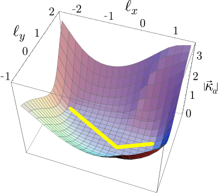
FIG. 7.: Contour deformation for cut $a$. The absolute value of the imaginary part $\vec{\kappa}_{a}$ of $\vec{\ell}_{c}$ for cut $a$ is plotted against $\ell_{x}$ and $\ell_{y}$ at $\ell_{z}=0$. The deformation $\vec{\kappa}_{a}$ vanishes at the two collinear singularities for this cut, which are indicated by lines superimposed on the graph.

Consider first the contour deformation for cut $a$, $\vec{\ell}\to\vec{\ell}_{c}=\vec{\ell}+i\vec{\kappa}_{a}$. I take $\vec{\kappa}_{a}=-D\,\vec{w}$ as given in Eqs. (75-83) with $\alpha=\beta=\gamma=1$. In Fig. 7, I show a graph of $|\vec{\kappa}_{a}|$ versus $\ell_{x}$ and $\ell_{y}$. We see that the deformation is not small. I also display in the figure the lines $\vec{\ell}=-x\vec{\ell}_{4}$ with $0<x<1$ and $\vec{\ell}=x\vec{\ell}_{5}$ with $0<x<1$, where the collinear singularities for cut $a$ are located. We see that, as desired, the deformation vanishes quadratically as $\vec{\ell}$ approaches these lines.

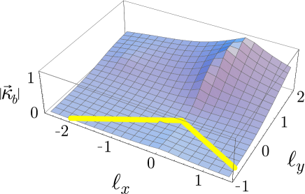
FIG. 8.: Contour deformation for cut $b$. The absolute value of the imaginary part $\vec{\kappa}_{b}$ of $\vec{\ell}_{c}$ for cut $b$ is plotted against $\ell_{x}$ and $\ell_{y}$ at $\ell_{z}=0$. The deformation $\vec{\kappa}_{b}$ vanishes at the two collinear singularities for this cut, which are indicated by lines superimposed on the graph.

There is a different contour deformation for cut $b$. The same formulas apply as for cut $a$ with the replacements $\vec{\ell}_{4}\leftrightarrow\vec{\ell}_{1}$, $\vec{\ell}_{5}\leftrightarrow-\vec{\ell}_{3}$, $\vec{\ell}\leftrightarrow-\vec{\ell}$ and with the sign of $\vec{\kappa}$ reversed. I show a graph of $|\vec{\kappa}_{b}|$ versus $\ell_{x}$ and $\ell_{y}$ in Fig. 8. (This figure does not look like Fig. 7 because $\vec{\ell}$ varies with $\vec{\ell}_{4}$ held fixed, not with $\vec{\ell}_{1}$ held fixed as would be needed if we applied the replacement $\vec{\ell}_{4}\leftrightarrow\vec{\ell}_{1}$ to Fig. 7.) I also display in the figure the lines $\vec{\ell}=\lambda\vec{\ell}_{4}$ with $0<\lambda$ and $\vec{\ell}=-\lambda\vec{\ell}_{5}$ with $0<\lambda$, where the collinear singularities for cut $b$ are located. The deformation vanishes quadratically as $\vec{\ell}$ approaches these lines.

The jacobian functions ${\cal J}_{a}(\vec{\ell})$ and ${\cal J}_{b}(\vec{\ell})$ associated with the contour deformations are quite unremarkable, so I omit showing them.

FIG. 9.: Density of integration points. The density has three singularities. Only values $\rho<1$ are shown.

Consider next the density of integration points. I choose

$$\rho(\vec{\ell})=0.2\,\rho_{1}(\vec{\ell}_{1})+0.6\,\rho_{2}(\vec{\ell})+0.2\,\rho_{3}(\vec{\ell}_{3}),$$ (114)

as shown in Fig. 9. The function $\rho_{1}$ has a mild singularity as $\vec{\ell}_{1}\to 0$ and is given by Eq. (95) with $\vec{\ell}_{1}=\vec{\ell}_{4}-\vec{\ell}$ and with $K_{0}$ set equal to 2. The function $\rho_{3}$ has a mild singularity as $\vec{\ell}_{3}\to 0$; I use the same functional form with $\vec{\ell}_{3}=\vec{\ell}-\vec{\ell}_{5}$. For $\rho_{2}$, I use the function given in Eq. (106) with $K_{0}=2$ and with the power $p$ taken as $p=2.2$. Then $\rho_{2}$ has a strong $1/[|\vec{\ell}|^{2.2}\log(|\vec{\ell}|)]$ singularity as we approach the $\vec{\ell}=0$. Furthermore, the density of points is largest near the plane $\ell_{y}=0$, the plane that is tangent at $\vec{\ell}=0$ to the ellipsoidal surface that (if we turn off the deformation) contains the scattering singularity. In order to display the dependence of $\rho$ on angle near $\vec{\ell}=0$, I plot in Fig. 10 the angle dependent factor in $\rho_{2}$, namely the factor

$${|\vec{\ell}|/K_{0}\over\sqrt{\cos^{2}(\theta)+\vec{\ell}^{\,2}/K_{0}^{2}}}$$ (115)

in Eq. (106), in a region near $\vec{\ell}=0$. Here $\cos(\theta)=\ell_{y}/|\vec{\ell}|$. We see that the density of integration points is heavily concentrated very near the plane $\ell_{y}=0$ when $|\vec{\ell}|$ is small.

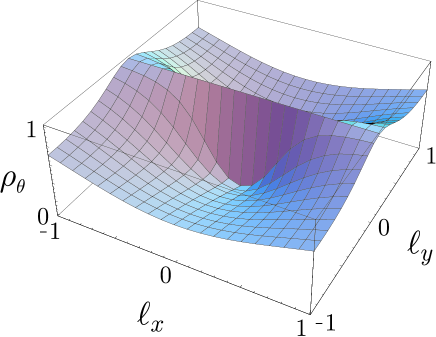
FIG. 10.: Angle dependent factor for the density $\rho_{2}$ of integration points associated with the soft singularity. For small $|\vec{\ell}|$, points are concentrated near $\theta=0$.

We are now ready to look at the contribution $F_{a}={\cal J}_{a}\ {\cal G}_{a}/\rho$ to $F$ from cut $a$. This function is displayed in Fig. 11 with a small rectangle near $\vec{\ell}=0$ removed from the graph. We see the two collinear singularities, at $\vec{\ell}=-x\vec{\ell}_{4}$ and at $\vec{\ell}=x\vec{\ell}_{5}$ with $0<x<1$. As $\vec{\ell}$ approaches one of these singularities, $F_{a}$ approaches $-\infty$.

FIG. 11.: Contribution to $F$ from cut $a$. The domain $-1<\ell_{x}<1$, $-0.3<\ell_{y}<0.3$, which contains the soft singularity, has been removed from the plot in order to make the collinear singularities visible. The function $F_{a}$ is singular along lines from $(-2,1)$ to $(0,0)$ and from $(0,0)$ to $(1,0.5)$. Only values $F_{a}>-100$ are shown.

In the standard method for calculating ${\cal I}$, we would perform the integration over $\vec{\ell}$ analytically for the contribution from cut $a$. Because of the singularities, the integration is divergent. However, we can get a finite answer if we regulate the integral by working in $3-2\epsilon$ spatial dimensions. Then the result contains terms proportional to $1/\epsilon^{2}$ and $1/\epsilon$ as well as a remainder that is finite as $\epsilon\to 0$.

What about the contribution to $F$ from cut $b$, the other cut for which there is a virtual subgraph? This function is displayed in Fig. 12 with the same small rectangle near $\vec{\ell}=0$ removed from the graph. We see the two collinear singularities, at $\vec{\ell}=\lambda\vec{\ell}_{4}$ and at $\vec{\ell}=-\lambda\vec{\ell}_{5}$ with $0<\lambda<\infty$. As with $F_{a}$, as $\vec{\ell}$ approaches one of these singularities, $F_{b}$ approaches $-\infty$.

FIG. 12.: Contribution to $F$ from cut $b$. The same rectangular domain as in Fig. 11 has been removed from the plot. The function $F_{b}$ is singular along lines that extend from $(0,0)$ to infinity in the directions $(-2,-1)$ and $(2,-1)$. Only values $F_{b}>-100$ are shown.

There are two cuts, $c$ and $d$, for which there are no virtual subgraphs. In Fig. 13 I show the contribution $F_{c}+F_{d}$ from these cuts. We see that $F_{c}+F_{d}$ approaches $+\infty$ at just the singularities where $F_{a}$ and $F_{b}$ approach $-\infty$.

In the standard method for QCD calculations, we would perform the integration over $\vec{\ell}$ partially numerically for the contribution from cuts $c$ and $d$. Of course, we would have to do something about the collinear and soft singularities, since otherwise we would obtain an infinite result. For instance, if we were to use the phase-space slicing method, we would slice away a small part of the integration domain near the singularities and calculate its contribution analytically in $3-2\epsilon$ spatial dimensions in the limit that the region sliced away is small. Then we would be left with a numerical integration of ${\cal G}_{c}+{\cal G}_{d}$ in the remaining region (in exactly 3 spatial dimensions). Evidently, the density of points used in the present method would not do for this purpose; we would need to expend more points on the region near the collinear singularities.

FIG. 13.: Contribution to $F$ from cuts $c$ and $d$. The same rectangular domain as in Fig. 11 has been removed from the plot. The function $F_{c}+F_{d}$ is singular along lines that extend from $(1,0.5)$ to infinity in the direction $(-2,-1)$ and from $(-2,1)$ to infinity in the direction $(2,-1)$. Only values $F_{c}+F_{d}<100$ are shown.

We see that the standard method for performing the integrations, in which some parts of the integrations are performed analytically and some are performed numerically, is, of necessity, rather complicated. In the numerical method, we simply combine ${\cal G}_{a}$, ${\cal G}_{b}$, ${\cal G}_{c}$, and ${\cal G}_{d}$ and integrate numerically. The argument in the preceding sections showed that the contributions from the various cuts cancel as one approaches the collinear singularities. This is illustrated in Fig. 14, where I plot $F_{a}+F_{b}+F_{c}+F_{d}$ versus $\ell_{x}$ and $\ell_{y}$. We see, first of all, that the singular behaviors at the collinear singularities cancel, just as the calculation of Sec. IV showed. There is also a cancellation at the soft singularity at $\vec{\ell}=0$. There is still a singularity in the integrand at $\vec{\ell}=0$, but it is integrable and is removed from $F$ by choosing a suitable density of points $\rho$. Thus $F$ remains less than about 20 everywhere.

FIG. 14.: The net function $F$ with the contributions from cuts $a$, $b$, $c$ and $d$ combined. There are no collinear singularities. What remains after cancellation from the soft singularity is removed by the density of points in the denominator of $F$. The remnants of the scattering singularity are visible, but there is no actual singularity because of the contour deformation.

We can see the remnants of the scattering singularity, which is located on an ellipsoidal surface that intersects the plane $\ell_{z}=0$. If it were not for the contour deformation, $F$ would be singular on this surface, approaching $+\infty$ as one approached the surface from one side and approaching $-\infty$ as one approached the surface from the other side. Since the deformed contour avoids the singularity, the singular behavior is removed and we are left with a ridge and valley near the ellipsoid. This structure is illustrated in Fig. 15, in which we see a slice through the ridge and valley at $\ell_{x}=-0.3$. Since the amount of deformation vanishes as one approaches $\vec{\ell}=0$, the width of the ridge and valley structure becomes more and more narrow as $|\vec{\ell}|\to 0$. Recall that the density $\rho$ of integration points is designed to match this increasing narrowness as $|\vec{\ell}|\to 0$, so that the integration points are concentrated where the structure is.

FIG. 15.: Structure of $F$ along a slice through Fig. 14 at $\ell_{x}=-0.3$. Note that the ridge and valley structure is very narrow.

VIII Other issues

In the preceding sections, we have seen the most important features of the method of numerical integration for one loop QCD calculations. There are other important issues that are outside of the scope of this paper. I mention these briefly here.

First, full QCD has a much more complicated structure than $\phi^{3}$ theory, which was the example for this paper. However, the complications of full QCD are in the numerators of the expressions representing Feynman diagrams, while the cancellations and the analytic structure related to the contour deformation have to do with the denominator structure. Thus one can simply generate the numerator structure with computer algebra and carry it along.

Second, the denominator structure in the example used in this paper is not the only denominator structure that one needs to treat. In the QCD calculation for three-jet-like quantities in electron-positron annihilation at order $\alpha_{s}^{2}$, there are five possibilities for how a virtual subgraph can occur inside an amplitude. The possibilities are indicated in Fig. 16. For each possibility there is an entering line representing the virtual photon or $Z$ boson, which we take to have zero three momentum, and there are three on-shell lines entering the final state. There are graphs of two types, (a) and (b), containing two point virtual subgraphs. There are graphs of two types, (c) and (d), containing three point virtual subgraphs. There is one type, (e), of graph with a four point virtual subgraph. In structure (c), a line with non-zero three momentum enters the three point virtual subgraph and two on-shell lines leave. This is the case that we analyzed in the example of this paper. The structure of the graph led to the singularity structure depicted in Fig. 6. Amplitudes of types (d) and (e) have different singularity structures from that studied here. Case (d) is simpler than the case we have studied, while case (e) is somewhat more complicated. However, the essential features are those that we have already studied.

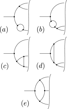
FIG. 16.: Ways to insert virtual subdiagrams in Feynman diagrams for $e^{+}e^{-}\to 3{\ \it partons}$.

This leaves virtual self-energy subgraphs. In case (a), there is a self energy subgraph on a propagator that enters the final state. This case requires a treatment different from that discussed in the previous sections. This is evident because there is a nominal $1/k^{2}$ where $k^{2}=0$. The treatment required is to represent the virtual self-energy via a dispersion relation [1]. In this representation, the subgraph is expressed as an integral over the three-momentum in the virtual loop with an integrand that is closely related to the integrand for the corresponding cut self-energy graph. The point-by-point cancellation between real and virtual graphs is then manifest. It is convenient also to use the dispersive representation for the much easier case (b).

Third, we have to do something about ultraviolet divergences in virtual subgraphs. These are easily removed [1] by subtracting an integrand that, in the region of large loop momenta, matches the integrand of the divergent subdiagram. The integrand of the subtraction term should depend on a mass parameter $\mu$ that serves to make the subtraction term well behaved in the infrared. Then, with the aid of a small analytical calculation for each of the one loop divergent subdiagrams that occur in QCD, one can arrange the definition so that this ad hoc subtraction has exactly the same effect as $\overline{\rm MS}$ subtraction with scale parameter $\mu$.

Fourth, I use Feynman gauge for the gluon field, but then self-energy corrections on a gluon propagator require special attention [1]. The one loop gluon self-energy subgraph, $\pi^{\mu\nu}(k)$, contains a term proportional to $k^{\mu}k^{\nu}$ that contributes quadratic infrared divergences [5], while the cancellation mechanism that we have studied in this paper takes care of logarithmic divergences. This problem can be solved by replacing $\pi^{\mu\nu}$ by $P^{\mu}_{\alpha}\pi^{\alpha\beta}P_{\beta}^{\nu}$, where $P^{\mu}_{\alpha}=g^{\mu}_{\alpha}-{k^{\mu}\tilde{k}_{\alpha}/\tilde{k}^{2}}$, with $\tilde{k}=(0,\vec{k})$. The terms added to $\pi^{\mu\nu}$ are proportional to either $k^{\mu}$ or $k^{\nu}$ and thus vanish when one sums over different ways of inserting the dressed gluon propagator into the remaining subgraph. Since $P^{\mu}_{\alpha}k^{\alpha}=0$, the problematic $k^{\mu}k^{\nu}$ term is eliminated. Effectively, this is a change of gauge for dressed gluon propagators from Feynman gauge to Coulomb gauge.

Most of these issues are discussed briefly in [1]. A quite detailed, but not very pedagogical, treatment can be found in [6]. Further analysis of these issues is left for a future paper.

I have also not given a complete presentation of algorithms for choosing integration points. As discussed in Sec. VI C, the crucial issue is to have the right singularities in the density of points near a soft parton singularity of the Feynman diagram. This is not the only issue that needs to be addressed in a complete algorithm. Of course, the demonstration program [3] has a complete algorithm. However, this algorithm is quite a hodge-podge of methods and it seems that a detailed exposition should be reserved for a better and more systematic method, which remains to be developed.

IX Results and conclusions

In the preceding sections, we have seen some of the techniques needed for the numerical integration method for QCD calculations. Of course, since not all of the techniques have been explained, the explanation does not constitute a very convincing argument that such a calculation is feasible. A truly exhaustive explanation would help, but an actual computer program that demonstrates the techniques is better. Results from such a program were presented in [1]. Since then, I have found and corrected one bug that resulted in errors a little bit bigger than 1% and have made some other improvements in the code. The resulting code and documentation are available at [3].

The program is a parton-level event generator. The user is to supply a subroutine that calculates how an event with three or four partons in the final state contributes to the observable to be calculated. The program supplies events, each consisting of a set of parton momenta $\{\vec{k}_{1},\vec{k}_{2},\vec{k}_{3}\}$ or $\{\vec{k}_{1},\vec{k}_{2},\vec{k}_{3},\vec{k}_{4}\}$, together with weights $w$ for the events. Then the user routine calculates ${\cal I}$ according to

$${\cal I}\approx{1\over N}\sum_{i=1}^{N}w_{i}\ {\cal S}(k_{i}).$$ (116)

The weights used are the real parts of complex weights; the imaginary parts can be dropped since we always know in advance that ${\cal I}$ is real. Thus the weights are both positive and negative. It would, of course, be more convenient to have only positive weights, but one can hardly have quantum interference without having negative numbers along with positive numbers.

The first general purpose program for QCD calculation of three-jet-like quantities in $e^{+}e^{-}\to{\it hadrons}$ at order $\alpha_{s}^{2}$ was that of Kunszt and Nason [7]. This program uses the numerical/analytical method of Ellis, Ross, and Terrano. In Table I, I compare the results of the Kunszt-Nason program to those obtained with the numerical method for the $\alpha_{s}^{2}$ contributions to moments of the thrust distribution,

$${\cal I}_{n}={1\over\sigma_{0}\,(\alpha_{s}/\pi)^{2}}\int_{0}^{1}\!dt\ (1-t)^{n}{d\sigma^{[2]}\over dt}.$$ (117)

In Table II, I compare the results of the two methods for moments of the $y_{\rm cut}$ distribution for the three jet cross section. To define these quantities, let $f_{3}(y_{\rm cut})$ be the cross section to produce three jets according to the Durham algorithm [8] with resolution parameter $y_{\rm cut}$. Let $g_{3}(y_{\rm cut})$ be the negative of its derivative,

$$g_{3}(y_{\rm cut})=-{f_{3}(y_{\rm cut})\over dy_{\rm cut}}.$$ (118)

Then we calculate moments of the $\alpha_{s}^{2}$ contribution to this quantity,

$${\cal I}_{n}={1\over\sigma_{0}\,(\alpha_{s}/\pi)^{2}}\int_{0}^{1}\!d\,y_{\rm cut}\ (y_{\rm cut})^{n}g_{3}^{[2]}.$$ (119)

In each table, the results for the numerical method are shown with their statistical and systematic errors. (The systematic error is estimated by changing the cutoffs that remove small regions near the singularities where roundoff errors start to become a problem.) The corresponding results for the numerical/analytical method are shown with the statistical errors as reported by the program. Inspection of the tables shows that there is good agreement between the two methods.

TABLE I.: Comparison of results for moments of the thrust distribution, Eq. (117). The “numerical” results are from the program [3]. The first error is statistical, the second systematic. The “numerical/analytical” results are from the program of Kunszt and Nason [7] and are given with their reported statistical errors.

n	numerical	numerical/analytical
1.5	$\hskip 3.80005pt4.127\pm 0.008\pm 0.025$	$\hskip 3.80005pt4.132\pm 0.003$
2.0	$\hskip 3.80005pt1.565\pm 0.002\pm 0.007$	$\hskip 3.80005pt1.565\pm 0.001$
2.5	$(6.439\pm 0.010\pm 0.022)\times 10^{-1}$	$(6.440\pm 0.003\hskip 5.0pt)\times 10^{-1}$
3.0	$(2.822\pm 0.005\pm 0.009)\times 10^{-1}$	$(2.822\pm 0.001\hskip 5.0pt)\times 10^{-1}$
3.5	$(1.296\pm 0.002\pm 0.004)\times 10^{-1}$	$(1.296\pm 0.0005)\times 10^{-1}$
4.0	$(6.159\pm 0.011\pm 0.016)\times 10^{-2}$	$(6.161\pm 0.002\hskip 5.0pt)\times 10^{-2}$
4.5	$(3.009\pm 0.006\pm 0.007)\times 10^{-2}$	$(3.010\pm 0.0006)\times 10^{-2}$
5.0	$(1.501\pm 0.003\pm 0.003)\times 10^{-2}$	$(1.502\pm 0.0002)\times 10^{-2}$

TABLE II.: Comparison of results for moments of the $y_{cut}$ distribution, Eq. (119). The “numerical” results are from the program [3]. The first error is statistical, the second systematic. The “numerical/analytical” results are from the program of Kunszt and Nason [7] and are given with their reported statistical errors.

n	numerical	numerical/analytical
1.5	$(8.442\pm 0.034\pm 0.059)\times 10^{-1}$	$(8.397\pm 0.002\hskip 5.0pt)\times 10^{-1}$
2.0	$(3.106\pm 0.012\pm 0.015)\times 10^{-1}$	$(3.090\pm 0.0004)\times 10^{-1}$
2.5	$(1.205\pm 0.005\pm 0.005)\times 10^{-1}$	$(1.200\pm 0.0002)\times 10^{-1}$
3.0	$(4.945\pm 0.025\pm 0.019)\times 10^{-2}$	$(4.927\pm 0.001\hskip 5.0pt)\times 10^{-2}$
3.5	$(2.122\pm 0.012\pm 0.008)\times 10^{-2}$	$(2.116\pm 0.0007)\times 10^{-2}$
4.0	$(9.430\pm 0.064\pm 0.032)\times 10^{-3}$	$(9.412\pm 0.004\hskip 5.0pt)\times 10^{-3}$
4.5	$(4.304\pm 0.034\pm 0.014)\times 10^{-3}$	$(4.301\pm 0.002\hskip 5.0pt)\times 10^{-3}$
5.0	$(2.008\pm 0.018\pm 0.006)\times 10^{-3}$	$(2.008\pm 0.001\hskip 5.0pt)\times 10^{-3}$

We have explored some of the most important techniques necessary for a QCD calculation for three-jet-like quantities in electron-positron annihilation at order $\alpha_{s}^{2}$ using numerical integration throughout the calculation. For the techniques covered, this explanation expands on the brief presentation in [1]. We have also seen that the method works. The older and very successful numerical/analytical method for QCD calculations has its complications. The numerical method has its own complications, but they are different complications. Thus one may expect that the classes of problems for which each of the methods is well adapted may be different. There may be some classes of problems for which the natural flexibility of the numerical method makes it the more useful method. It remains for the future to explore the possibilities.

Contour deformation in many dimensions

The calculational method described in this paper makes use of Cauchy’s theorem in a multi-dimensional complex space. Since this theorem is not proved in most textbooks on complex analysis, I provide a proof here, including the special case, needed for our application, in which there is a singularity on the integration contour.

Let $f(z)$ be a function of $N$ complex variables $z^{\mu}=x^{\mu}+iy^{\mu}$, with $\mu=1,\dots,N$, where $x^{\mu}$ and $y^{\mu}$ are real variables. Consider a family of integration contours ${\cal C}(t)$ labeled by a parameter $t$ with $0\leq t\leq 1$ and specified by

$$z^{\mu}(x^{1},\cdots,x^{N};t)=x^{\mu}+i\,y^{\mu}(x^{1},\cdots,x^{N};t),\hskip 56.9055pt\mu=1,\dots,N.$$ (120)

Let ${\cal I}(t)$ be the integral of $f$ over the contour ${\cal C}(t)$,

$${\cal I}(t)=\int_{{\cal C}(t)}\!d\,z\ f(z)=\int\!d\,x\ \det\!\left(\partial z(x;t)\over\partial x\right)\ f(z(x;t)).$$ (121)

Suppose that $f(z)$ is analytic in a region that contains the contours. Then we have Cauchy’s theorem:

$${\cal I}(1)={\cal I}(0).$$ (122)

To prove this theorem, we simply prove that $d\,{\cal I}(t)/d\,t=0$. Define

$$A^{\mu}_{\nu}={\partial z^{\mu}\over\partial x^{\nu}}=\delta^{\mu}_{\nu}+i\ {\partial y^{\mu}\over\partial x^{\nu}}.$$ (123)

Let $B^{\mu}_{\nu}$ be the inverse matrix to $A^{\mu}_{\nu}$. Then

$$B^{\mu}_{\nu}\det A={1\over(N-1)!}\epsilon^{\mu\mu_{2}\cdots\mu_{N}}\epsilon_{\nu\nu_{2}\cdots\nu_{N}}\,{\partial z^{\nu_{2}}\over\partial x^{\mu_{2}}}\cdots{\partial z^{\nu_{N}}\over\partial x^{\mu_{N}}},$$ (124)

where $\epsilon^{\mu_{1}\cdots\mu_{N}}$ is the completely antisymmetric tensor with $N$ indices, normalized to $\epsilon^{1\,2\cdots N}=1$, and $\epsilon_{\mu_{1}\cdots\mu_{N}}$ is the same tensor. This has the immediate consequence that

$${\partial\over\partial x^{\mu}}\,\left(B^{\mu}_{\nu}\det A\right)=0.$$ (125)

Also,

$$\det A={1\over N!}\ \epsilon^{\mu_{1}\cdots\mu_{N}}\epsilon_{\nu_{1}\cdots\nu_{N}}\,{\partial z^{\nu_{1}}\over\partial x^{\mu_{1}}}\cdots{\partial z^{\nu_{N}}\over\partial x^{\mu_{N}}},$$ (126)

so

$${\partial\over\partial t}\det A={\partial A^{\nu}_{\mu}\over\partial t}\ B^{\mu}_{\nu}\det A=i\,{\partial y^{\nu}\over\partial x^{\mu}\partial t}\ B^{\mu}_{\nu}\det A.$$ (127)

We need one more result:

$${\partial f\over\partial x^{\mu}}={\partial z^{\nu}\over\partial x^{\mu}}{\partial f\over\partial z^{\nu}},$$ (128)

so

$${\partial f\over\partial z^{\nu}}=B^{\mu}_{\nu}\ {\partial f\over\partial x^{\mu}}.$$ (129)

Then, using the results (125), (127), and (129) and an integration by parts, we find

$${d\over d\,t}\,{\cal I}(t) = \int\!d\,x\ {d\over d\,t}\,\left[\det A\ f\right]$$ (130)

$$= \int\!d\,x\ \det A\left\{i\,{\partial y^{\nu}\over\partial x^{\mu}\partial t}\ B^{\mu}_{\nu}\ f+{\partial f\over\partial z^{\nu}}\ i\,{\partial y^{\nu}\over\partial t}\right\}$$ (131)

$$= \int\!d\,x\ \det A\left\{i\,{\partial y^{\nu}\over\partial x^{\mu}\partial t}\ B^{\mu}_{\nu}\ f+i\,B^{\mu}_{\nu}\ {\partial f\over\partial x^{\mu}}\ {\partial y^{\nu}\over\partial t}\right\}$$ (132)

$$= i\int\!d\,x\ B^{\mu}_{\nu}\det A\ {\partial\over\partial x^{\mu}}\left\{{\partial y^{\nu}\over\partial t}\ f\right\}$$ (133)

$$= -i\int\!d\,x\ {\partial y^{\nu}\over\partial t}\ f\ {\partial\over\partial x^{\mu}}\left\{B^{\mu}_{\nu}\det A\right\}$$ (134)

$$= 0.$$ (135)

This proves the theorem.

Consider now a more complicated problem. Suppose that we have an integral of the form

$${\cal I}=\int\!d\,x\ [f(x)+g(x)].$$ (136)

where $f$ and $g$ are both singular on a surface ${\cal P}$ in the space of the real variables $x$. Suppose that the strength of the singularities are such that the integral of either function would be logarithmically divergent. Suppose further that there is a cancellation in the sum such that the integral of $f+g$ is convergent. Let $d(x)$ be the distance from any point $x$ to the surface ${\cal P}$. Let us cut out a region of radius $R$ around ${\cal P}$ and write

$${\cal I}=\lim_{R\to 0}\left[\int_{d>R}\!d\,x\ f(x)+\int_{d>R}\!d\,x\ g(x)\right].$$ (137)

Now we wish to explore the consequences of deforming the integration contour for the integral of $f$. Thus we investigate (with the same notation as above)

$${\cal I}(t)=\lim_{R\to 0}\left[\int_{d>R}\!d\,x\ \det\!\left(\partial z(x;t)\over\partial x\right)\ f(z(x;t))+\int_{d>R}\!d\,x\ g(x)\right].$$ (138)

Following the previous proof we find that there is a surface term in the integration by parts

$${d\over d\,t}\,{\cal I}(t) = \lim_{R\to 0}\left[i\int_{d<R}\!d\,x\ {\partial\over\partial x^{\mu}}\left\{B^{\mu}_{\nu}\det A\ {\partial y^{\nu}\over\partial t}\ f\right\}\right]$$ (139)

$$= \lim_{R\to 0}\left[i\int\!dS_{\mu}\left\{B^{\mu}_{\nu}\det A\ {\partial y^{\nu}\over\partial t}\ f\right\}\right],$$ (140)

where the integration is over the surface $d=R$ and $dS_{\mu}$ is the surface area differential normal to the surface.

We want to arrange the deformation specified by $y^{\mu}(x;t)$ so that $d{\cal I}(t)/dt=0$. For this to happen, it is clear that $y$ will have to approach 0 as $x$ approaches the surface ${\cal P}$. Then $B^{\mu}_{\nu}\to\delta^{\mu}_{\nu}$ and $\det A\to 1$ as $x$ approaches ${\cal P}$. Let the dimensionality of the singular surface ${\cal P}$ be $N-a$. If the function $f$ was such that the original integral was logarithmically divergent, then $f\propto R^{-a}$ for $R\to 0$. The integration over the surface gives a factor $dS^{\mu}\propto R^{a-1}$ for $R\to 0$. Suppose that the deformation vanishes proportionally to $R^{b}$. Then

$${d\over d\,t}\,{\cal I}(t)\propto\lim_{R\to 0}\left[R^{a-1}R^{a}R^{b}\right].$$ (141)

Then $d{\cal I}(t)/dt=0$ if $b>1$. The choice made in the main text of the paper is $b=2$.

REFERENCES

- [1] D. E. Soper, Phys. Rev. Lett. 81, 2638 (1998).
- [2] R. K. Ellis, D. A. Ross, and A. E. Terrano, Nucl. Phys. B178, 421 (1981).
- [3] D. E. Soper, beowulf Version 1.0, http://zebu.uoregon.edu/~soper/beowulf/.
- [4] Z. Kunszt and D. E. Soper, Phys. Rev. D 46, 192 (1992).
- [5] G. Sterman, Phys. Rev. D 17, 2773, 2789 (1978).
- [6] D. E. Soper, Beowulf 1.0 Technical Notes, http://zebu.uoregon.edu/~soper/beowulf/.
- [7] Z. Kunszt, P. Nason, G. Marchesini and B. R. Webber in Z Physics at LEP1, Vol. 1, edited by B. Altarelli, R. Kleiss ad C. Verzegnassi (CERN, Geneva, 1989), p. 373
- [8] Yu. L. Dokshitzer, contribution to the Workshop on Jets at LEP and HERA, Durham, December 1990; S. Bethke, Z. Kunszt, D. E. Soper and W. J. Stirling, Nucl. Phys. B370, 310 (1992), Erratum-ibid. B523, 681 (1998).