Jisuke Kubo, Haruhiko Terao and George Zoupanos

Institute for Theoretical Physics, Kanazawa University, Kanazawa 920-1192, Japan

Abstract

We present a method to control the regularization scheme dependence in the running of couplings in Kaluza-Klein theories. Specifically we consider the scalar theory in five dimensions, assuming that one dimension is compactified and we study various regularization schemes in order to analyze concretely the regularization scheme dependence of the Kaluza-Klein threshold effects. We find that in one-loop order, although the $\beta$-functions are different for the different schemes, the net difference in the running of the coupling among the different schemes is very small for the entire range of energies. Our results have been extended to include more than one radii, and the gauge coupling unification is re-examined. Strings are also used as a regulator. We obtain a particular regularization scheme of the effective field theory which can accurately describe the string Kaluza-Klein threshold effects.

PACS number: 11.10.Hi, 11.10.Kk, 11.25.Mj, 12.10.Kt
Keywords: Kaluza-Kein theory, Renormalization group, Gauge coupling unification

1 Introduction

Recently there have been renewed interests in Kaluza-Klein theories with a large compactification radius [2]–[6]. The radius can be so large that quantum effects, in particular the running of coupling constants in these theories, can drastically change the traditional picture of unification of the gauge couplings [5]. These higher dimensional field theories might appear as the low-energy effective theory of a string theory with certain $D$-branes [5]–[8] , and contain towers of massive Kaluza-Klein excitations. It is indeed this tower of excitations which gives rise to the quantum effect that modifies the behavior of the coupling from the logarithmic to the power law running [10, 5], thereby changing the usual unification scenario. The results of refs. [10, 5, 11, 12] indicate, moreover, that this quantum effect can be computed to a certain extent within the framework of the effective field theory . That is, physics below the string scale but above the compactification scale (the massive string states are suppressed in this regime), can be well described by a field theory [11, 12] which is unrenormalizable by power counting. Furthermore, it is expected that if extra dimensions are compactified the unrenormalizable theory effectively appears at low energies in four dimensions as a renormalizable theory, in which the massive Kaluza-Klein excitations are completely decoupled. How can this decoupling become possible in unrenormalizable theories? In this paper we are motivated by the desire to gain a deeper understanding on the Kaluza-Klein thresholds within the framework of (unrenormalizable) field theory.

A pragmatic way to define an unrenormalizable theory is to cutoff the high energy modes by a regularization. However, in contrast to renormalizable theories, it is no longer obvious that the “physical” quantities are truly independent of the regularization. Therefore, the regularization scheme dependence must be much more serious than the renormalization scheme dependence in renormalizable theories. To our knowledge there exists no complete solution to this problem. Our task in this paper is to take a step in solving this important problem in the case of the running of couplings. (Note that the running of couplings is strongly dependent on regularization.) To simplify the situation we will first consider the Kaluza-Klein theory for the scalar field with a self-interacting coupling in five dimensions where we assume that one extra dimension is compactified on a circle with radius $R$. We will assume that the leading high energy behavior in the running of the coupling is fixed by its canonical dimension without any corrections. From this we postulate in section 2 the form of the $\beta$-function of the dimensionally-reduced, four-dimensional theory containing the Kaluza-Klein tower and show that the regularization scheme dependence in the running of the coupling can be systematically controlled in the asymptotic regime (i.e. in energy scales much higher than the compactification scale $1/R$). In other words, different regularization schemes in the asymptotic regime can be related by a “finite” transformation of the corresponding coupling, in a very similar way as in the case of a renormalizable theory. Consequently, the net difference among regularization schemes can originate only from the threshold effect of the first Kaluza-Klein excitations.

In section 3 we will consider various regularization schemes, the Exact renormalization group (ERG) scheme [18]–[21] , the momentum subtraction scheme and the proper time regularization scheme [5], and we introduce the notion of effective dimension (which has been used to absorb the environmental effects at finite temperature into a redefinition of the spatial dimension [22]) to absorb the Kaluza-Klein threshold effects into the effective dimension. Studying the effective dimension as a function of energy, we will observe the smooth transition of the coupling from the logarithmic behavior to the power law behavior, which shows that the effective dimension contains the full information of the Kaluza-Klein threshold effects. In section 4 we will then investigate the one-loop evolution of the coupling in these schemes as well as in the one-$\theta$ function and the successive-$\theta$ functions approximation schemes, and extract the net difference among the schemes by taking into account appropriately chosen finite transformations of the coupling. We will find that the net difference in the evolution of the coupling among the different regularization schemes is very small. At first sight this looks like a surprising result, but in fact it only generalizes the result of ref. [5] that the one-$\theta$-function approximation is a very good approximation to the proper time regularization scheme. We expect that this feature of the threshold effect, which does not exist in the usual renormalizable theories, is very general in Kaluza-Klein theories, and therefore our result obtained in a scalar field theory can be extended to gauge theories. In fact we examine gauge coupling unification of the minimal supersymmetric standard model (MSSM) with the Kaluza-Klein tower only in the gauge and Higgs supermultiplets (proposed in ref. [5]) by taking into account the Kaluza-Klein threshold effect. We find that because of a compensating mechanism which exists in this model the prediction of $\alpha_{3}(M_{Z})$ does not change practically.

Finally we compare the Kaluza-Klein threshold effect in a string theory and its effective field theory. We will observe that string theory result averages those of field theory in different regularizations with a definite weight, and that it defines an average regularization scheme of the effective theory. Remarkably, we will find that the effective theory with the average regularization scheme can accurately describe the Kaluza-Klein threshold effects of the string theory.

2 Controlling regularization scheme dependence

In order to concentrate on the regularization scheme dependence and to avoid problems that might complicate our task (e.g. violation of gauge symmetries through regularization), we consider the Kaluza-Klein theory for the scalar field $\phi$ in Euclidean five dimensions where we assume that the one extra dimension is compactified on a circle with radius $R$. We denote the extra coordinate by $y$ and the four dimensional coordinates by $x_{\mu}$. The starting five dimensional action is

$$S^{(5)} = \int_{0}^{2\pi R}dy\int d^{4}x\left\{~{}\frac{1}{2}(\partial_{y}\tilde{\phi})^{2}+\frac{1}{2}(\partial_{\mu}\tilde{\phi})^{2}+\frac{\tilde{m}^{2}}{2}\tilde{\phi}^{2}+\frac{\tilde{\lambda}}{4!}\tilde{\phi}^{4}~{}\right\}~{}.$$ (1)

The scalar field satisfies the boundary condition

$$\tilde{\phi}(x,y) = \tilde{\phi}(x,y+2\pi R)~{},$$ (2)

which implies that the field can be expanded as

$$\tilde{\phi}(x,y) = \sum_{n\in{\bf Z}}~{}\tilde{\phi}_{n}(x)~{}\exp(i\omega_{n}y)~{},~{}~{}~{}~{}\omega_{n}=\frac{n}{R}~{},$$ (3)

$$(\tilde{\phi}_{n})^{*} = \tilde{\phi}_{-n}~{},$$

where the last equality follows from the reality of $\tilde{\phi}$. To define the four dimensional action we redefine the field and the parameters according to

$$\tilde{\phi}_{n} \to \phi_{n}=\tilde{\phi}_{n}/\sqrt{2\pi R}~{},~{}\tilde{\lambda}\to\lambda=2\pi R\tilde{\lambda}~{},~{}\tilde{m}^{2}\to m^{2}=\tilde{m}^{2}~{}.$$ (4)

We then obtain

$$S=\int d^{4}x\left\{\frac{1}{2}\sum_{n\in{\bf Z}}\phi_{-n}[-\partial_{\mu}^{2}+m^{2}+\omega_{n}^{2}]\phi_{n}+\frac{\lambda}{4!}\sum_{n_{i}\in{\bf Z}}\delta_{n_{1}+n_{2}+n_{3}+n_{4},0}\phi_{n_{1}}\phi_{n_{2}}\phi_{n_{3}}\phi_{n_{4}}\right\}.$$ (5)

The canonical dimension of the original coupling $\tilde{\lambda}$, defined in (1), is $-1$, and so one expects that $\tilde{\lambda}$ behaves like $\tilde{\lambda}\sim\Lambda^{-1}$ for large $\Lambda$. As we have announced in the introduction, we assume that the leading order behavior does not suffer from any scaling violation. This implies that the $\beta$-function of the coupling $\tilde{\lambda}$ in the five dimensional theory can be written as

$$\tilde{\beta} = \Lambda\frac{d\tilde{\lambda}}{d\Lambda}\simeq\sum_{n\geq 2}~{}\tilde{b}_{n}\tilde{\lambda}^{n}\Lambda^{n-1}~{}$$ (6)

for large $\Lambda$. In general it is expected that the expansion coefficients $\tilde{b}_{n}$ depend on the regularization scheme employed, even in the lowest order, i.e. $\tilde{b}_{2}$. Next if the four dimensional theory defined by (5) should be related or be an approximation to the five dimensional theory, then the $\beta$-function of $\lambda$ should approach, upon the rescaling (4), the form (6) of the five dimensional theory in the large $\Lambda$ limit. From this consideration we postulate that the $\beta$-function of $\lambda$ for large $\Lambda$ has the form

$$\beta=\Lambda\frac{d\lambda}{d\Lambda}=\sum_{n\geq 2}~{}b_{n}\lambda^{n}(R\Lambda)^{n-1}+\Delta\beta~{},$$ (7)

where $\Delta\beta$ stands for sub-leading terms which vanish in the $\Lambda\to\infty$ limit (with $\lambda$ kept constant). Like the coefficients $\tilde{b}_{n}$, the expansion coefficients $b_{n}$ depend on the regularization scheme.

Before we proceed, let us note the following remark. In usual renormalizable gauge theories, the renormalization scheme dependence has been systematically studied in ref. [30]. We recall that in this case there exists not only the complete parametrization of the renormalization scheme dependence, but also there exist exact, renormalization-scheme independent quantities at a given order in perturbation theory. It might be possible to generalize these results to non-renormalizable theories. However, the generalization will not be straightforward, because in renormalizable theories there exist quantities (i.e. the physical quantities) that are formally ensured to be independent of renormalization scheme if one considers all orders of the perturbative expansions.

Given the asymptotic form of the $\beta$-function (7) in four dimensions, we analyze the regularization dependence, and consider the change of the scheme, $\lambda\to\lambda^{\prime}$. We require that this transformation satisfies:

$$~{}\lambda^{\prime} \sim 1/\Lambda~{}~{}\mbox{as}~{}~{}\Lambda\to\infty~{}.$$ (8)

It is now straightforward to see that the most general form of the transformation that keeps the asymptotic form (7) invariant can be written as

$$\lambda \to \lambda^{\prime}=\sum_{n\geq 1}c_{n}\lambda^{n}(R\Lambda)^{n-1}+\Delta_{\lambda}~{},$$ (9)

where $c_{1}=1$, and $\Delta_{\lambda}$ stands for the terms in the sub-leading orders. It may be worthwhile to see how the transformation (9) changes the coefficients $b_{n}$ in lower orders.

To this end, we consider up to the next-to-leading order:

$$\beta = b_{2}\lambda^{2}(R\Lambda)+b_{3}\lambda^{3}(R\Lambda)^{2}+\dots~{},$$ (10)

$$\lambda^{\prime} = \lambda(1+c_{2}\lambda\Lambda+c_{3}\lambda\Lambda^{2}+\dots)~{},$$ (11)

and find that

$$\beta^{\prime} = \Lambda\frac{d\lambda^{\prime}}{d\Lambda}=b_{2}^{\prime}\lambda^{\prime 2}(R\Lambda)+b_{3}^{\prime}\lambda^{\prime 3}(R\Lambda)^{2}+\dots~{},$$ (12)

with $$b_{2}^{\prime}=b_{2}+c_{2}~{},~{}b_{3}^{\prime}=b_{3}-2c_{2}^{2}+2c_{3}~{}.$$ (13)

So the lowest order coefficient $b_{2}$ has been changed, which should be contrasted to the renormalizable case where the lowest order coefficient does not change under the change of scheme.

We will see that the discussion above plays an important role in the next section in taking into account the threshold corrections of the Kaluza-Klein modes and comparing the threshold effects obtained in different regularization schemes with each other.

3 Explicit calculations in different schemes

In order to describe the Kaluza-Klein threshold effects and obtain the power-law behavior of the effective couplings, it is important to treat the decoupling of the massive Kaluza-Klein modes faithfully. In this section we adopt three different regularization schemes of this kind; 1) the Exact RG (ERG) scheme (the Legendre flow equations) [21], 2) the momentum subtraction (MOM) scheme and 3) the proper time regularization (PT) scheme [5]. In what follows, we will study the regularization scheme dependence in the $\beta$-function and compare the results of these schemes.

3.1 Exact RG approach

A. Uncompactified case

The theory defined by (1) is (perturbatively) unrenormalizable by power-counting. Therefore we need to define the theory as a cutoff theory. The natural framework to study low-energy physics of the cutoff theory is provided by the continuous Wilson renormalization group (RG) [18]–[21]. To illustrate the basic idea of the Wilson RG approach, we assume for a while that the extra dimension is not compactified. First we divide the field in the momentum space, $\phi(p)$, into low and high energy modes according to

$$\phi(p)=\theta(|p|-\Lambda)\phi_{>}(p)+(1-\theta(|p|-\Lambda))\phi_{<}(p),$$ (14)

where $\theta(|p|-\Lambda)$ denotes a proper infrared cutoff function. The Wilsonian effective action is defined by integrating out the high energy modes in the path integral;

$$S_{\rm eff}[~{}\phi_{<},\Lambda~{}]=-\ln\left\{\int{\cal D}\phi_{>}~{}e^{-S[\phi_{>},\phi_{<}]}\right\}.$$ (15)

It was shown in ref. [18, 19] that the path integral corresponding to the difference

$$\delta S_{\rm eff}=S_{\rm eff}[~{}\phi_{<},\Lambda+\delta\Lambda~{}]-S_{\rm eff}[~{}\phi_{<},\Lambda~{}]$$ (16)

for an infinitesimal $\delta\Lambda$ can be exactly carried out. That is, it is possible to write down a concrete expression for the RG equation of the effective action in the form

$$\Lambda\frac{\partial S_{\rm eff}}{\partial\Lambda} = {\cal O}(S_{\rm eff})~{},$$ (17)

where ${\cal O}$ is a non-linear operator acting on the functional $S_{\rm eff}$. Since $S_{\rm eff}$ is a (non-local) functional of fields, one can think of the RG equation (17) as coupled differential equations for infinitely many couplings in the effective action. The crucial point is that ${\cal O}$ can be exactly derived for a given theory, in contrast to the perturbative RG approach where the RG equations are known only up to a certain order in perturbation theory. This provides us with possibilities to use approximation methods that go beyond the conventional perturbation theory [24, 25, 26].

There exist various (equivalent) formulations [19]–[21] of the ERG approach, and depending on the formulation and also on the cutoff scheme one has to consider different forms of the operator ${\cal O}$ . Of the different formulations, the so-called Legendre flow equation [21] is the most suitable one to incorporate the decoupling of heavy particles . Here let us first briefly outline the basic idea to derive the Legendre flow equation that describes the evolution of the cutoff effective action. As a first step we define the generating functional $W[J]$ of the connected Green’s functions with an infrared cutoff $\Lambda$ by

$$W[J]=\ln\int{\cal D}\phi\,\exp\left\{~{}\int\frac{d^{D}p}{(2\pi)^{D}}\,[\,-\frac{1}{2}\phi(-p)C^{-1}(p,\Lambda)\phi(p)]-S_{\Lambda_{0}}[\phi]+\phi\cdot J~{}\right\}~{},$$ (18)

where $D=5$ in the present case, and

$$\phi\cdot J~{}=~{}\int\frac{d^{D}p}{(2\pi)^{D}}~{}J(-p)\phi(p)~{}.$$ (19)

Here $S_{\Lambda_{0}}$ stands for the bare action, and $C^{-1}(p,\Lambda)$ is a smooth cutoff function of $p^{2}$ and $\Lambda^{2}$ which cutoffs the propagation of the lower energy modes with $|p|\ll\Lambda$. The explicit form of the cutoff function will be specified later on. An ultraviolet cutoff is assumed in the r.h.side of (18), but the results we will obtain are ultraviolet finite. One derives the RG equation for $W[J]$ for the present system by differentiating the both sides of eq. (18) with respect to $\Lambda$:

$$\Lambda\frac{\partial W}{\partial\Lambda} = -\frac{1}{2}\int\frac{d^{D}p}{(2\pi)^{D}}\,\left[~{}\frac{\delta W}{\delta J(p)}\,(\Lambda\frac{\partial C^{-1}(p,\Lambda)}{\partial\Lambda})\,\frac{\delta W}{\delta J(-p)}\right.$$ (20)

$$+\left.(\Lambda\frac{\partial C^{-1}(p,\Lambda)}{\partial\Lambda})\,\frac{\delta^{2}W}{\delta J(p)\delta J(-p)}\,\right]~{}.$$

This flow equation can be translated to that of the infrared cutoff effective action which is defined by Legendre transformation:

$$\Gamma_{\rm eff}[\phi] = -W[J]+J\cdot\phi-\frac{1}{2}\int\frac{d^{D}p}{(2\pi)^{D}}\,\phi(-p)C^{-1}(p,\Lambda)\phi(p)~{},$$ (21)

yielding

$$\Lambda\frac{\partial\Gamma_{\rm eff}}{\partial\Lambda}=\frac{1}{2}\,\int\frac{d^{D}p}{(2\pi)^{D}}\,\Lambda\frac{\partial C^{-1}(p,\Lambda)}{\partial\Lambda}~{}\left[~{}C^{-1}(p,\Lambda)+\frac{\delta^{2}\Gamma_{\rm eff}}{\delta\phi(p)\delta\phi(-p)}~{}\right]^{-1}~{}.$$ (22)

As we see from the above RG equations (20) and (22), they explicitly depend on the cutoff function $C(p,\Lambda)$. The physical quantities should be independent of it. However, this is not automatically ensured as we have emphasized in section 1. In this paper we use the smooth cutoff function

$$C(p,\Lambda)=\frac{1}{\Lambda^{2}}~{}\left(\frac{p^{2}}{\Lambda^{2}}\right)^{k}~{},$$ (23)

where $k$ is a positive integer satisfying $k>D/2-2$. To see that this is in fact an infrared cutoff, we look at the (massless) propagator which can be read off from the generating function (18):

$$\frac{1}{p^{2}}\theta_{\Lambda}(p^{2}/\Lambda^{2})~{}~{}~{}\mbox{with}~{}~{}\theta_{\Lambda}(s)=\frac{s^{k+1}}{1+s^{k+1}}~{}.$$ (24)

One sees that the cutoff profile becomes sharper for bigger $k$. (Later we will examine the cases of $k=1$ (slow cutoff) and $k=5$ (sharp cutoff) .) For the cutoff function (23) the ERG equation (22) becomes finally

$$\Lambda\frac{\partial\Gamma_{\rm eff}}{\partial\Lambda} = (k+1)\,\int\frac{d^{D}p}{(2\pi)^{D}}\,\left[~{}1+\frac{1}{\Lambda^{2}}~{}(\frac{p^{2}}{\Lambda^{2}})^{k}~{}\frac{\delta^{2}\Gamma_{\rm eff}}{\delta\phi(p)\delta\phi(-p)}~{}\right]^{-1}~{}.$$ (25)

The RG equations (22) and (25) are integro-differential equations of first order in $\Lambda$ defined on a space of functionals of fields. In general, these RG equations cannot be solved exactly, and therefore one has to apply some approximation method. Clearly, assumptions which are made for a specific approximation method should be confirmed in a case-by-case analysis at a desired level within the approximation scheme. In the derivative expansion approximation [24, 25], one assumes that the Legendre effective action $\Gamma_{\rm eff}[\phi]$ can be written as a space-time integral of a (quasi) local function of $\phi$, i.e.,

$$\Gamma_{\rm eff}[\phi] = \int d^{D}x\,(\,\frac{1}{2}\,\partial_{\mu}\phi\partial_{\mu}\phi\,Z_{\phi}(\phi)+V(\phi,\Lambda)+\dots~{})~{},$$ (26)

where $\dots$ stands for terms with higher order derivatives with respect to the space-time coordinates. In the lowest order of the derivative expansion (the local potential approximation (LPA) [23]), there is no wave function renormalization ($Z_{\phi}(\phi)=1$) and the RG equation for the effective potential $V$ can be obtained. It is more convenient to work with the RG equation for dimensionless quantities, which makes the scaling properties more transparent. To this end, we scale the quantities according to

$$p \to\Lambda p~{},~{}\phi\to\Lambda^{D/2-1}\phi~{},~{}V\to\Lambda^{D}V~{}.$$ (27)

Then the RG equation is found to be

$$\Lambda\frac{\partial V}{\partial\Lambda} = -DV+\frac{D-2}{2}\phi V^{\prime}+(k+1)\frac{A_{D}}{2}\int_{0}^{\infty}ds\,s^{D/2-1}\,\left[~{}1+s^{k}(s+V^{\prime\prime})~{}\right]^{-1}~{},$$ (28)

where the prime on $V$ stands for the derivative with respect to $\phi$, and

$$A_{D} = \frac{2^{1-D}}{\pi^{D/2}\Gamma(D/2)}$$ (29)

is the $D$ dimensional angular integral.

Since we are not interested in the non-perturbative calculations, but in the threshold effects of the Kaluza-Klein modes in the weak coupling regime, we assume that the potential $V$ in eq. (28) can be expanded as

$$V = \frac{1}{2}m^{2}\phi^{2}+\frac{1}{4!}\lambda\phi^{4}+\dots~{}.$$ (30)

This gives the RG equations for the effective couplings;

$$\Lambda\frac{\partial m^{2}}{\partial\Lambda} = -2m^{2}-\lambda(k+1)\frac{A_{D}}{2}\int_{0}^{\infty}dss^{D/2-1}\frac{s^{k}}{(1+s^{k+1}+m^{2}s^{k})^{2}}~{},$$ (31)

$$\Lambda\frac{\partial\lambda}{\partial\Lambda} = (D-4)\lambda+6\lambda^{2}(k+1)\frac{A_{D}}{2}\int_{0}^{\infty}dss^{D/2-1}\frac{s^{2}k}{(1+s^{k+1}+m^{2}s^{k})^{3}}~{}.$$ (32)

It is worth-considering the massless case, because $m^{2}$ (which is the mass of the zero mode in Kaluza-Klein theories) is small as compared to the scale of compactification in most practical situations. Then we find that

$$\Lambda\frac{\partial\lambda}{\partial\Lambda} = (D-4)\lambda+\frac{3}{2}A_{D}B(D,k)\lambda^{2}~{},$$ (33)

$$B(D,k) = 2(k+1)\int_{0}^{\infty}dss^{D/2-1}\frac{s^{2k}}{(1+s^{k+1})^{3}}~{}.$$ (34)

In terms of the original, dimensional coupling (i.e. $\lambda\to\Lambda^{D-4}\lambda$), the evolution equation (33) becomes

$$\Lambda\frac{\partial\lambda}{\partial\Lambda} = \frac{3}{2}A_{D}B(D,k)\Lambda^{4-D}\lambda^{2}~{},$$ (35)

recovering the power law behavior of the scalar coupling. Note that the constant $B(D,k)$ depends explicitly on $k$ and $D$ ($k>D/2-2$). We find, for instance, that

$$B(4,k)=1~{}~{}~{}\mbox{(for all $k$)},$$

$$B(5,1)=1.3884\cdots,~{}~{}~{}B(5,2)=1.22173\dots,~{}~{}~{}B(5,5)=1.09581\dots~{},$$

$$B(6,5)=1.22173\cdots~{}.$$ (36)

As we can see from eq. (35), the $k$ dependence (regularization dependence) can be absorbed into the redefinition of the coupling $\lambda$ for $D\neq 4$, according to the discussion of section 2. Fortunately, at $D=4$ (where the power behavior disappears) the $k$ dependence vanishes, as we see from (36).

B. Compactified case

Now we would like to come to the case in which the extra spatial dimension is compactified on a circle with radius $R$. What follows is a continuation of ref. [15] and a justification of the main assumptions that have been made there. The results of ref. [15] were also based on the recent developments that have been made concerning the renormalization properties of the supersymmetry breaking parameters in supersymmetric gauge theories [29].

The starting four dimensional action is given by eq. (5). To define the generating functional $W[J]$, we introduce like eq. (18) the infrared cutoff term

$$\Delta S = \frac{1}{2}\int_{0}^{2\pi R}dy\int d^{4}x\phi(x,y)C^{-1}(-i\partial_{x},-i\partial_{y},\Lambda)\phi(x,y)$$ (37)

$$= \frac{1}{2}\int\frac{dp^{4}}{(2\pi)^{4}}\sum_{n}\phi_{-n}(-p)C^{-1}(p,\omega_{n},\Lambda)\phi_{n}(p)~{}.$$

Then we follow exactly the same procedure as in the uncompactified case, and obtain the RG equation for the effective action:

$$\Lambda\frac{\partial\Gamma_{\rm eff}}{\partial\Lambda} = (k+1)\,\int\frac{d^{4}p}{(2\pi)^{4}}\,\sum_{n}~{}\Delta_{n,-n}(p,-p)~{},$$ (38)

$$\Delta^{-1}_{n,-m}(p,-p) = \delta_{n,-m}+\frac{1}{\Lambda^{2}}~{}(\frac{p^{2}+\omega_{n}^{2}}{\Lambda^{2}})^{k}~{}\frac{\delta^{2}\Gamma_{\rm eff}}{\delta\phi_{n}(p)\delta\phi_{-m}(-p)}~{},$$ (39)

where we have used the infrared cutoff function

$$C(p,\omega_{n},\Lambda) = \frac{1}{\Lambda^{2}}[~{}\frac{p^{2}+\omega_{n}^{2}}{\Lambda^{2}}~{}]^{k}~{}.$$ (40)

This infrared cutoff function is motivated from that of the uncompactified case (see eq. (23)). Calculating the propagator for a Kaluza-Klein mode, we find that it is multiplied by the cutoff function

$$\theta_{\Lambda}(p,\omega_{n}) = \frac{[~{}p^{2}/\Lambda^{2}+(\omega_{n}/\Lambda)^{2}~{}]^{k+1}}{1+[~{}p^{2}/\Lambda^{2}+(\omega_{n}/\Lambda)^{2}~{}]^{k+1}}~{},$$ (41)

from which we see that not only high frequency modes are integrated out in the effective action, but also heavy mass modes.

We keep following the uncompactified case. In the lowest order of the derivative expansion approximation the Legendre effective action $\Gamma_{\rm eff}[\phi]$ has the same form as (26), i.e.,

$$\Gamma_{\rm eff}[\phi_{n}] = \int d^{4}x\,\left(\,\frac{1}{2}\,\sum_{n}\partial_{\mu}\phi_{n}\partial_{\mu}\phi_{-n}+V(\phi_{n},\Lambda)+\dots~{}\right)~{},$$ (42)

and the potential has the same structure as the tree level

$$V=\frac{m^{2}}{2}\sum_{n}\phi_{-n}\left[-\partial_{\mu}^{2}+m^{2}+\omega_{n}^{2}~{}\right]\phi_{n}+\frac{\lambda}{4!}\sum_{n_{i}}\delta_{n_{1}+n_{2}+n_{3}+n_{4},0}\phi_{n_{1}}\phi_{n_{2}}\phi_{n_{3}}\phi_{n_{4}}+\dots~{}.$$ (43)

Then we scale the quantities according to (27) and inserting the ansatz (42) with $V$ given in eq. (43) into eq. (38) to obtain

$$\Lambda\frac{\partial V}{\partial\Lambda} = -4V+\sum_{n}\phi_{n}\frac{\partial V}{\partial\phi_{n}}$$ (44)

$$+(k+1)\frac{A_{4}}{2}\sum_{n}\int_{0}^{\infty}ds\,s^{4/2-1}\,\left[~{}1+s^{k}\left(s+\frac{\delta^{2}V}{\delta\phi_{n}(p)\delta\phi_{-n}(-p)}\right)~{}\right]^{-1}~{}.$$

Expanding the potential in eq. (44) we finally obtain the RG equations in one-loop approximation as

$$\Lambda\frac{\partial m^{2}}{\partial\Lambda} = -2m^{2}-\lambda(k+1)\sum_{n}~{}\frac{1}{16\pi^{2}}\int_{0}^{\infty}dss\frac{s_{n}^{k}}{(1+s_{n}^{k+1}+m^{2}s^{k})^{2}}~{},$$ (45)

$$\Lambda\frac{\partial\lambda}{\partial\Lambda} = 6\lambda^{2}(k+1)\sum_{n}~{}\frac{1}{16\pi^{2}}\int_{0}^{\infty}dss\frac{s_{n}^{2k}}{(1+s_{n}^{k+1}+m^{2}s^{k})^{3}}~{},$$ (46)

where

$$s_{n} = s+(\frac{n}{R\Lambda})^{2}~{}~{}\mbox{and}~{}~{}~{}\frac{A_{4}}{2}=\frac{1}{16\pi^{2}}~{}.$$ (47)

These RG equations should be compared with eqs. (31) and (32) found in the uncompactified case. Note that the sum over $n$ is convergent, and this convergence is ensured by the infrared cutoff function $C$ given in eq. (40) introduced in eq. (37).

3.2 Effective dimension

Here we would like to understand how the power behavior of the coupling for large $\Lambda$ occurs in the ERG scheme. To simplify things we consider the massless case. The evolution equation (46) in the massless limit becomes

$$\Lambda\frac{d\lambda}{d\Lambda}=\frac{3}{16\pi^{2}}~{}\epsilon_{k}(R\Lambda)~{}\lambda^{2}~{},$$ (48)

where

$$\epsilon_{k}(R\Lambda)=2(k+1)\sum_{n}~{}\int_{0}^{\infty}dss\frac{s_{n}^{2k}}{(1+s_{n}^{k+1})^{3}}~{},~{}s_{n}=s+\left(\frac{n}{R\Lambda}\right)^{2}~{}.$$ (49)

The function $\epsilon_{k}(R\Lambda)$ approaches to $1$ as $R\Lambda\to 0$, (i.e. $\Lambda\to 0$), while as $R\Lambda\to\infty$ its derivative, $d\ln\epsilon_{k}/d\ln\Lambda$, approaches to a constant independent of $\Lambda$. In figs. 1 and 2 we plot $\ln\epsilon_{k}$ as a function of $t=\ln(R\Lambda)$ for $k=1$ and $5$, respectively, where $N$ stands for the value of $n$ in the r.h.side of eq. (49) at which the sum is truncated (i.e. $|n|\leq N$).

Figure 1: The function $\ln\epsilon_{k}(t)$ with $k=1$ where $t=\ln(R\Lambda)$. $N$ stands for the cutoff in the sum over the Kaluza-Klein excitations.

Figure 2: The same as the fig. 1 with $k=5$.

The asymptotic behavior of the $\beta$-function can be read off from figs. 1 and 2, and we see that it agrees with the expectation presented in (7). In the present case, the $\beta$-function obeys the power law behavior starting around $(R\Lambda)\sim 1$ (i.e. $t\sim 0$). As we can see from figs. 1 and 2 the function $\epsilon_{k}(t)$ interpolates the two regions of energy, below and above the compactification scale $1/R$. In fact, we may regard

$$D_{\rm eff}(R\Lambda)=4+\frac{d\ln\epsilon_{k}}{d\ln(R\Lambda)}$$ (50)

as the effective dimension , because the redefined coupling by

$$h_{k} = ~{}\epsilon_{k}(R\Lambda)\lambda~{}$$ (51)

satisfies the RG equation ;

$$\Lambda\frac{dh_{k}}{d\Lambda} = (D_{\rm eff}-4)h_{k}+\frac{3}{16\pi^{2}}~{}h_{k}^{2}~{}.$$ (52)

One indeed finds that

$$D_{\rm eff}(R\Lambda)~{}\to~{}\left\{\begin{array}[]{c}4\\ 5\end{array}\right.~{}~{}\mbox{ as}~{}~{}R\Lambda~{}\to~{}\left\{\begin{array}[]{c}0\\ \infty\end{array}\right.~{}.$$ (57)

This is demonstrated in figs. 3 and 4 with $k=1$ and $5$, respectively (where the sum in eq. (49) is truncated at $N$).

Figure 3: The effective dimension $D_{\rm eff}(R\Lambda)$ for $k=1$ where $t=\ln(R\Lambda)$.

Figure 4: The same as fig. 3 with $k=5$.

At this point we emphasize that the function $\epsilon_{k}$ contains the full information of the threshold effects of the Kaluza-Klein excitations. That is, the solution of the evolution eq. (48) contains all the threshold effects.

Another important point is that the behavior of the effective dimension $D_{\rm eff}$ (which contains the infinite sum over the Kaluza-Klein excitations, see eq. (49)) near the compactification scale $1/R$ (in which the power law behavior of the coupling is not yet manifest) can be well approximated by the sum over only the first few Kaluza-Klein excitations. We see from figs. 2, 3 and 4 that only the first few Kaluza-Klein excitations give important contributions to the threshold effects. That is, it is not necessary to carry out the infinite sum in order to find the form of the correction coming from the Kaluza-Klein threshold effects. The coupling has the power law behavior already after passing few Kaluza-Klein excitations, and consequently, the $\beta$-function has reached its asymptotic form given in eq. (7). That is, the Kaluza-Klein excitations should be indeed present for the coupling to obey the power law, but the asymptotic behavior, i.e. $b_{2}$ given in (7), can be fixed through the first few excitations.

As a last task of this subsection we explicitly calculate the asymptotic form of the $\beta$-function for two different $k$’s, where $k$ specifies the cutoff function $C$ given in eq. (40) in the ERG scheme. We find

$$(16\pi^{2})b_{2}=\left\{\begin{array}[]{l}5.5536\cdots\\ 4.3832\cdots\end{array}\right.~{}~{}\mbox{for}~{}~{}k=\left\{\begin{array}[]{l}1\\ 5\end{array}\right.~{},$$ (62)

where the asymptotic coefficient $b_{2}$ is defined in eq. (7).

3.3 Momentum subtraction scheme

Here we analyze the momentum subtraction (MOM) scheme . To this end, we compute in the MOM scheme the one-loop correction $\Pi^{(4)}_{\rm MOM}$ to the four point vertex function in the four dimensional theory defined by the action in eq. (5). We find that for the massless case

$$\Pi^{(4)}_{\rm MOM}(q^{2},\Lambda^{2}=Q^{2},m_{n}^{2})$$ (63)

$$= \frac{3}{2}~{}\lambda^{2}~{}\int\frac{d^{4}p}{(2\pi)^{4}}~{}\sum_{n}~{}\left[~{}\frac{1}{(p^{2}+m_{n}^{2})((p-q)^{2}+m_{n}^{2})}-(q\to Q)~{}\right]~{},$$

from which we obtain the one-loop $\beta$-function in the MOM scheme;

$$\beta_{\rm MOM}=\Lambda\frac{\partial\Pi_{\rm MOM}}{\partial\Lambda}=\frac{3}{16\pi^{2}}\epsilon_{\rm MOM}(R\Lambda)~{}\lambda^{2},$$ (64)

where

$$\epsilon_{\rm MOM}(R\Lambda)=1+\sum_{n\neq 0}\int_{0}^{1}dx\frac{x(1-x)(R\Lambda/n)^{2}}{1+x(1-x)(R\Lambda/n)^{2}}~{}.$$ (65)

As we did in the case of the ERG scheme (see eq. (51)), we introduce the effective dimension in the MOM scheme:

$$D_{\rm eff}=4+\frac{d\ln\epsilon_{\rm MOM}}{d\ln(R\Lambda)}~{}.$$ (66)

In figs. 5 and 6 we plot $\ln\epsilon_{\rm MOM}$ and the $D_{\rm eff}$ in the MOM scheme as a function of $t=\ln(R\Lambda)$.

Figure 5: $\ln\epsilon_{\rm MOM}$ as a function of $t=\ln(R\Lambda)$.

Figure 6: The effective dimension $D_{\rm eff}$ as a function of $t=\ln(R\Lambda)$.

We see from figs. 5 and 6 that the power law behavior of the $\beta$-function in the MOM scheme can take place for $R\Lambda\sim 2$ (i.e. $t\sim 0.7$). The asymptotic form in the MOM scheme is found to be:

$$16\pi^{2}b_{2}=3.0701\cdots~{}.$$ (67)

However, in contrast to the non-perturbative RG approach, the transition region (i.e. $t\sim 0$) cannot be approximated by the sum over only the first few excitations; we need to sum over $\sim 40$ excitations, as is demonstrated in fig. 6. Therefore, we can conclude that the MOM scheme is not an economical one from this point of view.

3.4 Proper time scheme

Next we consider the proper time (PT) scheme. This is the approximation used in refs. [10, 5]. So following them, we compute as in the MOM scheme the one-loop correction $\Pi^{(4)}$ to the four point vertex function with zero external momenta in the PT scheme, and find

$$\Pi^{(4)}_{{\rm PT},(r)} = \frac{3}{2}~{}\lambda^{2}~{}\int^{\prime}\frac{d^{4}p}{(2\pi)^{4}}~{}\sum_{n}\frac{1}{(p^{2}+m_{n}^{2})^{2}}\$$ (68)

$$= \frac{\lambda^{2}}{8\pi^{2}}\frac{3}{2}\int^{\mu^{-2}}_{r\Lambda^{-2}}\frac{dt}{t}~{}\left(\frac{1}{2}\right)~{}~{}\vartheta_{3}\left(\frac{it}{\pi R^{2}}\right)~{},$$ (69)

where $\vartheta_{3}$ is one of the Jacobi theta functions

$$\vartheta_{3}(\tau) = \sum_{n=-\infty}^{\infty}\exp(i\pi n^{2}\tau)~{},$$ (70)

and $\prime$ means that the $p$ integral is cutoff. Note that an ultraviolet and infrared cutoff (by scale $\mu$) are introduced to make the $t$ integral finite, though the beta function is independent of the infrared cutoff. We emphasize that the factor $r$ cannot be fixed within the framework of the four dimensional theory, and so it is an ambiguity that belongs to the regularization scheme dependence uncertainties. In ref. [5] a specific value was given;

$$r = \pi(X_{\delta})^{-2/\delta}~{},~{}X_{\delta}=\frac{\pi^{\delta/2}}{\Gamma(1+\delta/2)}~{},$$ (71)

which has been obtained by comparing the asymptotic formula of $\vartheta_{3}$ (given in eq. (70)) and the total number of the Kaluza-Klein states with masses squared smaller than $\Lambda^{2}$. In the case at hand ($\delta=1$) we have $r=\pi/4$. But the difference between $r=\pi/4$ and another value can be completely transformed away by means of the lowest non-trivial order transformation given in eq. (9), as we have explicitly verified .

The $\beta$-function in the PT scheme is then

$$\beta_{{\rm PT},(r)}=\Lambda\frac{\partial\Pi_{{\rm PT},(r)}}{\partial\Lambda}=\frac{3}{16\pi^{2}}\epsilon_{{\rm PT},(r)}(R\Lambda)~{}\lambda^{2}~{},$$ (72)

where

$$\epsilon_{{\rm PT},(r)}(R\Lambda)=\vartheta_{3}\left(\frac{ir}{\pi(R\Lambda)^{2}}\right)=1+\sum_{n\neq 0}\exp\left(-\frac{rn^{2}}{(R\Lambda)^{2}}\right)~{}.$$ (73)

In fig. 7 and 8 we plot, respectively, $\ln\epsilon_{\rm PT,r}$ and the effective dimension

$$D_{\rm eff}(R\Lambda)=4+\frac{d\ln\epsilon_{{\rm PT},(r)}(R\Lambda)}{d\ln(R\Lambda)}$$ (74)

as a function of $t=\ln(R\Lambda)$. for $r=\pi/4$.

We see from figs.7 and 8 that the power law behavior of the coupling in the PT scheme can become manifest even before $R\Lambda\sim 1$ (i.e. $t\sim 0$). Moreover, the threshold region (i.e. $R\Lambda\sim 1$) can be very well approximated by the sum over the first few excitations, which is shown in fig. 8.

Figure 7: $\ln\epsilon_{\rm PT}$ with $r=\pi/4$ as a function of $t=\ln(R\Lambda)$ in the PT scheme.

Figure 8: The effective dimension $D_{\rm eff}$ as a function of $t=\ln(R\Lambda)$ for the PT scheme.

The asymptotic form in the PT scheme (with $r=\pi/4$) turns out be

$$16\pi^{2}b_{2}=6$$ (75)

where $b_{2}$ is defined in eq. (7).

3.5 Two dimensional torus compactification

The investigation performed so far may be extended to the case with compactified dimensions more than one. (The ERG scheme and the proper time scheme are applicable for any dimensions. However, as for the momentum subtraction scheme defined by eq. (63), the infinite sum of the Kaluza-Klein modes diverges for more than one compactified dimensions.) Here we will examine the behavior of the effective dimensions in the $D=6$ case of the torus compactification with two hierarchically different radii $R_{1}$ and $R_{2}$ $(R_{1}\ll R_{2})$. The asymptotic behavior of the RG equation at high energy scale $\Lambda$ will be given by

$$\Lambda\frac{\partial\lambda}{\partial\Lambda}\sim b_{2}\Lambda^{-2}\lambda^{2}+\cdots,$$ (76)

and the effective dimensionality will be $6$ in the present case. However, it is expected that the effective dimension is $5$ at the intermediate scale of $R_{1}\ll\Lambda\ll R_{2}$, and that successive dimensional crossover, $D_{\mbox{eff}}=6\to 5\to 4$, occurs as the Kaluza-Klein modes decouple successively.

Extension of the formulae for the $\beta$-function coefficients given by eq. (49) in the ERG scheme and by eq. (73) in the PT scheme to the $D=6$ case is straightforward; in the ERG scheme

$$\epsilon_{k}(R_{1}\Lambda,R_{2}\Lambda) = 2(k+1)\sum_{n_{1}}\sum_{n_{2}}\int_{0}^{\infty}dss\frac{s_{n_{1},n_{2}}^{2k}}{(1+s_{n_{1},n_{2}}^{k+1})^{3}},$$

$$s_{n_{1},n_{2}} = s+\left(\frac{n_{1}}{R_{1}\Lambda}\right)^{2}+\left(\frac{n_{2}}{R_{2}\Lambda}\right)^{2},$$ (77)

and in the PT scheme

$$\epsilon_{\mbox{PT},(r)}(R_{1}\Lambda,R_{2}\Lambda) = \sum_{n_{1}}\sum_{n_{2}}\exp\left(-r\left[\left(\frac{n_{1}}{R_{1}\Lambda}\right)^{2}+\left(\frac{n_{2}}{R_{2}\Lambda}\right)^{2}\right]\right)~{}$$ (78)

$$= \vartheta_{3}\left(\frac{ir}{\pi(R_{1}\Lambda)^{2}}\right)~{}\vartheta_{3}\left(\frac{ir}{\pi(R_{2}\Lambda)^{2}}\right)~{}.$$

The prescription of ref. [5] gives $r=1$ in this case. The effective dimension may be also defined from these functions as

$$D_{\mbox{eff}}(R_{1}\Lambda)=4+\frac{d\ln\epsilon_{i}(R_{1}\Lambda,R_{2}/R_{1})}{d\ln(R_{1}\Lambda)}.$$ (79)

In fig. 9 the effective dimension $D_{\mbox{eff}}$ as a function of $t=\ln(R_{1}\Lambda)$ in the torus compactification is shown, where the radius ratio of the torus is set equal to $R_{2}/R_{1}=10$. Results are obtained for $k=5$ in the ERG scheme and $r=1$ in the PT scheme.

Figure 9: The effective dimension $D_{\mbox{eff}}$ as a function of $t=\ln(R_{1}\Lambda)$ in the case that the compactified dimension is a torus with radius ratio of $R_{2}/R_{1}=10$. Results in the ERG scheme $(k=5)$ and in the PT scheme are shown.

The successive dimensional crossover is presented in fig. 9. It is noted that the PT scheme gives a smooth transition of the effective dimensionality.

4 Results and applications

4.1 Comparison

We have explicitly seen in the previous section that all the regularization schemes we have considered belong to the equivalent class of the schemes in which the asymptotic limit of the coupling obeys the same power law. This is the basis which enables us to make a meaningful comparison of the results obtained in the different schemes. Since we stay within the one-loop approximation, we may assume that the coupling constant $\lambda$ in all the schemes has the same value, say $\lambda_{0}$, at $\Lambda_{0}$ which is very much smaller than $1/R$. Furthermore, for $\Lambda$ much below $1/R$, all the schemes have the same one-loop $\beta$-function, and the difference among the different schemes must become larger and larger when closing to the transition region. After the transition region the difference of the schemes can be well controlled, and the result obtained in one scheme can be transformed into the equivalent one in such a way that they can be meaningfully compared.

To proceed, we define a scheme which has no threshold correction (the one-$\theta$ function approximation):

$$\beta_{0} = \frac{1}{16\pi^{2}}\lambda^{2}~{}[~{}3\theta(1-R\Lambda)+6\theta(R\Lambda-1)(R\Lambda)~{}]~{},$$ (80)

where we have used as the coefficient for the second term the one suggested in ref. [5]. That is, the scheme is specified by

$$(16\pi^{2})b_{2} = 6~{}.$$ (81)

We would like to transform the result obtained, say in the $i$-scheme specified by $16\pi^{2}b_{2i}$, to a reference scheme for which we choose the PT scheme which is specified by $16\pi^{2}b_{2}=6$ as in the case of the one-$\theta$ function scheme. According to eq. (9), the transformation has the form

$$\lambda_{i}~{}\to~{}\lambda_{i}+c_{2i}\lambda^{2}\Lambda~{}.$$ (82)

The subscript $i$ should indicate that the actual values of the transformed $\lambda_{i}$ differ from one scheme to another, although all the schemes have been brought into the same scheme through the transformation (82) upon using eqs. (13). This difference will be the net difference of the regularization schemes.

We use the initial condition

$$\lambda=\lambda_{0}=0.6~{}~{}\mbox{at}~{}~{}t_{0}=\ln(R\Lambda_{0})=-3~{},$$ (83)

and we solve the evolution equation for $\lambda$ in the different schemes. Fig. 10 shows the $\beta$-functions of the different schemes after they have been brought to the reference scheme, the PT scheme.

Figure 10: The $\ln\epsilon$ in the different schemes after the appropriately chosen finite transformation.

From fig. 10 we see that the ERG scheme and the PT scheme are very similar and that the difference in the threshold effect in the different schemes is visible only for $t\mathrel{\mathchoice{\vbox{\offinterlineskip\halign{$\m@th\displaystyle\hfil#\hfil$\cr<\crcr\sim\crcr} }}{\vbox{\offinterlineskip\halign{$\m@th\textstyle\hfil#\hfil$\cr<\crcr\sim\crcr} }}{\vbox{\offinterlineskip\halign{$\m@th\scriptstyle\hfil#\hfil$\cr<\crcr\sim\crcr} }}{\vbox{\offinterlineskip\halign{$\m@th\scriptscriptstyle\hfil#\hfil$\cr<\crcr\sim\crcr} }}}1$. Fig. 11 shows the evolution of the coupling $\lambda_{i}$ as a function of $t=\ln(R\Lambda)$ varying from $-2$ to $3$ in the different schemes including the one-$\theta$ function scheme defined by eq. (80) . As we see can see from fig. 11 that the difference is very small. To see the difference we present the evolution in the threshold region (i.e. $-1.0\mathrel{\mathchoice{\vbox{\offinterlineskip\halign{$\m@th\displaystyle\hfil#\hfil$\cr<\crcr\sim\crcr} }}{\vbox{\offinterlineskip\halign{$\m@th\textstyle\hfil#\hfil$\cr<\crcr\sim\crcr} }}{\vbox{\offinterlineskip\halign{$\m@th\scriptstyle\hfil#\hfil$\cr<\crcr\sim\crcr} }}{\vbox{\offinterlineskip\halign{$\m@th\scriptscriptstyle\hfil#\hfil$\cr<\crcr\sim\crcr} }}}t\mathrel{\mathchoice{\vbox{\offinterlineskip\halign{$\m@th\displaystyle\hfil#\hfil$\cr<\crcr\sim\crcr} }}{\vbox{\offinterlineskip\halign{$\m@th\textstyle\hfil#\hfil$\cr<\crcr\sim\crcr} }}{\vbox{\offinterlineskip\halign{$\m@th\scriptstyle\hfil#\hfil$\cr<\crcr\sim\crcr} }}{\vbox{\offinterlineskip\halign{$\m@th\scriptscriptstyle\hfil#\hfil$\cr<\crcr\sim\crcr} }}}1.0$) in fig. 12.

Figure 11: The evolution of $\lambda$ in the various schemes.

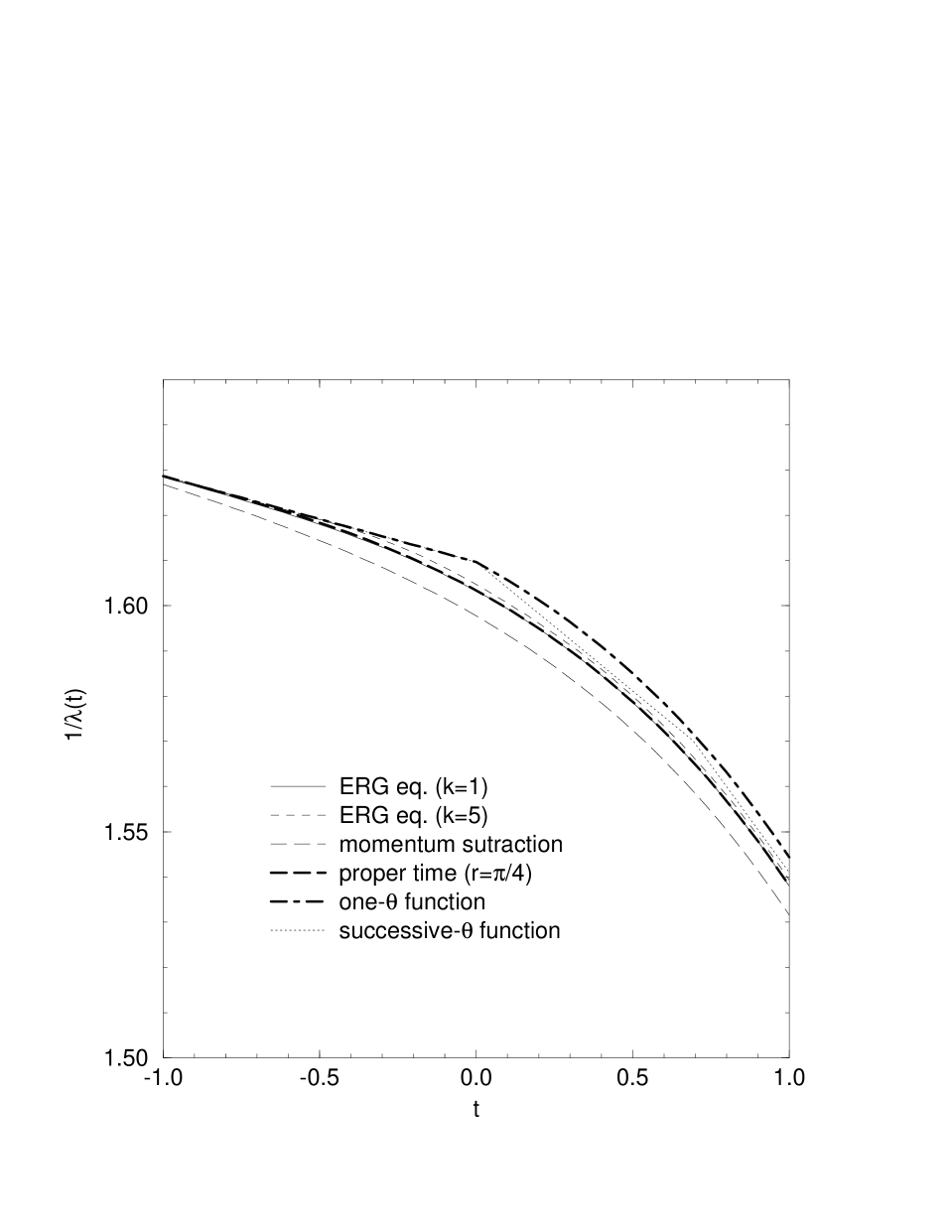
Figure 12: A magnified figure of fig. 11 near the threshold region.

So the maximal difference in this regime is $O(0.8)(\lambda/4\pi)$. Above $t=2$, which means above the $7$th Kaluza-Klein excitation, the maximal difference including the zero scheme is $O(0.08)(\lambda/4\pi)$.

4.2 Correction to gauge coupling unification

Now we would like to apply our result in the previous sections to the running of the gauge couplings. Here we will consider only the PT and one-$\theta$ function approximation schemes, because, as we have seen, the other schemes yield similar results. Suppose that the one-loop $\beta$-function of a gauge coupling $g_{\rm PT}$ has the form

$$16\pi^{2}\beta_{\rm PT}=g^{3}_{\rm PT}\left\{~{}b+\tilde{b}~{}\left[~{}\vartheta_{3}^{\delta}\left(\frac{ir}{\pi(R\Lambda)^{2}}\right)-1~{}\right]~{}\right\}$$ (84)

in the PT scheme with the normalization used in ref. [5] (i.e. $r=\pi(X_{\delta})^{-2/\delta}$ with $X_{\delta}=\pi^{\delta/2}/\Gamma(1+\delta/2)$), where the function $\vartheta_{3}(ir/\pi(R\Lambda)^{2})$ is given in eq. (73). The constant $b$ accounts for the massless modes and $\tilde{b}$ for the massive Kaluza-Klein modes. Since, as we can see in fig. 7, $\vartheta_{3}(ir/\pi(R\Lambda)^{2})$ for $\ln(R\Lambda)\mathrel{\mathchoice{\vbox{\offinterlineskip\halign{$\m@th\displaystyle\hfil#\hfil$\cr>\crcr\sim\crcr} }}{\vbox{\offinterlineskip\halign{$\m@th\textstyle\hfil#\hfil$\cr>\crcr\sim\crcr} }}{\vbox{\offinterlineskip\halign{$\m@th\scriptstyle\hfil#\hfil$\cr>\crcr\sim\crcr} }}{\vbox{\offinterlineskip\halign{$\m@th\scriptscriptstyle\hfil#\hfil$\cr>\crcr\sim\crcr} }}}T$ can be well approximated $(\pi/r)^{\delta/2}(R\Lambda)^{\delta}$, we replace the r.h.side of eq. (84) by

$$16\pi^{2}\beta_{\rm PT} \simeq g^{3}_{\rm PT}\left\{b-\tilde{b}+\tilde{b}\left[\vartheta_{3}^{\delta}\left(\frac{ir}{\pi(R\Lambda)^{2}}\right)\theta(T-\ln(R\Lambda))\right.\right.$$ (85)

$$\left.\left.+\left(\frac{\pi}{r}\right)^{\delta/2}(R\Lambda)^{\delta}\theta(\ln(R\Lambda)-T)\right]\right\}~{},$$

where $T$ is some value $\mathrel{\mathchoice{\vbox{\offinterlineskip\halign{$\m@th\displaystyle\hfil#\hfil$\cr>\crcr\sim\crcr} }}{\vbox{\offinterlineskip\halign{$\m@th\textstyle\hfil#\hfil$\cr>\crcr\sim\crcr} }}{\vbox{\offinterlineskip\halign{$\m@th\scriptstyle\hfil#\hfil$\cr>\crcr\sim\crcr} }}{\vbox{\offinterlineskip\halign{$\m@th\scriptscriptstyle\hfil#\hfil$\cr>\crcr\sim\crcr} }}}0$ in the asymptotic regime. This $\beta$-function yields the evolution of $g_{\rm PT}$

$$\frac{16\pi^{2}}{g_{\rm PT}^{2}(\Lambda)}-\frac{16\pi^{2}}{g_{\rm PT}^{2}(\Lambda_{0})}\simeq-b\ln\frac{\Lambda}{\Lambda_{0}}+\tilde{b}\ln(R\Lambda)-\tilde{b}\left\{\frac{(\pi/r)^{\delta/2}}{\delta}[(R\Lambda)^{\delta}-1]+\Delta_{\delta}\right\},$$ (86)

for $\Lambda>(1/R)e^{T}>1/R$, where

$$\Delta_{\delta}=T+\frac{(\pi/r)^{T\delta/2}}{\delta}(1-e^{\delta})+\int_{-T_{0}}^{T}dt\left[~{}\vartheta_{3}^{\delta}\left(\frac{ire^{-2t}}{\pi}\right)-1~{}\right]~{},$$ (87)

where we can replace $T_{0}$ by $-\infty$ as long as $T_{0}\ll 0$. Since $T$ is in the asymptotic regime, $\Delta_{\delta}$ does not depend on $T$. The $\Delta_{\delta}$ is the Kaluza-Klein threshold effect and we find for instance

$$\Delta_{\delta}(r=\pi(X_{\delta})^{-2/\delta}) \simeq \left\{\begin{array}[]{c}0.33\\ 0.55\end{array}\right.~{}~{}\mbox{for}~{}~{}\delta=\left\{\begin{array}[]{c}1\\ 2\end{array}\right.~{}.$$ (92)

It depends however on $r$, e.g.

$$\Delta_{1}(r=1) \simeq 0.22~{},~{}\Delta_{1}(r=2)\simeq 0.050~{},~{}\Delta_{1}(r=\pi)\simeq 0.023~{}.$$ (93)

$\Delta_{\delta}$ decreases for increasing $r$ and reaches at its minimum for $r=\pi$. So the $\pi$-scheme (defined by $r=\pi$) might be the most economic scheme, because one might neglect the threshold effect completely in this scheme. This can be seen by calculating the difference

$$\Delta_{\delta}(r)-\Delta_{\delta}(r^{\prime}) = \frac{1}{\delta}~{}[~{}(\frac{\pi}{r})^{\delta/2}-(\frac{\pi}{r^{\prime}})^{\delta/2}~{}]+\frac{1}{2}\ln\frac{r}{r^{\prime}}~{}.$$ (94)

Differentiating the r.h.side with respect to $r$, we find that $\Delta_{\delta}(r)$ becomes minimal at $r=\pi$. This dependence of $r$ is unphysical because we can absorb it into a redefinition of the coupling, or equivalently into a redefinition of $\Lambda$, as we will see.

It is now straightforward to apply the above formula to investigate the threshold effect to gauge coupling unification. To be definite, we consider the Kaluza-Klein model proposed in ref. [5], the MSSM with the Kaluza-Klein towers only in the gauge and Higgs supermultiplets. The gauge coupling $\beta$-functions are given by [5]

$$\left\{\begin{array}[]{l}b_{1}=33/5\\ b_{2}=1\\ b_{3}=-3\end{array}\right.~{}~{}\mbox{and}~{}~{}\left\{\begin{array}[]{l}\tilde{b}_{1}=3/5\\ \tilde{b}_{2}=-3\\ \tilde{b}_{3}=-6\end{array}\right.~{}.$$ (101)

As usual we use the $\alpha_{1}(M_{Z})~{}(=g_{1}^{2}(M_{Z})/4\pi)$ and $\alpha_{2}(M_{Z})$ as the input, and predict $\alpha_{3}(M_{Z})$ and $M_{\rm GUT}$. We find that threshold effect changes the unification scale as

$$\left(\frac{b_{1}-b_{2}}{\tilde{b}_{1}-\tilde{b}_{2}}-1\right)\ln\frac{M_{\rm GUT}^{(\theta)}}{M_{\rm GUT}^{({\rm PT})}}+\frac{(\pi/r)^{\delta}}{\delta}~{}R^{\delta}~{}\left[~{}(M_{\rm GUT}^{(\theta)})^{\delta}-(M_{\rm GUT}^{({\rm PT})})^{\delta}~{}\right]-\Delta_{\delta}=0~{},$$ (102)

where $M_{\rm GUT}^{(i)}$ is the unification scale in the $i$ scheme. Since $\Delta_{\delta}$ (which is given in eq. (87)) and the factor in front of $\ln$ in eq. (102) are positive, the unification scale in the PT scheme with $r=\pi/4$ is smaller than the one without the Kaluza-Klein threshold effect. For the model at hand the difference is only $\sim 1$ %.

The prediction of $\alpha_{3}(M_{Z})$ does not changes practically; there is a compensating mechanism. As we have observed, $M_{\rm GUT}^{(\theta)}$ is slightly larger that $M_{\rm GUT}^{({\rm PT})}$, which means that $\alpha_{3}(1/R)$ in the one-$\theta$ function approximation scheme with $M_{\rm GUT}^{(\theta)}$ is larger as compared with that of $M_{\rm GUT}^{({\rm PT})}$. Similarly, $\alpha_{3}(1/R)$ in the PT scheme with $M_{\rm GUT}^{({\rm PT})}$ is larger than the corresponding in the one-$\theta$ function approximation scheme with the same unification scale. These two effects are of the same magnitude. But it is clear that this compensating mechanism depends on the model. Since the threshold effect is

$$\delta\left(\frac{1}{\alpha}\right) \simeq ~{}\Delta_{\delta}~{}\frac{\tilde{b}}{4\pi}~{},$$ (103)

the effect could become in principle of the order of few percent in the PT scheme with $r=\pi/4$, i.e. comparable to the present experimental error [32].

The $r$-dependence in the prediction of $\alpha_{3}(M_{Z})$ should be absent. Let us see this explicitly at one-loop order. We start with the assumption that the unification condition

$$\frac{8\pi^{2}}{g_{{\rm GUT},r}^{2}(M_{\rm GUT}^{(r)})} = \frac{8\pi^{2}}{g_{r,i}^{2}(\Lambda_{0})}-b_{i}\ln\frac{M_{\rm GUT}^{(r)}}{\Lambda_{0}}+\tilde{b}_{i}\ln(RM_{\rm GUT}^{(r)})$$ (104)

$$-\tilde{b}_{i}\left\{\frac{(\pi/r)^{\delta/2}}{\delta}[(RM_{\rm GUT}^{(r)})^{\delta}-1]+\Delta_{\delta}(r)~{}\right\}~{}~{}\mbox{for all}~{}~{}i~{}$$

is satisfied in the $r$ scheme, where $\Lambda_{0}<1/R$ is the energy scale at which we match the unrenormalizable theory with a renormalizable effective theory , say in the $\overline{\mbox{MS}}$ scheme. We now would like to prove that the unification condition in the $r^{\prime}$ scheme as well is satisfied and that the $g_{3}^{2}(\Lambda_{0})$ prediction is $r$-independent. Comparing the asymptotic behavior of the couplings of two schemes, we first find that the unification scales are related by

$$M_{\rm GUT}^{(r^{\prime})} = M_{\rm GUT}^{(r)}(\frac{r^{\prime}}{r})^{1/2}~{}.$$ (105)

Then using the identity (94), we can rewrite the r.h.side of eq. (104) as

$$\frac{8\pi^{2}}{g_{r,i}^{2}(\Lambda_{0})}-\frac{1}{2}b_{i}\ln\frac{r}{r^{\prime}}-b_{i}\ln\frac{M_{\rm GUT}^{(r^{\prime})}}{\Lambda_{0}}+\tilde{b}_{i}\ln(RM_{\rm GUT}^{(r^{\prime})})$$

$$-\tilde{b}_{i}\left\{\frac{(\pi/r^{\prime})^{\delta/2}}{\delta}[(RM_{\rm GUT}^{(r^{\prime})})^{\delta}-1]+\Delta_{\delta}(r^{\prime})~{}\right\}+~{}~{}\mbox{for all}~{}~{}i~{},$$ (106)

where the sum of the first two terms is nothing but

$$\frac{8\pi^{2}}{g_{r^{\prime},i}^{2}(\Lambda_{0})} = \frac{8\pi^{2}}{g_{r,i}^{2}(\Lambda_{0})}-\frac{1}{2}b_{i}\ln\frac{r}{r^{\prime}}~{},$$ (107)

which can be obtained by computing the corresponding diagrams for $\Lambda_{0}<1/R$ in two different PT schemes. This shows the $r$-dependence in one-loop order. To match $g_{r,i}(\Lambda_{0})$ with $g_{\overline{\mbox{MS}}}(\Lambda_{0})$, we still have to clarify the relation between the $\overline{\mbox{MS}}$ scheme and the PT scheme in the MSSM. This is certainly outside of the scope of this paper, and we would like to leave it for future work .

4.3 Comparing with the string Kaluza-Klein threshold effect

String theories in general contain different kinds of towers of massive modes; the original massive string modes, the massive winding modes and the massive Kaluza-Klein modes. Their characteristic mass scale is, respectively, $O(1/\sqrt{\alpha^{\prime}})$, $O(1/R)$ and $(R/\sqrt{\alpha^{\prime}})O(1/\sqrt{\alpha^{\prime}})$, where $\alpha^{\prime}$ is the Regge slope. These massive states give rise to quantum contributions to the gauge couplings , and in the case of the hierarchal mass relation, that is, if $1/R\ll 1/\sqrt{\alpha^{\prime}}$, the Kaluza-Klein states are lighter than the others, so that one can expect that the Kaluza-Klein modes will give dominant contributions to the quantum effect [11, 12]. To be definite, in what follows we consider the weakly coupled heterotic string theory. The quantum corrections in this theory have been calculated [33, 34], and their form is given by

$$\frac{8\pi^{2}}{g_{s}^{2}} = \frac{8\pi^{2}}{g_{{\rm ST},i}^{2}}(M_{s})=\frac{8\pi^{2}}{g_{{\rm ST},i}^{2}}(Q)-b_{i}\ln\frac{M_{s}}{Q}-D_{i}~{},$$ (109)

where $D_{i}$ stands for the threshold effect of the massive states, and the string scale $M_{s}$ is related to $\alpha^{\prime}$ through [33]

$$M_{s} = \frac{\zeta}{\sqrt{\alpha^{\prime}}}~{},~{}\zeta=2\exp[(1-\gamma_{E})/2]3^{-3/4}(2\pi)^{-1/2}\simeq 0.432~{}.$$ (110)

We assume that the six dimensions are compactified on a six dimensional orbifold, so that the contribution to $D_{i}$ comes only from the massive supermultiplets forming a $N=2$ but not $N=4$ supermultiplet. In the hierarchal mass relation, $1/R\ll 1/\sqrt{\alpha^{\prime}}$, the contribution to $D_{i}$ for $Q\ll M_{s}$ is dominated by the Kaluza-Klein modes, and it can be written as [12]

$$D_{i}=\frac{1}{2}\tilde{b}_{i}\int_{-1/2}^{1/2}d\tau_{1}~{}\int_{\sqrt{1-\tau_{1}^{2}}}^{\infty}\frac{d\tau_{2}}{\tau_{2}}~{}\left\{~{}\sum_{m_{1},m_{2}\in{\bf Z}}\exp\left[~{}-\frac{\pi\tau_{2}\alpha^{\prime}}{R^{2}}(m_{1}^{2}+m_{2}^{2})~{}\right]-1\right\}~{},$$ (111)

where we have assumed that the radii associated with the two-dimensional torus embedded in the six-dimensional torus are both $R$, and $\tau=\tau_{1}+i\tau_{2}$ is the modulus of the word sheet torus corresponding to the one-loop word sheet topology. Making the change of the variable, $\tau_{2}\to t=\alpha^{\prime}\tau_{2}$, we obtain

$$D_{i} = \frac{1}{2}\tilde{b}_{i}\int_{-1/2}^{1/2}d\tau_{1}~{}\int_{\alpha^{\prime}\sqrt{1-\tau_{1}^{2}}}^{\infty}\frac{dt}{t}~{}\left\{~{}\sum_{m_{1},m_{2}\in{\bf Z}}\exp\left[~{}-\frac{\pi t}{R^{2}}(m_{1}^{2}+m_{2}^{2})~{}\right]-1\right\}$$ (112)

$$= \frac{1}{2}\tilde{b}_{i}\int_{-1/2}^{1/2}d\tau_{1}~{}\int_{\alpha^{\prime}\sqrt{1-\tau_{1}^{2}}}^{\infty}\frac{dt}{t}~{}\left\{\vartheta_{3}^{2}\left(\frac{it}{R^{2}}\right)-1\right\}~{}.$$

Then we interpret eq. (112) as a result of the “running” of $g_{{\rm ST},i}$ from $1/R$ to $M_{s}=\zeta/\sqrt{\alpha^{\prime}}$. The corresponding $\beta$-function may be obtained from

$$\beta_{{\rm ST},i} = \Lambda\frac{d}{d\Lambda}g_{{\rm ST},i}(M_{s}=\Lambda)$$ (113)

$$= \frac{g_{{\rm ST},i}^{3}}{16\pi^{2}}~{}\left\{b_{i}+\tilde{b}_{i}\int_{-1/2}^{1/2}d\tau_{1}~{}\left[~{}~{}\vartheta_{3}^{2}\left(\frac{i\sqrt{1-\tau_{1}^{2}}\zeta^{2}}{(\Lambda R)^{2}}\right)-1~{}\right]~{}\right\},$$

where $\zeta$ is given in eq. (110). Comparing this with eq. (84) we see that the $\tau_{1}$ integral averages the field theory results in different regularizations with a definite weight. Therefore, the string scheme corresponds to an average scheme, and by investigating the $\beta$-function in the asymptotic regime we can find the effective regularization scheme of, as we shall do below. We find that for $R\Lambda\gg 1$

$$\beta_{{\rm ST},i} \simeq g_{{\rm ST},i}^{3}\{b_{i}+\tilde{b}_{i}~{}G_{2}~{}(R\Lambda)^{2}~{}\},$$ (114)

where

$$~{}G_{\delta} = \frac{1}{\zeta^{\delta}}\int_{-1/2}^{1/2}d\tau_{1}~{}(1-\tau_{1}^{2})^{\delta/4}~{}=\frac{\pi}{3\zeta^{2}}\simeq 5.60~{}\mbox{for}~{}~{}\delta=2~{}.$$ (115)

According to the discussion in section 2 (see eq. (11)), the couplings in the PT scheme in the normalization of ref. [5] ($r=1$ for $\delta=2$) and in the string theory are related by

$$\frac{8\pi^{2}}{g_{{\rm PT},}^{2}} = \frac{8\pi^{2}}{g_{{\rm ST},}^{2}}-\frac{\pi}{2}(1-\frac{1}{3\zeta^{2}})(R\Lambda)^{2}~{}.$$ (116)

Equivalently, the scale parameters in the two schemes are related by $\Lambda_{\rm ST}=\sqrt{3}\zeta\Lambda_{\rm PT}$, implying that the unification scales in the two schemes are also related in the same way:

$$M_{s} = \sqrt{3}\zeta M_{\rm GUT}^{\rm(PT)}\simeq 0.748M_{\rm GUT}^{\rm(PT)}~{}.$$ (117)

As a next task we would like to compute the Kaluza-Klein threshold effect in the same way as in eq. (86). We find that

$$\frac{8\pi^{2}}{g_{\rm ST}^{2}(\Lambda)}-\frac{8\pi^{2}}{g_{\rm ST}^{2}(1/R)} \simeq -(b-\tilde{b})~{}\ln(R\Lambda)-\tilde{b}~{}\left\{~{}\frac{\pi}{6\zeta^{2}}~{}[~{}(R\Lambda)^{2}-1~{}]+\Delta_{\rm ST}~{}\right\}~{},$$ (118)

for $\Lambda>(1/R)e^{T}>1/R$, where (see also ref. [12])

$$\Delta_{\rm ST} = T+\frac{\pi}{6\zeta^{2}}(1-e^{2T})+\int_{-\infty}^{T}dt~{}\int_{-1/2}^{1/2}d\tau_{1}[~{}\vartheta_{3}^{2}(i\sqrt{1-\tau_{1}^{2}}\zeta^{2}e^{-2t})-1~{}]$$ (119)

$$\simeq 1.46~{}.$$

Since the string theory can be effectively regarded as the PT scheme with

$$r = 3\zeta^{2}~{},$$ (120)

as we can see from eq. (118), we would like to compare the threshold effect given in eq. (119) with that in this scheme. We find

$$\Delta_{\rm PT}(r=3\zeta^{2}) = T+\frac{\pi}{6\zeta^{2}}(1-e^{2T})\int_{-\infty}^{T}dt\left[~{}\vartheta_{3}^{2}\left(\frac{i3\zeta^{2}e^{-2t}}{\pi}\right)-1~{}\right]$$ (121)

$$\simeq 1.46~{}.$$

So we may conclude that the effective theory with $r=3\zeta^{2}$ can accurately describe the string theory for the case $M_{s}\gg 1/R$.

5 Summary and discussion

The higher dimensional theories, as a possible framework able in principle to unify all interactions, have a very long history starting from the work of Kaluza and Klein in the twenties and will certainly continue in the next century. In particular during the last thirty years there is a lot of theoretical interest in the various higher dimensional schemes, while recently we have witnessed an increasing interest due to the possibility that might be observable experimental consequences related to some large compactification radii. Apart from the well known field theory limit of string theories (see e.g. ref. [35]), there have been made many attempts to consider Yang Mills Theories in higher dimensions (see e.g. refs. [36]-[39] and references therein) with most well known those of the supergravity framework [39]. Maybe to the extend one is interested mainly in the low energy properties in four dimensions of a gauge theory defined in higher dimensions an elegant reduction scheme is the Coset Space one [37, 38].

Gauge theories in higher dimensions are (perturbatively) non-renormalizable by power counting. However to the extend that a higher dimensional theory is defined at weak coupling, it has been suggested in ref. [15] and in the present paper that the ERG provides us with a natural framework to study also the quantum behavior of the theory. The ERG approach based on the Wilson RG is indeed appropriate for dealing with higher dimensional gauge theories since its formulation is independent of dimensions and permits us to compute radiative corrections in a meaningful fashion.

As we have emphasized, the scale parameter introduced there (see eq. (18)) is the infrared cutoff parameter and indicates the energy scale at which the effective theory is defined. The RG equation (22) describes the flow of the effective theory as $\Lambda$ varies, and it reduces in the weak coupling limit in the derivative expansion approximation to the evolution equation of the coupling. We have also considered other schemes such as the momentum subtraction (MOM) scheme and the proper time (PT) regularization scheme. In the PT scheme the scale parameter $\Lambda$ is nothing but the ultraviolet cutoff parameter. Within this scheme it is indeed difficult to understand that the coupling “runs” with $\Lambda$. However, comparing all the schemes we have seen that the ultraviolet cutoff parameter introduced in the PT scheme and the subtraction scale introduced in the MOM scheme are just the scale parameter of the ERG, and moreover, that these regularization schemes give very similar results as far as the evolution of the coupling is concerned if one carefully eliminates the apparent regularization scheme dependence. We have arrived at the conclusion that the Kaluza-Klein threshold effect can be very small in certain regularization schemes; e.g., it is minimum for the $\pi$-scheme among the PT schemes. This feature of the Kaluza-Klein thresholds originates from the fact that, contrary to the renormalizable case, the lowest order $\beta$-function is regularization scheme dependent.

In a concrete application of our results we found that in fact the prediction of $\alpha_{3}(M_{Z})$ resulting from gauge coupling unification in the MSSM with the Kaluza-Klein tower only in the gauge and Higgs supermultiplets [5] does not change practically, in accord with the result of ref. [5]. We have also compared the Kaluza-Klein threshold effect in a string theory and its effective field theory, and we found that the string theory result averages those of the field theory in different regularizations, defining therefore an average regularization scheme of the effective theory. Surprisingly, the Kaluza-Klein threshold effect calculated in the effective theory with the average regularization can very well approximate the corresponding string theory result.

Acknowledgments
Two of the authors (J.K and G.Z.) thank Alex Pomarol for discussions and the organigers of the Summer Institute ’99 at Yamanashi, which gave the opportunity for extended discussions on the present work.

References

- [1]
- [2] I. Antoniadis, Phys. Lett. B246 (1990) 377; I. Antoniadis, C. Muñoz and M. Quirós, Nucl. Phys. B397 (1983) 515; I. Antoniadis and K. Benakli, Phys. Lett. B326 (1994) 69; I. Antoniadis, K. Benakli and M. Quirós, Phys. Lett. B331 (1994) 313.
- [3] I. Antoniadis and M. Quiros, Phys. Lett. B392 (1997) 61; I. Antoniadis, N. Arkani-Hamed, S. Dimopoulos and G. Dvali, Phys. Lett. B429 (1998) 263.
- [4] I. Antoniadis, N. Arkani-Hamed, S. Dimopoulos and G. Dvali, Phys. Lett. B436 (1998) 257.
- [5] K. Dienes, E. Dudas and T. Gherghetta, Phys. Lett. B436 (1998) 311; Nucl. Phys. B537 (1999) 47.
- [6] E. A. Mirabelli et. al., Phys. Rev. Lett. 82 (1999) 2236; G. F. Giudice et. al., Nucl. Phys. B544 (1999) 3; G. Shiu et. al., Phys. Lett. B458 (1999) 274; K. Cheung, hep-ph/9904266; P. Mathews et. al., Phys. Lett. B455 (1999) 115; hep-ph/9904232; G. Dvali, A. Yu. Smirnov, hep-ph/9904211; A. Ioannisian, A. Pilaftsis, hep-ph/9907522; Z. K. Silagadge, hep-ph/9907328.
- [7] G. Shiu and S.-H. H. Tye, Phys. Rev. D58 (1998) 106007; Z. Kakushadze and S.-H. H. Tye, Nucl. Phys. B548 (1999) 180.
- [8] C. Bachas, JHEP 9811 (1998) 023; Z. Kakushadze, Nucl. Phys.B548 (1999) 205; A. Domini, S. Rigolin, Nucl. Phys. B550 (1999) 59.
- [9] I. Antoniadis, C. Bachas and E. Dudas, hep-ph/9906039.
- [10] T.R. Taylor and G. Veneziano, Phys. Lett. B212 (1988) 147.
- [11] Z. Kakushadze and T. R. Taylor, hep-ph/9905137.
- [12] D. Ghilencea and G. G. Ross, hep-ph/9908369.
- [13] D. Ghilencea and G. G. Ross, Phys. Lett. B442 (1998) 165.
- [14] A. Pomarol and M. Quiros, Phys. Lett. B438 (1998) 255; A. Delgado, A. Pomarol and M. Quiros, hep-ph/9812489; I. Antoniadis et. al., Nucl. Phys. B544 (1999) 503.
- [15] T. Kobayashi, J. Kubo, M. Mondragon and G. Zoupanos, Nucl. Phys. B550 (1999) 99.
- [16] T. E. Clark and S. T. Love, Phys. Rev. D60 (1999) 025005.
- [17] A. Perez-Lorenzana and R. N. Mohapatra, hep-ph/9904504; H-C. Cheng et. al., hep-ph/9906327; Y. Kawamura, hep-ph/9902423; K. Huitu and T. Kobayashi, hep-ph/9906431; H. Hatanaka, Prog. Theo. Phys. 102 (1999) 407; M. Sakamoto et. al., Phys. Lett. B458 (1999) 231; S. A. Abel and S. F. King, Phys. Rev. D59 (1999) 095010.
- [18] K. G. Wilson and J. Kogut, Phys. Rep. 12C (1974) 75; K. G. Wilson, Rev. Mod. Phys. 47 (1975) 773.
- [19] F. J. Wegner and A. Houghton, Phys. Rev. A8 (1973) 401.
- [20] J. Polchinski, Nucl. Phys. B231 (1984) 269.
- [21] C. Wetterich, Phys. Lett.B301 (1993) 90; M. Bonini, M. D’Attanasio and G. Marchesini, Nucl. Phys. B409 (1993) 441.
- [22] D. O’ Connor and C. R. Stephens, Phys. Rev. Lett. 72 (1994) 506; Int. J. Mod. Phys. A9 (1994) 2805.
- [23] J. F. Nicol, T. S. Chang and H. E. Stanley, Phys. Rev. Lett. 33 (1974) 540.
- [24] N. Tetradis and C. Wetterich, Nucl. Phys. B422 (1994) 541; B398 (1993) 659; J. Berges et. al., Phys. Lett. B393 (1997) 387; Phys. Rev. Lett. 77 (1996) 873;
- [25] T. R. Morris, Phys. Lett. 329 (1994) 241; Nucl. Phys. B409 (1997) 363; T. R. Morris and M. D. Turner, Nucl. Phys. B509 (1998) 637;
- [26] K.-I. Aoki et. al., Prog. Theor. Phys. 95 (1996) 409; Prog. Theor. Phys. 99 (1998) 451;
- [27] T. R. Morris, Int. J. Mod. Phys. A9 (1994) 2411; K.-I. Aoki et. al., Scheme Dependence of the Wilsonian Effective Action and Sharp Cutoff Limit of the Flow Equation, in preparation.
- [28] N. Tetradis and C. Wetterich, Nucl. Phys. B398 (1993) 659; S-B. Liao, J. Polonyi and D. Xu, Phys. Rev. D51 (1995) 748.
- [29] Y. Yamada, Phys. Rev. D50 (1994) 3537; J. Hisano and M. Shifman, Phys. Rev. D56 (1997) 5475; I. Jack and D. R. T. Jones, Phys. Lett. B415 (1997) 383; I. Jack et. al., Phys. Lett. B426 (1998) 73; L. V. Andeev et. al., Nucl. Phys. B510 (1998) 289; D. I. Kazakov, Phys. Lett. B421 (1998) 211; T. Kobayashi et. al., Phys. Lett. B427 (1998) 291; I. Jack et. al., Phys. Lett. B432 (1998); N. Arkani-Hamed et. al., Phys. Rev. D58 (1998) 115005; A. Karch et. al., Phys. Lett. B441 (1998) 235; M. A. Luty and R. Rattazzi, hep-th/9908085.
- [30] P. M. Stevenson, Phys. Lett. B100 (1981) 61; Phys. Rev. D23 (1981) 2916.
- [31] D. A. Ross, Nucl. Phys. B140 (1978) 1; J. Ellis et. al., Nucl. Phys. 176 (1980) 61; J. Kubo and S. Sakakibara, Phys. Lett. B103 (1981) 39.
- [32] C. Caso et. al., The Review of Particle Physics, The European Physical Journal C3 (1998) 1.
- [33] V. Kaplunovsky, Nucl. Phys. B307 (1988) 145; Erratum: Nucl. Phys. B382 (1992) 436;
- [34] K. Choi, Phys. Rev. D37 (1988) 1564; L. Dixon, V. Kaplunovsky and J. Louis, Nucl. Phys. B355 (1991) 649; V. Kaplunovsky and J. Louis, Nucl. Phys. B444 (1995) 191; I. Antoniadis, K. Narrain and T. Taylor, Phys. Lett. B267 (1991) 37; I. Antoniadis, E. Gava and K. Narrain, Nucl. Phys. B383 (1992) 93; E. Kiritisis and C. Kounnas, Nucl. Phys. B442 (1995) 472; S. Ferrara, C. Kounnas, D. Lüst and F. Zwirner, Nucl. Phys. B365 (1991) 431; P. Mayr and S. Stieberger, Nucl. Phys. B407 (1993) 725; D. Bailin, A. Love, W. A. Sabra and S. Thomas, Mod. Phys. Lett. A9 (1994) 67; Mod. Phys. Lett. A10 (1995) 337; P. Mayr, H. P. Nilles and S. Stieberger, Phys. Lett. B317 (1993) 53; P. Mayr and S. Stieberger, Phys. Lett. B355 (1995) 107; G. L. Cardoso, D. Lüst and T. Mohaupt, Nucl. Phys. B450 (1995) 115.
- [35] M. B. Green, J. H. Schwarz and E. Witten, Superstring Theory, Vols. I, II (Cambridge Univ. Press, Cambridge, 1987); D. Lüst and S. Theisen, Lectures on String Theory, Lecture Notes in Physics, Vol.346 (Springer, Heidelberg, 1989).
- [36] R. Coquereaux and A. Jadczyk, Riemannian Geometry, Fiber Bundles, Kaluza- Klein Theories ans All That…, (World Scientific, Singapore, 1998).
- [37] Y. A. Kubyshin, J. M. Mourao, G. Rudolph and I. P. Volobujev, Dimensional Reduction of Gauge Theories, Spontaneous Compactification and Model Building, Lecture Notes in Physics, Vol. 349 (Springer, Heidelberg, 1989); D. Kapetanakis and G. Zoupanos, Phys. Rept. 219 (1992) 1.
- [38] P. Forgacs and N. S. Manton, Commun. Math. Phys. 72 (1980) 15; N. S. Manton, Nucl. Phys. B193 (1981) 502; G. Chapline and R. Slansky, Nucl. Phys. B209 (1982) 461; S. Randjbar-Daemi, A. Salam and J. Strathdee, Phys. Lett. B132 (1982) 56; C. Wetterich, Nucl.Phys. B222 (1983) 20; K. Pilch and A. N. Schellekens, Nucl. Phys. B256 (1985) 109; P. Forgacs, Z. Horvath and L. Palla, Z.Phys. C30 (1986) 261; K. Farakos et. al. Phys. Lett. B191 (1987) 128; G. Zoupanos, Phys.Lett. B201 (1988) 301; D. Kapetanakis and G. Zoupanos Phys. Lett. B 232 (1989) 104; Phys. Lett. B249 (1990) 66; Phys. Lett. B249 (1990) 73; Z. Phys. C56 (1992) 91.
- [39] M. J. Duff, B. Nillson and C. Pope, Phys. Rept. 130 (1986) 1.