Analysis of a three flavor neutrino oscillation fit to recent Super-Kamiokande data

Abstract

We have analyzed the most recent available Super-Kamiokande data in a three flavor neutrino oscillation model. We have here neglected possible matter effects and performed a fit to atmospheric and solar Super-Kamiokande data. We have investigated a large parameter range, where the mixing angles were restricted to $0\leq\theta_{i}\leq\pi/2$, $i=1,2,3$, and the mass squared differences were taken to be in the intervals $10^{-11}\;{\rm eV}^{2}\leq\Delta m^{2}\leq 10^{-2}\;{\rm eV}^{2}$ and $10^{-4}\;{\rm eV}^{2}\leq\Delta M^{2}\leq 10\;{\rm eV}^{2}$. This yielded a best solution characterized by the parameter values $\theta_{1}\simeq 45^{\circ}$, $\theta_{2}\simeq 10^{\circ}$, $\theta_{3}\simeq 45^{\circ}$, $\Delta m^{2}\simeq 4.4\times 10^{-10}\;{\rm eV}^{2}$, and $\Delta M^{2}\simeq 1.01\times 10^{-3}\;{\rm eV}^{2}$, which shows that the analyzed experimental data speak in favor of a bimaximal mixing scenario with one of the mass squared differences in the “just-so” domain and the other one in the range capable of providing a solution to the atmospheric neutrino problem.

I Introduction

Most of the analyses concerning neutrino oscillations have so far been done within the framework of the theory of two flavor neutrino oscillation. In these scenarios, the observed deficit of solar electron neutrinos is usually explained by means of $\nu_{e}\leftrightarrow\nu_{\mu}$ oscillations, whereas the lack of atmospheric muon neutrinos is interpreted as a consequence of $\nu_{\mu}\leftrightarrow\nu_{\tau}$ oscillations. The main advantage of the two flavor oscillation scenario is that the oscillation probability depends on only two parameters, the mass squared difference $\Delta m^{2}$ and the mixing angle $\theta$.

Recently, it was pointed out by several authors, that in some cases the interpretation of the experimental data in terms of two flavor oscillations might yield misleading and sometimes even wrong results (see e.g. Ref.[1]) and that a three flavor oscillation description is to be favored. Unfortunately, the oscillation probabilities depend in this case on five parameters, two mass squared differences and three mixing angles, which makes it quite hard to deal with the dependence of the probability functions on these parameters.

The most popular three flavor neutrino oscillation scenario is the so called bimaximal mixing scenario [2], where two of the mixing angles are maximal, i.e., they have values of about $45^{\circ}$, whereas the remaining one is restricted by the CHOOZ experiment to be rather small at least for certain parameter ranges [3]. The three flavor oscillation scenario can then be shown to decouple into two distinct scenarios involving two flavors, in which case it is of course much easier to perform a fit to the experimental data. Many authors [4] use the CHOOZ result to simplify the oscillation probability formulas for three flavors and then perform a fit of the two decoupled two flavor neutrino oscillation scenarios to the experimental data.

In this paper, we will present a numerical fit within a three flavor neutrino mixing scenario to the zenith angle distribution of 850 day atmospheric neutrino Super-Kamiokande data and 708 day solar neutrino Super-Kamiokande data. However, we will not make any assumptions about the parameters on which the oscillation probability formulas depend, i.e., we fit the scenario in the most general case and for a large parameter range to the experimental data.

The paper is organized as follows. In Sec. II, we summarize the basic features of three flavor neutrino oscillation theory. In Sec. III, we present the choice of experimental data and in Sec. IV, we discuss the minimization procedure. In Sec. V, we give the obtained solutions of the minimization problem, which are interpreted in Sec. VI. The fits corresponding to the solutions are discussed and compared in Sec. VII and then these solutions are tested for stability in Sec. VIII. Finally, Sec. IX contains a summary and our conclusions.

II Theory of Three Flavor Neutrino Oscillations

In three flavor neutrino oscillation theory one assumes the neutrino states with definite flavor $|\nu_{\alpha}\rangle$, $\alpha=e,\mu,\tau$, to be linear superpositions of states with definite mass $|\nu_{i}\rangle$, $i=1,2,3$,

$$|\nu_{\alpha}\rangle=\sum_{i=1}^{3}U_{\alpha i}^{*}|\nu_{i}\rangle,\quad\alpha=e,\mu,\tau.$$ (1)

The unitary mixing matrix $U$ is called Cabibbo–Kobayashi–Maskawa (CKM) matrix and can generally be parameterized by three mixing angles $\theta_{i}$, where $i=1,2,3$, and three CP-violating phases. One of the latter were recently claimed to be observable by next generation neutrino detectors [5] and could lead to physically very interesting consequences. The other two can be shown to cause no physical effects. However, for this analysis these phases are too small to be important and we will neglect them in what follows. This implies $U_{\alpha i}=U_{\alpha i}^{*}$ and therefore we can write the CKM matrix in its (real) standard parameterization [6] as

$$U=\left(\begin{matrix}c_{2}c_{3}&s_{3}c_{2}&s_{2}\\ -s_{3}c_{1}-s_{1}s_{2}c_{3}&c_{1}c_{3}-s_{1}s_{2}s_{3}&s_{1}c_{2}\\ s_{1}s_{3}-s_{2}c_{1}c_{3}&-s_{1}c_{3}-s_{2}s_{3}c_{1}&c_{1}c_{2}\end{matrix}\right),$$ (2)

where $s_{i}\equiv\sin\theta_{i}$ and $c_{i}\equiv\cos\theta_{i}$. The probability for detection of a neutrino of flavor $\beta$ in a beam of neutrinos consisting exclusively of flavor $\alpha$ at the source of the beam is for three flavors given by

$$P_{\alpha\beta}=\delta_{\alpha\beta}-4\mathop{\sum_{i=1}^{3}\sum_{j=1}^{3}}_{i<j}U_{\alpha i}U_{\beta i}U_{\alpha j}U_{\beta j}\sin^{2}\left(\frac{\Delta m^{2}_{ij}L}{4E}\right),\quad\alpha,\beta=e,\mu,\tau,$$ (3)

where $\delta_{\alpha\beta}$ is Kronecker’s delta, $L$ is the distance from the source to the detector, $E$ is the neutrino energy, and $\Delta m^{2}_{ij}$ is the difference between the squares of the masses corresponding to the mass eigenstates $|\nu_{i}\rangle$ and $|\nu_{j}\rangle$. Since

$$\Delta m^{2}_{21}+\Delta m^{2}_{32}+\Delta m^{2}_{13}=0$$ (4)

the mass squared differences are not linearly independent, and it is convenient to choose

$$\Delta m^{2} \equiv \Delta m^{2}_{21},$$ (5)

$$\Delta M^{2} \equiv \Delta m^{2}_{32},$$ (6)

from which follows that

$$\Delta m^{2}_{31}=-\Delta m^{2}_{13}=\Delta m^{2}+\Delta M^{2}.$$ (7)

So far we have considered the neutrino states to be plane waves, i.e., to have a definite momentum. Since the neutrino state is neither produced nor detected with a definite momentum or propagation length, one has to average over $L/E$ as well as other uncertainties in production and detection. We will here follow closely Ref. [1] and assume that these uncertainties to be described by a Gaussian average

$$\langle P_{\alpha\beta}\rangle=\int_{-\infty}^{\infty}P_{\alpha\beta}(x)f(x)dx,$$ (8)

where

$$f(x)=\frac{1}{\gamma\sqrt{2\pi}}\exp\left\{-\frac{(x-l)^{2}}{2\gamma^{2}}\right\}$$ (9)

and $x\equiv L/E$. Inserting formula (3) for $P_{\alpha\beta}$ yields

$$\langle P_{\alpha\beta}\rangle=\delta_{\alpha\beta}-2\mathop{\sum_{i=1}^{3}\sum_{j=1}^{3}}_{i<j}U_{\alpha i}U_{\beta i}U_{\alpha j}U_{\beta j}\left[1-\cos(2l\Delta m^{2}_{ij})\exp\{-2\gamma^{2}(\Delta m^{2}_{ij})^{2}\}\right],$$ (10)

where $l$ is given by

$$l\simeq 1.27\left\langle\frac{L}{E}\right\rangle\simeq 1.27\frac{\langle L\rangle}{\langle E\rangle}$$ (11)

and therefore related to the sensitivity of the experiment. $\langle L\rangle$ should here be inserted in meters, whereas $\langle E\rangle$ should be inserted in MeV. The parameter $\gamma$ is the so called damping factor and in accordance with Ref. [1] we will choose

$$\gamma=\frac{L}{E}\left(\frac{\Delta L}{L}+\frac{\Delta E}{E}\right),$$ (12)

where $\Delta E$ and $\Delta L$ are the uncertainties in neutrino energy and propagation length, respectively.

For large values of $\gamma$

$$\exp\{-2\gamma^{2}(\Delta m^{2}_{ij})^{2}\}\rightarrow 0$$

and the oscillation term vanishes. The transition probability then becomes a constant dependent on the values of the mixing angles; the oscillation is said to become “washed out”. To proceed, one now has to determine the values of the parameters $L,E,\Delta L,$ and $\Delta E$ for the experiments under consideration.

III Choice of Experimental Data

We are going to consider three types of Super-Kamiokande data, multi-GeV $e$-like atmospheric neutrino data, multi-GeV $\mu$-like atmospheric neutrino data, and solar neutrino data.

A Solar neutrino data

The probabilities were taken from Ref. [7] for 14 data points in an energy range from 6 MeV to 12 MeV. The probability is almost constant for all 14 data points. The path length for solar neutrinos is given by the distance from the Sun to Earth ($L\simeq 1.44\times 10^{11}$ m) and the uncertainty of the path length is here assumed to be negligible compared to $L$, i.e.,

$$\frac{\Delta L}{L}\simeq 0.$$ (13)

The damping factor then becomes

$$\gamma\simeq\frac{L}{E}\frac{\Delta E}{E},$$ (14)

where $\Delta E=0.5\;{\rm MeV}$ is the energy resolution of the experiment.

B Atmospheric neutrino data

The atmospheric neutrino data are divided into atmospheric multi-GeV $e$-like events and atmospheric multi-GeV $\mu$-like events. In both cases, the flux measurements are performed for five bins, i.e., for five different values

$$\cos\theta=-0.8,-0.4,0,0.4,0.8$$

of the zenith angle $\theta$, which is defined as the angle between the direction of the measurement and the axis through experiment and the middle of the Earth. Therefore, $\cos\theta=-1$ corresponds to straight upward going neutrinos, whereas for $\cos\theta=1$ the neutrinos are produced in the atmosphere right above the detector.

The experimental data used are 850 day Super-Kamiokande data and Monte Carlo no-oscillation predictions for 40 years generated lifetime for the five bins. The corresponding errors were taken from Ref. [8].

The results of the Super-Kamiokande experiment are usually presented by means of the “ratio of the ratios”

$${\cal R}=\frac{\Phi_{\mu}}{\Phi_{e}}(data)/\frac{\Phi_{\mu}}{\Phi_{e}}(MC),$$ (15)

where $\Phi_{\alpha}$ is the flux of neutrino flavor $\alpha$.

In Summer 1998, the Super-Kamiokande Collaboration published experimental values for this “ratio of the ratios” of ${\cal R}=0.63\pm 0.03(stat)\pm 0.05(sys)$ for sub-GeV events and ${\cal R}=0.65\pm 0.03(stat)\pm 0.08(sys)$ for multi-GeV events [9], which was the first direct observation of neutrino oscillations.

However, to be able to fit both, $e$-like and $\mu$-like data to the measurements, we will use here the directly measured disappearance rates

$$R_{e}=\frac{\Phi_{e}(data)}{\Phi_{e}(MC)}$$ (16)

for $e$-like events and

$$R_{\mu}=\frac{\Phi_{\mu}(data)}{\Phi_{\mu}(MC)}$$ (17)

for $\mu$-like events. The main disadvantage of this is the uncertainty in the expected neutrino flux, which was claimed to be up to 20$\%$ [10], due to the unknown flux of cosmic particles hitting the atmosphere. To handle this one can introduce an overall flux uncertainty factor $\eta$ with values between 0.8 and 1.2. The actual neutrino flux for the neutrino flavor $\alpha$ is then given by $\tilde{\Phi}_{\alpha}=\eta\Phi_{\alpha}$. Thus, in absence of neutrino oscillations, the ratio between the theoretical and the measured fluxes would just be $R_{\alpha}=\eta$, whereas otherwise one obtains

$$R_{\alpha}=\frac{\tilde{\Phi}_{e}P_{e\alpha}+\tilde{\Phi}_{\mu}P_{\mu\alpha}+\tilde{\Phi}_{\tau}P_{\tau\alpha}}{\Phi_{\alpha}},\quad\alpha=e,\mu,\tau,$$ (18)

where $P_{\alpha\beta}$ is the transition probability from $\alpha$ to $\beta$, see Sec. II. In what follows, we are going to neglect the $\tau$ contribution due to too small production cross sections. The uncertainty in the flux of cosmic rays is then an overall factor common to the ratios $R_{\alpha}$, where $\alpha=e,\mu$, of the both remaining neutrino flavors. Denoting $R\equiv\Phi_{\mu}/\Phi_{e}$, one obtains

$$R_{e}=\eta(P_{ee}+RP_{\mu\mu})$$ (19)

for the electron neutrino ratio and

$$R_{\mu}=\eta\left(P_{ee}+\frac{1}{R}P_{\mu\mu}\right)$$ (20)

for the muon neutrino ratio. The value of $R$ is theoretically well determined to be about $R\simeq 3$ at $E\simeq 10$ GeV [11].

The energy of the measured multi-GeV neutrinos is assumed to be $E=10$ GeV with negligible uncertainty compared to $E$ and we set $\Delta E/E\simeq 0$. The path length for a neutrino that was detected in a bin corresponding to the zenith angle $\theta$ is given by

$$L(\theta)=\sqrt{r^{2}\cos^{2}\theta+2rd+d^{2}}-r\cos\theta,$$ (21)

as is easily obtained from geometrical considerations. Here $r$ is the radius of the Earth and $d$ is the typical altitude of the neutrino production point in the atmosphere, which we assumed to be $d=10$ km. The uncertainty in path length is mainly determined by $\Delta\cos\theta=0.2$ and therefore

$$\Delta L=\left|\frac{\partial L(\theta)}{\partial\cos\theta}\right|\Delta\cos\theta=\frac{rL}{L+r\cos\theta}\;\Delta\cos\theta$$ (22)

The damping factor $\gamma$ is thus a function of $\theta$

$$\gamma\simeq\frac{\Delta L}{E}.$$ (23)

IV The Minimization Procedure

According to the last section, we have 24 data points, which we can use for the fit to the parameters of the theory: the five bins for $e$-like events, the five bins for $\mu$-like events, and the 14 data points for the solar neutrinos.

The function used to obtain the parameters is given by

$$\chi(\theta_{1},\theta_{2},\theta_{3},\Delta m^{2},\Delta M^{2}) = \frac{1}{{\rm w}_{tot}}\bigg{\{}\sum_{i=1}^{5}{\rm w}_{e,i}\frac{1}{R^{2}_{e,i}(exp)}\left[R_{e,i}-R_{e,i}(exp)\right]^{2}+\sum_{i=1}^{5}{\rm w}_{\mu,i}\frac{1}{R^{2}_{\mu,i}(exp)}\left[R_{\mu,i}-R_{\mu,i}(exp)\right]^{2}$$ (24)

$$+ \sum_{i=1}^{14}{\rm w}_{sun,i}\frac{1}{P^{2}_{sun,i}(exp)}\left[P_{sun,i}-P_{sun,i}(exp)\right]^{2}\bigg{\}},$$ (25)

where the first two sums run over the five bins and the third one over the 14 data points for the solar neutrinos. The weights have been taken as

$${\rm w}_{e,i} = R_{e,i}(exp)/\Delta R_{e,i}(exp),$$ (26)

$${\rm w}_{\mu,i} = R_{\mu,i}(exp)/\Delta R_{\mu,i}(exp),$$ (27)

$${\rm w}_{sun,i} = P_{sun,i}(exp)/\Delta P_{sun,i}(exp),$$ (28)

$${\rm w}_{tot} = \sum_{i=1}^{5}{\rm w}_{e,i}+\sum_{i=1}^{5}{\rm w}_{\mu,i}+\sum_{i=1}^{14}{\rm w}_{sun,i}.$$ (29)

The mixing angles were constrained to the interval $[0,\pi/2]$, whereas for the mass squared differences we assumed one of them to be in the range $10^{-11}\;{\rm eV}^{2}\leq\Delta m^{2}\leq 10^{-2}\;{\rm eV}^{2}$ and the other one in $10^{-4}\;{\rm eV}^{2}\leq\Delta M\leq 10\;{\rm eV}^{2}$. Since these large parameter ranges yield no numerically stable solution, we minimized function (25) for 45 parameter ranges corresponding to all combinations of values for the mass squared differences between

$$10^{-11}\;{\rm eV}^{2} \leq \Delta m^{2}\leq 10^{-10}\;{\rm eV}^{2},$$ (30)

$$10^{-10}\;{\rm eV}^{2} \leq \Delta m^{2}\leq 10^{-9}\;{\rm eV}^{2},$$ (31)

$$\vdots \hskip 28.45274pt\vdots$$ (32)

$$10^{-3}\;{\rm eV}^{2} \leq \Delta m^{2}\leq 10^{-2}\;{\rm eV}^{2}$$ (33)

for the small mass squared difference and

$$10^{-4}\;{\rm eV}^{2} \leq \Delta M^{2}\leq 10^{-3}\;{\rm eV}^{2},$$ (34)

$$10^{-3}\;{\rm eV}^{2} \leq \Delta M^{2}\leq 10^{-2}\;{\rm eV}^{2},$$ (35)

$$\vdots \hskip 28.45274pt\vdots$$ (36)

$$1\;{\rm eV}^{2} \leq \Delta M^{2}\leq 10\;{\rm eV}^{2}$$ (37)

for the larger one.

Following Ref. [1], we chose the following strategy to deal with the flux uncertainty factor $\eta$: During the search for minima of function (25), we set it equal to unity, i.e., we neglected the flux uncertainty. The solutions obtained in this way were then tested for their stability with respect to variations of $\eta$, see Sec. VIII.

To minimize the function $\chi$ in Eq. (25) we generated $N=10^{6}$ random values for each of the five parameters in the corresponding range such that we obtained $N$ values of the minimization function. After that we picked the parameter set that yielded the smallest value for the function and repeated this procedure $n=20$ times. Each of the obtained $n$ parameter sets then served as starting values for a deterministic minimization procedure, using a sequential quadratic programming method such that one obtains again $n$ parameter sets as an end result.

V Solutions of the Minimization Problem

The solutions to the minimization problem can best be obtained by considering tables like Table I, where the best point values for the two mass squared differences for each of the investigated mass regions are shown. One can see, that for most of the mass regions at least one of the two mass squared differences was obtained on one of the region boundaries. In this case, we assumed that the value of the corresponding mass squared difference converges towards a better minimum in one of the neighbor regions. Thus, a given parameter region was only considered to contain a solution to the minimization problem, if both values of the mass squared differences were obtained within the boundaries of the region. Note, that the values obtained for $\Delta M^{2}$ are almost randomly distributed in the last column of Table I, i.e., in the range $1\;{\rm eV}^{2}\leq\Delta M^{2}\leq 10\;{\rm eV}^{2}$. This is due to a too large value of the damping factor $\gamma$ in Eq. (10) such that the minimization function becomes independent of this parameter. Only $\Delta m^{2}$ and the mixing angles are in this case fitted to the experimental data.

To keep overview over the various considered parameter regions one can consider Table II. Here a region, where a value for $\Delta M^{2}$ was obtained within the boundaries, is marked with an “$M$”, whereas a region with a corresponding value for $\Delta m^{2}$ is marked with an “$m$”. One obtains in this way eight regions, marked “$M\;m$” in Table II, where the mass squared differences are within the region boundaries. Seven of these regions are contained in the first two rows of Table II, whereas the eighth one was obtained within the range $10^{-4}\;{\rm eV}^{2}\leq\Delta m^{2}\leq 10^{-3}\;{\rm eV}^{2}$, $1\;{\rm eV}^{2}\leq\Delta M^{2}\leq 10\;{\rm eV}^{2}$. The parameter values obtained from the minimization procedure with the mass squared differences constrained to these regions correspond to the possible solutions of the minimization problem. One notices that the regions marked with “$M\;m$” split Table II in three distinct areas, corresponding to three types of solutions, as we will see.

The first of these interesting areas is the one containing the parameter regions in the upper left corner of Table II, i.e., the nine regions in the range $\;10^{-11}\;{\rm eV}^{2}\leq\Delta m^{2}\leq 10^{-8}\;{\rm eV}^{2}$, $10^{-4}\;{\rm eV}^{2}\leq\Delta M^{2}\leq 10^{-1}\;{\rm eV}^{2}$. In this range, there are all together five possible solutions, i.e., mass regions, where the mass squared differences were obtained within the region boundaries. To pick the best of the possible solutions for this type, consider Table III, where the best point values for the minimization function (25) are shown. The smallest value of the minimization function was obtained in the region corresponding to $10^{-10}\;{\rm eV}^{2}\leq\Delta m^{2}\leq 10^{-9}\;{\rm eV}^{2}$, $10^{-3}\;{\rm eV}^{2}\leq\Delta M^{2}\leq 10^{-2}\;{\rm eV}^{2}$. In all surrounding regions, we obtained values for the minimization function, which are larger, such that there seems indeed to be a minimum in the region specified above. Thus, the corresponding parameter set is a solution of the minimization problem, and we will denote it by Solution 1 in what follows. Considering the rest of Table III, one can see that this solution corresponds to the smallest value of the minimization function in the whole investigated parameter range, which means that it provides the best fit to the experimental data, as will be seen in Sec. VII. Note that the value of the minimization function in the parameter range containing Solution 1 is very close to the one obtained in the region $10^{-10}\;{\rm eV}^{2}\leq\Delta m^{2}\leq 10^{-9}\;{\rm eV}^{2},\;10^{-4}\;{\rm eV}^{2}\leq\Delta M^{2}\leq 10^{-3}\;{\rm eV}^{2}$. Furthermore, the values for the mass squared differences obtained within these two regions are rather close to each other, and one can not really distinguish, if these two possible solutions correspond to the same minimum or to two distinct minima very close to each other.

The second interesting area of Table II contains six parameter regions in the range $10^{-5}\;{\rm eV}^{2}\leq\Delta m^{2}\leq 10^{-3}\;{\rm eV}^{2}$, $10^{-1}\;{\rm eV}^{2}\leq\Delta M^{2}\leq 10\;{\rm eV}^{2}$. Here a second type of solution is obtained in the region $10^{-4}\;{\rm eV}^{2}\leq\Delta m^{2}\leq 10^{-3}\;{\rm eV}^{2}$, $1\;{\rm eV}^{2}\leq\Delta M^{2}\leq 10\;{\rm eV}^{2}$, i.e., in the last column, eighth row of Table II. We will denote this solution by Solution 2 in what follows. Considering now Table III, one can see that in one of the neighbor regions we obtained a smaller value for the minimization function. One has therefore only a “local” minimum inside the region containing Solution 2, and the values of the minimization function in the surrounding regions do not converge that obviously towards this region, as they did in the case of Solution 1. However, in all the surrounding regions at least one of the mass squared differences was obtained on one of the region boundaries, which is why we will consider the region $10^{-4}\;{\rm eV}^{2}\leq\Delta m^{2}\leq 10^{-3}\;{\rm eV}^{2}$, $1\;{\rm eV}^{2}\leq\Delta M^{2}\leq 10\;{\rm eV}^{2}$ to contain the second solution of the minimization problem. Comparing the corresponding value of the minimization function to the one of Solution 1, one sees that this second solution provides a less exact fit to the experimental data.

Finally, the third interesting area is situated in the upper right corner of Table II, in the range $10^{-11}\;{\rm eV}^{2}\leq\Delta m^{2}\leq 10^{-9}\;{\rm eV}^{2}$, $10^{-1}\;{\rm eV}^{2}\leq\Delta M^{2}\leq 10\;{\rm eV}^{2}$. Here two regions with both mass squared differences within the region boundaries are obtained. Consideration of Table III tells us, that the smallest value for the minimization function was obtained in the parameter region $10^{-10}\;{\rm eV}^{2}\leq\Delta m^{2}\leq 10^{-9}\;{\rm eV}^{2}$, $1\;{\rm eV}^{2}\leq\Delta M^{2}\leq 10\;{\rm eV}^{2}$. Thus, we obtain a third type of solution of the minimization problem, denoted by Solution 3 in what follows. As in the case of Solution 2, there are neighbor regions with smaller values for the minimization function, but they both have at least one of the mass squared differences on one of the region boundaries. Note that the value of the minimization function is about five times larger for Solution 3 than the one corresponding to Solution 1, and roughly three times larger than the one corresponding to Solution 2.

VI Interpretation of the Obtained Solutions

The parameter values for the three solutions obtained from the analysis in the last section are shown in Table IV. Here the average value obtained from the $n=20$ minimizations are depicted, together with the corresponding standard deviations as well as the best point values. Solution 1 actually corresponds to the most common three flavor neutrino oscillation scenario, with one of the mass squared differences in the “just-so” domain ($10^{-11}{\rm eV}^{2}-10^{-9}{\rm eV}^{2}$) and the other one in the range of possible solutions of the atmospheric neutrino puzzle ($10^{-4}{\rm eV}^{2}-10^{-2}{\rm eV}^{2}$). As for our solution, in this common scenario the values of the mixing angles are normally a set with a small value for $\theta_{2}$, and values around $45^{\circ}$ for the other two mixing angles, $\theta_{1}$ and $\theta_{3}$, i.e., one has bimaximal mixing. The three flavor oscillation scenario can in this case be shown to decouple into two independent oscillation scenarios involving two flavors [3]. The two flavor oscillation scenario with the small mass squared difference is then commonly used to describe the solar electron neutrino deficit in terms of $\nu_{e}$-$\nu_{\mu}$ oscillations, whereas the scenario with the larger mass squared difference is assumed to describe the atmospheric muon neutrino deficit in terms of $\nu_{\mu}$-$\nu_{\tau}$ oscillations. However, this approximation is only exact in the case $\theta_{2}\rightarrow 0$, and the nonzero value of this angle causes a mixing of these two decoupled two flavor scenarios. This influences in turn the values obtained for the mass squared differences, which might explain the deviation of our result for the large mass parameter $\Delta M^{2}=1.01\times 10^{-3}\;{\rm eV}^{2}$ from the Super-Kamiokande result $\Delta M^{2}=3.5\times 10^{-3}\;{\rm eV}^{2}$ [8], which was obtained in the framework of a two flavor oscillation scenario. Note that we obtained this bimaximal solution without putting any restrictions on the parameters. Furthermore, the value we obtained for the second mixing angle $\theta_{2}\simeq 10^{\circ}$ implies that $\sin^{2}\theta_{2}\simeq 0.03$, which is in accordance with the upper bound obtained from the CHOOZ experiment $\sin^{2}\theta_{2}\leq 0.05$ [3]. A disadvantage of Solution 1 is the rather large standard deviation of the value obtained for $\Delta m^{2}$, see Table IV.

Solution 2, on the other hand, is characterized by a value for the minimization function, which is twice as large as the one corresponding to Solution 1, but all parameters, except for the large mass squared difference, were obtained with very small standard deviations. As discussed earlier, the minimization function is in this mass range independent of $\Delta M^{2}$. This means, that one obtains random numbers for this parameter, which explains the large standard deviation of $\Delta M^{2}$. Only the mixing angles and $\Delta m^{2}$ are in this case fitted to the experimental data. Here the small mass squared difference is lying in the range of possible solutions to the atmospheric neutrino puzzle, whereas the large one is compatible with the results of the Liquid Scintillator Neutrino Detector (LSND) experiment [12], which yielded a value for the mass squared difference in the eV-range within the framework of a two flavor oscillation scenario. However, one can see from Table IV, that the value obtained for the second mixing angle is maximal, i.e., $\theta_{2}\simeq 45^{\circ}$ and, unlike for the first solution, it is therefore in this case not possible to reduce the three flavor oscillation scenario to two oscillation scenarios involving two flavors.

Finally, Solution 3 has the major disadvantage of a rather large value of the minimization function compared to the other two solutions, as discussed in the last section. The remarkably large standard deviation of the large mass squared difference can be explained as in the case of the Solution 2, but Solution 3 also shows a rather large standard deviation of the third mixing angle $\theta_{3}$. This solution is actually an “intersection” of the first two solutions, with one of the mass squared differences in the “just-so” range and the other one in the range obtained by LSND. All three mixing angles have values around $\theta_{i}\simeq 30^{\circ}$, where $i=1,2,3$, which means that it is, like in the case of Solution 2, not possible to decouple the three flavor oscillation scenario into a pair of two flavor oscillation scenarios.

VII Discussion of the Obtained Fits

Figures 1 - 3 show the results of the fit. The best point probabilities obtained from the three solutions are depicted as well as compared to the corresponding experimental data including error bars.

Let us first consider the results of the fit to the atmospheric electron neutrino data, shown in Fig. 1. Here Solution 1 and Solution 3 provide the best fits to the experimental data. Solution 2 shows larger deviations, especially for the two bins with the smallest zenith angles, i.e., the largest values of $\cos\theta$. The neutrinos measured in these two bins come from right above the detector, which means that the background of cosmic particles is not shielded by the Earth. The experimental data corresponding to these zenith angles have accordingly the largest experimental deviations, and from Eqs. (26) - (28) one can see, that these bins therefore correspond to the smallest weights. This explains why the fit is less exact for these zenith angles. The fact that one obtains a zenith angle independent fit for Solution 3 can be understood from consideration of the oscillation lengths

$$L_{ij}=\frac{4\pi E}{|\Delta m_{ij}^{2}|},\qquad i,j=1,2,3,\quad i\neq j,$$ (38)

where $E$ is again the neutrino energy and the $\Delta m_{ij}^{2}$ are the mass squared differences. This solution has one of the mass squared differences in the “just-so” range and the other one in the eV-range. The oscillation length corresponding to the small mass squared difference is then far too long to make it possible for the experiment to see any variations in the oscillation probability, whereas in the case of the large mass squared difference the oscillations wash out before the neutrinos reach the detector, due to a too large value of the damping factor $\gamma$ in Eq. (10).

Considering next the fit to the atmospheric muon neutrino data, shown in Fig. 2, one clearly sees that here Solution 1 provides the best fit. Solution 2 has again larger deviations for the two bins with the smallest zenith angle, which as before can be explained by the fact that these bins have the largest experimental errors. Solution 3 provides again a constant fit to the experimental data, for the same reasons as the ones discussed above. It appears that this solution is definitely not capable of explaining the zenith angle dependence of the atmospheric muon neutrino flux measured by the Super-Kamiokande detector, and therefore this solution can be ruled out.

Finally, all three solutions provide rather good fits to the solar neutrino data, see Fig. 3. Solution 1 and Solution 3 are seen to yield a constant oscillation probability up to an energy of about $9\;{\rm MeV}$. Above that energy the oscillation length becomes of the same order of magnitude as the Sun-Earth distance such that the oscillation probability obtained from the two solutions starts to vary with energy. Solution 2 yields a constant fit to the solar neutrino data, which can be understood, having in mind that this solution is characterized by one mass parameter in the range $10^{-4}\;{\rm eV}^{2}\leq\Delta m^{2}\leq 10^{-3}\;{\rm eV}^{2}$ and the other one in the eV-range. In both cases, the corresponding oscillation lengths are much shorter than the Sun-Earth distance, and all oscillatory effects wash out before the neutrinos reach the Earth.

To summarize, only the Solution 1 provides a good fit to all three types of experimental data, whereas Solution 3 can be definitely ruled out by the zenith angle dependence of the atmospheric muon neutrino data measured by Super-Kamiokande. It remains now to test the stability of the obtained solutions with respect to variation of the flux uncertainty factor introduced in Sec. IV.

VIII Stability of the Solutions with Respect to the Flux Uncertainty

As mentioned before, we performed the minimization procedure setting the flux uncertainty factor $\eta$ introduced in Eq. (19) and Eq. (20) equal to one. But this factor can vary between $0.8\leq\eta\leq 1.2$ and therefore one has to test the solutions obtained in the last section for stability with respect to variations of this flux uncertainty factor.

We saw in the last section, that the solution we denoted by Solution 3 in Table IV can be ruled out by the zenith angle dependence of the atmospheric muon neutrino flux measured by Super-Kamiokande. We will therefore only test the stability of Solution 1 and Solution 2. To do this, we applied basically the same minimization procedure as the one described in Sec. IV, but this time for nine equidistant values of the flux uncertainty factor between $\eta=0.8$ and $\eta=1.2$. Again, the angles were restricted to the intervals $0\leq\theta_{i}\leq\pi/2$, where $i=1,2,3$.

In the case of Solution 1, the small mass squared difference was constrained to $10^{-10}\;{\rm eV}^{2}\leq\Delta m^{2}\leq 10^{-9}\;{\rm eV}^{2}$. To choose an interval for the large mass squared difference, one has to recall that in one of the neighboring regions of Solution 1, we obtained parameter values, which are very close to those corresponding to this solution, as we mentioned in Sec. V. This could mean both that the two parameter sets correspond to two distinct minima or to the same one. We will here follow the latter assumption, i.e., we will assume that there is one minimum of the function (25) somewhere between these two parameter regions. To avoid obtaining the mass squared differences on the boundary between the two regions, we widened the interval for $\Delta M^{2}$ to $10^{-4}\;{\rm eV}^{2}\leq\Delta M^{2}\leq 10^{-2}\;{\rm eV}^{2}$. In the case of Solution 2, we restricted both mass parameters to the same intervals as in Sec. IV, i.e., to $10^{-4}\;{\rm eV}^{2}\leq\Delta m^{2}\leq 10^{-3}\;{\rm eV}^{2}$ and $1\;{\rm eV}^{2}\leq\Delta M^{2}\leq 10\;{\rm eV}^{2}$.

Figure 4 shows the best point values for the five parameters, which were obtained for the different values of the flux uncertainty factor $\eta$ in the case of Solution 1. All three mixing angles show the largest deviations from the value obtained for $\eta=1$ for the smallest values of the flux uncertainty factor, whereas for $\eta>1$ they become almost stable. Somewhat surprising is the high stability of the small mass squared difference, since it was obtained from the minimization procedure with large standard deviations. The large mass squared difference, finally, grows almost linearly with the flux uncertainty factor, but remains within a region around $\Delta M^{2}=10^{-3}\;{\rm eV}^{2}$.

The dependence of the parameters corresponding to Solution 2 on the flux uncertainty factor is shown in Fig. 5. The mixing angles are clearly seen to be more stable than in the case of Solution 1, they remain within ranges of $10^{\circ}$ or less around their values at $\eta=1$. The small mass squared difference, on the other hand, varies much more than the one corresponding to the Solution 1. Finally, the large mass squared difference shows a random distribution, as expected, since the minimization function is independent of this parameter in the mass region corresponding to Solution 2, as pointed out in Sec. V.

IX Summary and Conclusions

We have fitted the five parameters of a three flavor neutrino oscillation scenario to experimental values obtained by the Super-Kamiokande collaboration for atmospheric and solar neutrinos. To obtain numerically stable solutions, we divided a large region for the mass squared difference parameters into 45 smaller regions and performed the fit for each of these regions. A mass region was considered to contain a solution of the minimization problem, if the best point values for mass squared differences were obtained from the fit within the region boundaries. Furthermore, the best point value of the minimization function was supposed to go through a minimum in such a region if compared to the values obtained in the surrounding regions. In this way, three types of solutions of the minimization problem were obtained, out of which the best one corresponds to the most common three flavor neutrino oscillation scenario, with one mass parameter in the “just-so” range and the other one in the interval $10^{-4}\;{\rm eV}^{2}\leq\Delta M^{2}\leq 10^{-3}\;{\rm eV}^{2}$. As in this common scenario, the first and the third mixing angle of this solution were obtained to be maximal, $\theta_{1}\simeq 45^{\circ}$ and $\theta_{3}\simeq 45^{\circ}$, respectively, whereas the second one was obtained to be small, $\theta_{2}\simeq 10^{\circ}$, which is below the CHOOZ upper bound. This solution corresponds to the global minimum of the minimization function in the considered parameter range, and it was the only one that provides a good fit to all three types of data considered. As a disadvantage the value of the large mass squared difference was obtained with a rather large standard deviation.

The second solution is characterized by a value of the small mass squared difference in the range, which contains possible solutions of the atmospheric neutrino problem, i.e., between $10^{-4}\;{\rm eV}^{2}$ and $10^{-3}\;{\rm eV}^{2}$ but by a large mass squared difference in the LSND range, i.e., between 1 ${\rm eV}^{2}$ and 10 ${\rm eV}^{2}$. Here the mixing angles $\theta_{1}$ and $\theta_{2}$ were obtained to be maximal, whereas for the third one there was obtained a smaller value, $\theta_{3}\simeq 15^{\circ}$. This solution provides a comparably worse fit to the atmospheric electron neutrino data, which is the reason for the larger value of the minimization function corresponding to that solution.

The third solution corresponds to a small mass squared difference in the range $10^{-4}\;{\rm eV}^{2}\leq\Delta m^{2}\leq 10^{-3}\;{\rm eV}^{2}$ and a larger one in the LSND range. Here all three mixing angles were obtained quite close to each other, $\theta_{1}\simeq 38^{\circ},\;\theta_{2}\simeq 29^{\circ},\;\theta_{3}\simeq 25^{\circ}$, the latter one with a rather large standard deviation. This solution provides good fits to the atmospheric electron neutrino data and the solar neutrino data. However, the oscillation probabilities for the atmospheric muon neutrino data corresponding to this solution show no zenith angle dependence such that this solution can be ruled out by the results obtained by Super-Kamiokande.

Best point values for $\Delta m^{2}$	$10^{-4}\leq\Delta M^{2}\leq 10^{-3}$	$10^{-3}\leq\Delta M^{2}\leq 10^{-2}$	$10^{-2}\leq\Delta M^{2}\leq 10^{-1}$	$10^{-1}\leq\Delta M^{2}\leq 1$	$1\leq\Delta M^{2}\leq 10$
$10^{-11}\leq\Delta m^{2}\leq 10^{-10}$	$6.02\times 10^{-11}$	$6.01\times 10^{-11}$	$5.94\times 10^{-11}$	$5.79\times 10^{-11}$	$5.77\times 10^{-11}$
$10^{-10}\leq\Delta m^{2}\leq 10^{-9}$	$4.42\times 10^{-10}$	$4.44\times 10^{-10}$	$4.35\times 10^{-10}$	$4.25\times 10^{-10}$	$4.08\times 10^{-10}$
$10^{-9}\leq\Delta m^{2}\leq 10^{-8}$	$10^{-9}$	$10^{-9}$	$10^{-8}$	$10^{-9}$	$10^{-8}$
$10^{-8}\leq\Delta m^{2}\leq 10^{-7}$	$10^{-8}$	$1.04\times 10^{-8}$	$10^{-7}$	$10^{-7}$	$10^{-7}$
$10^{-7}\leq\Delta m^{2}\leq 10^{-6}$	$10^{-7}$	$10^{-7}$	$10^{-6}$	$10^{-6}$	$10^{-6}$
$10^{-6}\leq\Delta m^{2}\leq 10^{-5}$	$10^{-6}$	$10^{-6}$	$10^{-5}$	$10^{-5}$	$10^{-5}$
$10^{-5}\leq\Delta m^{2}\leq 10^{-4}$	$10^{-5}$	$10^{-5}$	$10^{-4}$	$10^{-4}$	$10^{-4}$
$10^{-4}\leq\Delta m^{2}\leq 10^{-3}$	$9.28\times 10^{-4}$	$10^{-4}$	$8.70\times 10^{-4}$	$7.77\times 10^{-4}$	$7.20\times 10^{-4}$
$10^{-3}\leq\Delta m^{2}\leq 10^{-2}$	$10^{-3}$	$10^{-3}$	$10^{-3}$	$10^{-3}$	$10^{-3}$

Best point values for $\Delta M^{2}$	$10^{-4}\leq\Delta M^{2}\leq 10^{-3}$	$10^{-3}\leq\Delta M^{2}\leq 10^{-2}$	$10^{-2}\leq\Delta M^{2}\leq 10^{-1}$	$10^{-1}\leq\Delta M^{2}\leq 1$	$1\leq\Delta M^{2}\leq 10$
$10^{-11}\leq\Delta m^{2}\leq 10^{-10}$	$10^{-3}$	$1.03\times 10^{-3}$	$4.25\times 10^{-2}$	$10^{-1}$	$1.33$
$10^{-10}\leq\Delta m^{2}\leq 10^{-9}$	$9.92\times 10^{-4}$	$1.01\times 10^{-3}$	$3.89\times 10^{-2}$	$10^{-1}$	$6.00$
$10^{-9}\leq\Delta m^{2}\leq 10^{-8}$	$9.89\times 10^{-4}$	$10^{-3}$	$3.84\times 10^{-2}$	$10^{-1}$	$1.59$
$10^{-8}\leq\Delta m^{2}\leq 10^{-7}$	$9.89\times 10^{-4}$	$10^{-3}$	$3.83\times 10^{-2}$	$10^{-1}$	$7.54$
$10^{-7}\leq\Delta m^{2}\leq 10^{-6}$	$9.89\times 10^{-4}$	$10^{-3}$	$3.84\times 10^{-2}$	$10^{-1}$	$2.02$
$10^{-6}\leq\Delta m^{2}\leq 10^{-5}$	$9.89\times 10^{-4}$	$10^{-3}$	$3.84\times 10^{-2}$	$10^{-1}$	$3.10$
$10^{-5}\leq\Delta m^{2}\leq 10^{-4}$	$9.82\times 10^{-4}$	$10^{-3}$	$3.82\times 10^{-2}$	$10^{-1}$	$5.66$
$10^{-4}\leq\Delta m^{2}\leq 10^{-3}$	$10^{-4}$	$10^{-3}$	$10^{-2}$	$10^{-1}$	$8.31$
$10^{-3}\leq\Delta m^{2}\leq 10^{-2}$	$10^{-4}$	$1.30\times 10^{-3}$	$10^{-2}$	$10^{-1}$	$6.67$

TABLE I.: Best point values of the mass parameters in the various mass regions. All numerical values are given in units of ${\rm eV}^{2}$.

	$10^{-4}\leq\Delta M^{2}\leq 10^{-3}$	$10^{-3}\leq\Delta M^{2}\leq 10^{-2}$	$10^{-2}\leq\Delta M^{2}\leq 10^{-1}$	$10^{-1}\leq\Delta M^{2}\leq 1$	$1\leq\Delta M^{2}\leq 10$
$10^{-11}\leq\Delta m^{2}\leq 10^{-10}$	$m$	$M\;m$	$M\;m$	$m$	$M\;m$
$10^{-10}\leq\Delta m^{2}\leq 10^{-9}$	$M\;m$	$M\;m$	$M\;m$	$m$	$M\;m$
$10^{-9}\leq\Delta m^{2}\leq 10^{-8}$	$M$		$M$		$M$
$10^{-8}\leq\Delta m^{2}\leq 10^{-7}$	$M$	$m$	$M$		$M$
$10^{-7}\leq\Delta m^{2}\leq 10^{-6}$	$M$		$M$		$M$
$10^{-6}\leq\Delta m^{2}\leq 10^{-5}$	$M$		$M$		$M$
$10^{-5}\leq\Delta m^{2}\leq 10^{-4}$	$M$		$M$		$M$
$10^{-4}\leq\Delta m^{2}\leq 10^{-3}$	$m$		$m$	$m$	$M\;m$
$10^{-3}\leq\Delta m^{2}\leq 10^{-2}$		$M$			$M$

TABLE II.: Lines of values for the mass squared differences obtained within the boundaries. A capital “$M$” denotes a value for $\Delta M^{2}$ obtained within the boundaries, whereas “$m$” stands for a corresponding value for $\Delta m^{2}$. The regions labeled by “$M\;m$” contain solutions of the minimization problem. All numerical values are given in units of ${\rm eV}^{2}$.

Best point values for $\chi$	$10^{-4}\leq\Delta M^{2}\leq 10^{-3}$	$10^{-3}\leq\Delta M^{2}\leq 10^{-2}$	$10^{-2}\leq\Delta M^{2}\leq 10^{-1}$	$10^{-1}\leq\Delta M^{2}\leq 1$	$1\leq\Delta M^{2}\leq 10$
$10^{-11}\leq\Delta m^{2}\leq 10^{-10}$	$7.2803\times 10^{-3}$	$7.2842\times 10^{-3}$	$9.6916\times 10^{-3}$	$1.1829\times 10^{-2}$	$1.9867\times 10^{-2}$
$10^{-10}\leq\Delta m^{2}\leq 10^{-9}$	$3.7700\times 10^{-3}$	$3.7677\times 10^{-3}$	$7.4108\times 10^{-3}$	$1.0046\times 10^{-2}$	$1.9245\times 10^{-2}$
$10^{-9}\leq\Delta m^{2}\leq 10^{-8}$	$3.8319\times 10^{-3}$	$3.8337\times 10^{-3}$	$7.4992\times 10^{-3}$	$1.0130\times 10^{-2}$	$1.9360\times 10^{-2}$
$10^{-8}\leq\Delta m^{2}\leq 10^{-7}$	$3.8319\times 10^{-3}$	$3.8338\times 10^{-3}$	$7.4992\times 10^{-3}$	$1.0970\times 10^{-2}$	$1.9360\times 10^{-2}$
$10^{-7}\leq\Delta m^{2}\leq 10^{-6}$	$3.8320\times 10^{-3}$	$3.8338\times 10^{-3}$	$7.4991\times 10^{-3}$	$1.0130\times 10^{-2}$	$1.9360\times 10^{-2}$
$10^{-6}\leq\Delta m^{2}\leq 10^{-5}$	$3.8322\times 10^{-3}$	$3.8342\times 10^{-3}$	$7.4971\times 10^{-3}$	$1.0127\times 10^{-2}$	$1.9353\times 10^{-2}$
$10^{-5}\leq\Delta m^{2}\leq 10^{-4}$	$3.8345\times 10^{-3}$	$3.8389\times 10^{-3}$	$7.3147\times 10^{-3}$	$9.8697\times 10^{-3}$	$1.8603\times 10^{-2}$
$10^{-4}\leq\Delta m^{2}\leq 10^{-3}$	$3.8501\times 10^{-3}$	$3.9166\times 10^{-3}$	$4.1743\times 10^{-3}$	$4.8230\times 10^{-3}$	$6.6859\times 10^{-3}$
$10^{-3}\leq\Delta m^{2}\leq 10^{-2}$	$3.9166\times 10^{-3}$	$4.0943\times 10^{-3}$	$4.2677\times 10^{-3}$	$5.1945\times 10^{-3}$	$7.2727\times 10^{-3}$

TABLE III.: Best point values of the minimization function in the various mass regions. The mass squared differences $\Delta m^{2}$ and $\Delta M^{2}$ are given in units of ${\rm eV}^{2}$.

Solution 1					$\chi\approx 3.7677\times 10^{-3}$
	$\theta_{1}(^{\circ})$	$\theta_{2}(^{\circ})$	$\theta_{3}(^{\circ})$	$\Delta m^{2}({\rm eV^{2}})$	$\Delta M^{2}({\rm eV^{2}})$
Best point	45.98	10.43	45.62	$4.44\times 10^{-10}$	$1.01\times 10^{-3}$
Average with errors	$45.17\pm 1.86$	$11.03\pm 0.85$	$43.67\pm 2.87$	$(6.64\pm 2.13)\times 10^{-10}$	$(1.02\pm 0.02)\times 10^{-3}$

Solution 2					$\chi\approx 6.6859\times 10^{-3}$
	$\theta_{1}(^{\circ})$	$\theta_{2}(^{\circ})$	$\theta_{3}(^{\circ})$	$\Delta m^{2}({\rm eV^{2}})$	$\Delta M^{2}({\rm eV^{2}})$
Best point	31.34	47.38	14.64	$7.20\times 10^{-4}$	$8.13$
Average with errors	$31.35\pm 0.02$	$47.37\pm 0.02$	$14.62\pm 0.05$	$(7.20\pm 0.01)\times 10^{-4}$	$6.30\pm 2.48$

Solution 3					$\chi\approx 1.9245\times 10^{-2}$
	$\theta_{1}(^{\circ})$	$\theta_{2}(^{\circ})$	$\theta_{3}(^{\circ})$	$\Delta m^{2}({\rm eV^{2}})$	$\Delta M^{2}({\rm eV^{2}})$
Best point	38.47	29.39	24.72	$4.08\times 10^{-10}$	6.00
Average with errors	$38.22\pm 0.49$	$29.09\pm 1.27$	$34.50\pm 17.61$	$(4.34\pm 0.97)\times 10^{-10}$	$6.03\pm 2.65$

TABLE IV.: Parameter values for the three obtained solutions.

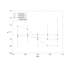
FIG. 1.: The dependence of the ratio $R_{e}$ on $\cos\theta$.

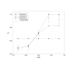
FIG. 2.: The dependence of the ratio $R_{\mu}$ on $\cos\theta$.

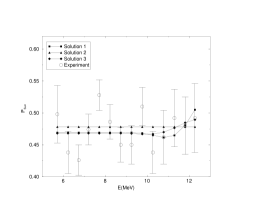
FIG. 3.: The probability $P_{sun}$ as a function of the solar neutrino energy $E$.

FIG. 4.: Stability of Solution 1 with respect to variation of the flux uncertainty factor $\eta$.

FIG. 5.: Stability of Solution 2 with respect to variation of the flux uncertainty factor $\eta$.