Generalized Drell-Hearn-Gerasimov Sum Rule
at Order ${\cal O}(p^{4}$) in Chiral Perturbation Theory

Abstract

We calculate the forward spin-dependent photon-nucleon Compton amplitudes $S_{1}$ and $S_{2}$ as functions of photon energy $\nu$ and mass $Q^{2}$ at the next-to-leading (${\cal O}(p^{4})$) order in chiral perturbation theory, from which we extract the contribution to a generalized Drell-Hearn-Gerasimov sum rule at low $Q^{2}$. The result indicates a much rapid $Q^{2}$ variation of the sum rule than a simple dimensional analysis would yield.

The Drell-Hearn-Gerasimov (DHG) sum rule for the spin-1/2 nucleon relates its anomalous magnetic moment to an integral over the spin-dependent photoproduction cross section[1]. Denoting the energy-dependent total photoproduction cross sections with nucleon spin aligned or anti-aligned with photon helicity as $\sigma_{P}(\nu)$ and $\sigma_{A}(\nu)$, respectively, one may write the DHG sum rule as

$$\int^{\infty}_{\nu_{\rm in}}d\nu{\sigma_{P}(\nu)-\sigma_{A}(\nu)\over\nu}={2\pi^{2}\alpha_{\rm em}\kappa^{2}\over M^{2}}\ ,$$ (1)

where $\kappa$ and $M$ are the anomalous magnetic moment (dimensionless) and mass of the nucleon, respectively, and $\nu_{\rm in}$ is the inelastic threshold. Because of the rapid development of the experimental technology in recent years, it now appears feasible to test the above sum rule which was derived from Low’s low-energy theorem [3] and the assumption of an unsubtracted dispersion relation [1].

On the other hand, polarized electron-nucleon scattering provides a convenient way to measure the spin-dependent virtual-photon production cross section on the nucleon. It is then interesting to explore theoretically if there is a rule that governs the sum (or more precisely, the weighted integral) over the virtual-photon cross section. If such a sum rule exists, it clearly represents a generalization of the Drell-Hearn-Gerasimov sum rule to finite virtual photon mass $Q^{2}$.

In a previous paper by two of us [4], we pointed out that because the DHG sum rule was derived from a dispersion relation for the invariant photon-nucleon Compton amplitude $S_{1}(\nu,Q^{2}=0)$, a generalized sum rule can be naturally constructed from the same dispersion relation at nonzero $Q^{2}$,

$$\int^{\infty}_{\nu_{\rm in}}G_{1}(Q^{2},\nu){d\nu\over\nu}={1\over 4}~{}\overline{S_{1}}(0,Q^{2})\ .$$ (2)

The above sum rule relates the integral of the nucleon spin-dependent structure function $G_{1}(\nu,Q^{2})$ to the Compton amplitude $\overline{S_{1}}(\nu=0,Q^{2})$, where the overline denotes the subtraction of the contribution from the elastic intermediate state. To endow the sum rule with physical content, one needs to find ways to calculate $\overline{S_{1}}(\nu=0,Q^{2})$, extending Low’s low-energy theorem. For the nucleon system at small $Q^{2}$, chiral perturbation theory ($\chi PT$) provides a natural tool. In Ref. [4], we found that $\overline{S_{1}}(\nu=0,Q^{2})$ is independent of $Q^{2}$ at ${\cal O}(p^{3})$. In this letter, we report our result at next-to-leading order, ${\cal O}(p^{4})$.

We first establish our notation and conventions. The forward photon-nucleon Compton scattering tensor is

$$T^{\mu\nu}=i\int d^{4}\xi e^{iq\cdot\xi}\langle PS|{\rm T}J^{\mu}(\xi)J^{\nu}(0)|PS\rangle\ ,$$ (3)

where $|PS\rangle$ is the covariantly-normalized ground state of a nucleon with momentum $P^{\mu}$ and spin polarization $S^{\mu}$. $J_{\mu}=\sum_{i}e_{i}\bar{\psi}_{i}\gamma_{\mu}\psi_{i}$ is the electromagnetic current (with $\psi_{i}$ being the quark field of flavor $i$, and $e_{i}$ its charge in units of the proton charge). The four-vector $q^{\mu}$ is the photon four-momentum. Using Lorentz symmetry, parity and time-reversal invariance, one can express the spin-dependent ($\mu\nu$ antisymmetric) part of $T^{\mu\nu}$ in terms of two scalar functions:

$$T^{[\mu\nu]}(P,q,S)=-i\epsilon^{\mu\nu\alpha\beta}q_{\alpha}\left[S_{\beta}S_{1}(\nu,Q^{2})+\left(\nu\,S_{\beta}-S\cdot q\,P_{\beta}/M\right)S_{2}(\nu,Q^{2})\right]\ ,$$ (4)

where $\epsilon^{0123}=+1$ and $S_{1,2}(\nu,Q^{2})$ are the spin-dependent, invariant Compton amplitudes. Through crossing symmetry, it is easy to see that $S_{1}(\nu,Q^{2})$ is even in $\nu$ and $S_{2}(\nu,Q^{2})$ is odd.

If we restrict ourselves to low $Q^{2}$ and $\nu$, $S_{i}(\nu,Q^{2})$ are low-energy observables and hence it is natural to explore their physical content in chiral perturbation theory, or more broadly in low-energy effective theories. In $\chi$PT, one regards the pion mass $m_{\pi}$ and the external three-momentum $\vec{p}$ small compared to any other scales in the problem. In low-energy effective field theories one also considers expansions in terms of other small parameters, such as the mass difference $\Delta$ between the nucleon and delta resonance. The expansion parameter is then generically denoted as $\epsilon$. In this study, we will ignore the delta resonance effects which seem to be small for $S_{i}(\nu,Q^{2})$ [4].

At order ${\cal O}(p^{3})$, there is no contribution to $\overline{S_{1}}(\nu=0,Q^{2})$ [4]. This conclusion follows from a simple physical fact: the spin-dependent effects on a nonrelativistic particle must vanish as the mass of the particle goes to infinity. Since the nucleon mass $M$ is numerically comparable to $4\pi f_{\pi}$, it is useful to organize $\chi$PT by formally taking the nucleon mass to infinity (heavy-baryon chiral perturbation theory) [5]. From dimensional analysis, the order ${\cal O}(p^{3})$ contribution to $\overline{S_{1}}(\nu=0,Q^{2})$ is independent of $M$ and hence must be zero.

At next-to-leading order, or ${\cal O}(p^{4})$, $\overline{S_{1}}(0,Q^{2})$ is inversely proportional to $M$. To understand the type of Feynman diagrams that we have to consider, it is useful to recall some of the standard infrared power counting in effective field theories as formulated in the heavy-baryon approach. The full lagrangian (including nucleon, delta, photon, and pion fields) can be expanded :

$${\cal L}={\cal L}^{(1)}+{\cal L}^{(2)}+{\cal L}^{(3)}+{\cal L}^{(4)}+...\ ,$$ (5)

where ${\cal L}^{(n)}$ contains terms of order $\epsilon^{n}$, with one power of $\epsilon$ assigned to each derivative, pion mass, photon field, nucleon-delta mass difference, etc. The infrared power of a Feynman diagram is generated from the vertices and the propagators. For polarized Compton scattering, Feynman diagrams start at ${\cal O}(\epsilon^{3})$. For tree diagrams at this order, one needs to consider vertices at ${\cal O}(\epsilon^{n})$ with $n\leq 3$. For one-loop diagrams, however, we need to consider vertices at ${\cal O}(\epsilon)$ only. In general, at order ${\cal O}(\epsilon^{n})$, one needs to consider vertices at order ${\cal O}(\epsilon^{n-2\ell})$ for diagrams of $\ell$-loops. According to the above, we find 20 nonzero Feynman diagrams and their close relatives at ${\cal O}(p^{4})$. These diagrams are shown in Fig. 1, where the cross in each diagram represents an insertion from ${\cal L}^{(2)}$.

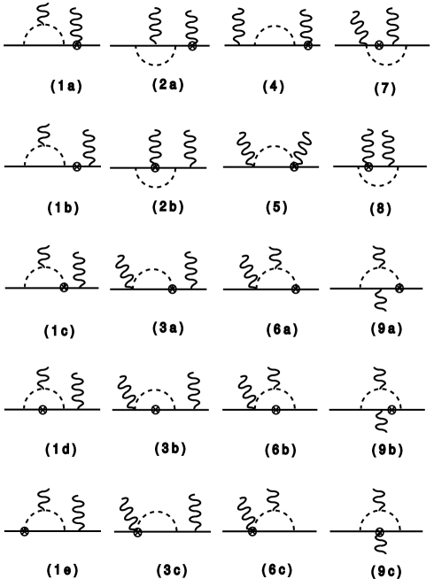
FIG. 1.: The diagrams that contribute to $S_{1,2}(\nu,Q^{2})$ at NLO in heavy baryon $\chi$PT. Obviously, the diagrams from hermiticity and crossing must also be included. The cross indicates an insertion from ${\cal L}^{(2)}$.

We have calculated $S_{1}(\nu,Q^{2})$ as a function of the photon energy $\nu$ and mass $Q^{2}$. The result in the real photon limit was reported in Ref. [6]. Here we are interested in $Q^{2}$ dependence at $\nu=0$,

$$\overline{S_{1}}^{{\cal O}(p^{4})}(0,Q^{2}) = {g_{A}^{2}\pi m_{\pi}\over 8(4\pi f_{\pi})^{2}M}\left[-2(5+6\kappa_{V}+(1+6\kappa_{S})\tau^{3})\right.$$ (8)

$$~{}~{}\left.+\left(4\left(5+6\kappa_{V}+(1+6\kappa_{S})\tau^{3}\right)+{Q^{2}\over m_{\pi}^{2}}\left(3+6\kappa_{V}+(3+10\kappa_{S})\tau^{3}\right)\right)\right.$$

$$~{}~{}\left.\times\,\,\sqrt{m_{\pi}^{2}\over Q^{2}}\sin^{-1}\sqrt{Q^{2}\over 4m_{\pi}^{2}+Q^{2}}\,\,\right],$$

where $\kappa_{S}=-0.120$ and $\kappa_{V}=3.706$ are the experimental values of the isoscalar and isovector anomalous magnetic momentum of the nucleon, respectively, and $\tau^{3}=\pm 1$ for the proton and the neutron, respectively. The above expression vanishes at $Q^{2}=0$ because we have subtracted away the chiral correction to the low-energy theorem [3]. Its slope at $Q^{2}=0$ is

$$\left.{d\overline{S_{1}}(Q^{2})\over dQ^{2}}\right|_{Q^{2}=0}={g_{A}^{2}\pi\over 12(4\pi f_{\pi})^{2}Mm_{\pi}}[(1+3\kappa_{V}+2(1+3\kappa_{S})\tau^{3}].$$ (9)

Following the convention in the literature, we define a dimensionless quantity $\Gamma(Q^{2})\equiv(M^{2}/4)\overline{S_{1}}(Q^{2})$ and write the generalized DHG sum rule as

$$M^{2}\int^{\infty}_{\nu_{\rm in}}G_{1}(\nu,Q^{2})=\Gamma(Q^{2})\ .$$ (10)

Our prediction at small $Q^{2}$ can be expressed as

$$\Gamma^{p}(Q^{2}) = -{\kappa^{2}_{p}\over 4}+6.85~{}Q^{2}({\rm GeV}^{2})+...$$ (11)

$$\Gamma^{n}(Q^{2}) = -{\kappa^{2}_{n}\over 4}+5.54~{}Q^{2}({\rm GeV}^{2})+...\,\,\,\,,$$ (12)

where we have used the low-energy theorem and the result from leading-order chiral perturbation theory. The $Q^{2}$ variation of the generalized DHG sum rule is large, and in fact is about a factor of $\pi^{2}$ larger than what one expects from naive power counting.

For virtual-photon scattering, there is a second sum rule which involves the spin-dependent structure function $G_{2}$ and the Compton amplitude $S_{2}$,

$$\int^{\infty}_{\nu_{\rm in}}{d\nu\over\nu^{2}}G_{2}(\nu,Q^{2})={1\over 4}\overline{S_{2}}^{(1)}(Q^{2})\ ,$$ (13)

where ${\overline{S}_{2}}^{(1)}(Q^{2})\equiv\partial(S_{2}(\nu,Q^{2})-S_{2}^{\rm el}(\nu,Q^{2}))/\partial\nu\,\big{|}_{\nu=0}$ is the slope of the (elastic) subtracted $S_{2}$ at $\nu=0$. In Ref. [4], we have obtained the chiral prediction for $\overline{S_{2}}^{(1)}(Q^{2})$ at leading order. Now we have also the result for $\overline{S_{2}}^{(1)}(Q^{2})$ at next-to-leading order,

$$\overline{S_{2}}^{(1){\cal O}(p^{4})}(Q^{2}) = {g_{A}^{2}\pi m_{\pi}\over 8(4\pi f_{\pi})^{2}M}\left[-2\left(3(5+\tau^{3})+8\left(\kappa_{V}-{Q^{2}\over m_{\pi}^{2}}\right)\right)\right.$$ (16)

$$~{}~{}\left.+\left(12(5+\tau^{3})+32\kappa_{V}+{Q^{2}\over m_{\pi}^{2}}\left(9(1+\tau^{3})+4(3\kappa_{V}+2\kappa_{S}\tau^{3})\right)\right)\right.$$

$$~{}~{}\left.\times\,\,\sqrt{m_{\pi}^{2}\over Q^{2}}\sin^{-1}\sqrt{Q^{2}\over 4m_{\pi}^{2}+Q^{2}}\,\,\right].$$

Numerically, this represents a large correction as one can see below.

In Ref. [7], Bernard, Kaiser, and Meissner suggested to generalize the DHG sum rule using the combiniation ${\overline{S}_{1}}(Q^{2})-Q^{2}{\overline{S}_{2}}^{(1)}(Q^{2})$. Because $\overline{S_{1}}(Q^{2})=0$ at leading order in $\chi$PT, the $Q^{2}$ variation of their sum rule is related entirely to $\overline{S_{2}}^{(1)}(Q^{2})$. Now, up to the next-to-leading order, we find

$${\overline{S}_{1}}(Q^{2})-Q^{2}{\overline{S}_{2}}(Q^{2})=-{\kappa^{2}\over M^{2}}+8{g_{A}^{2}\over(4\pi f_{\pi})^{2}}\left(\sqrt{4m_{\pi}^{2}+Q^{2}\over Q^{2}}\tanh^{-1}\sqrt{Q^{2}\over 4m_{\pi}^{2}+Q^{2}}-1\right)$$ (17)

$$~{}~{}-{g_{A}^{2}\pi m_{\pi}\over 4(4\pi f_{\pi})^{2}M}\left[-2\left(5+\tau^{3}+\kappa_{V}-3\kappa_{S}\tau^{3}-4{Q^{2}\over m_{\pi}^{2}}\right)\right.$$ (18)

$$~{}~{}+\left.\left(4(5+\tau^{3}+\kappa_{V}-3\kappa_{S}\tau^{3})+{Q^{2}\over m_{\pi}^{2}}(3+3\kappa_{V}+3\tau^{3}-\kappa_{S}\tau^{3})\right)\sqrt{m_{\pi}^{2}\over Q^{2}}\sin^{-1}\sqrt{Q^{2}\over 4m_{\pi}^{2}+Q^{2}}\,\,\right]$$ (19)

$$~{}~{}+{\cal O}(p^{5})\ .$$ (20)

The slope at small $Q^{2}$ is

$$\left.{d({\overline{S}_{1}}(Q^{2})-Q^{2}{\overline{S}_{2}^{(1)}}(Q^{2}))\over dQ^{2}}\right|_{Q^{2}=0}=\left({g_{A}\over 4\pi m_{\pi}f_{\pi}}\right)^{2}\left[{2\over 3}-{\pi\over 6}{m_{\pi}\over M}(13+2\tau^{3}+2\kappa_{V})\right].$$ (21)

The first term in the brackets was first obtained in Ref. [7] and, as we have stated, comes from the leading order $\overline{S_{2}}^{(1)}(Q^{2})$. The subleading correction is our new result. Because of the large coefficient, $13+2\kappa_{V}\sim 20.4$, the ${\cal O}(p^{4})$ contribution is about a factor of 2 larger than the leading contribution, and has the opposite sign. As in the case of the spin polarizability [6], we question the validity of the chiral expansion of this quantity.

To conclude, we have calculated the ${\cal O}(p^{4})$ correction to the generalized DHG sum rules. In a natural scheme introduced in Ref. [4], the $Q^{2}$ dependence of the generalized sum rule is much larger than expected from a naive dimensional analysis. The same phenomenon is presumably responsible for an overwhelming next-to-leading-order correction to the rule considered by Bernard, Kaiser, and Meissner [7].

REFERENCES

• [1] S. D. Drell and A. C. Hearn, Phys. Rev. Lett. 16 908 (1966);
S. B. Gerasimov, Sov. J. Nucl. Phys. 2 430 (1966).
• [2] A. M. Bernstein and B. R. Holstein, Proceedings on Chiral Dynamics: Theory and Experiment (Cambridge, MA, 1994).
• [3] F. Low, Phys. Rev. 96, 1428 (1954); Phys. Rev. 110, 974 (1958).
• [4] X. Ji and J. Osborne, hep-ph/9905410.
• [5] E. Jenkins and A. V. Manohar, Phys. Lett. B255 558 (1991).
• [6] X. Ji, C.W. Kao, and J. Osborne, hep-ph/9908526.
• [7] V. Bernard, N. Kaiser, and Ulf-G. Meissner, Phys. Rev. D 48, 3062 (1993).