CERN-TH/99-306

MC-TH-99-14

October 1999

Predicting $F_{2}^{D(3)}$ from the dipole cross-section

J.ย R.ย Forshaw***Theory Division, CERN, 1211 Geneva 23, Switzerland., G.ย R.ย Kerley and G.ย Shawa

aTheoretical Physics Group, Department of Physics and Astronomy,
The University of Manchester, M13 9PL, UK

Abstract

We employ a parameterisation of the proton dipole cross section previously extracted from electroproduction and photoproduction data to predict the diffractive structure function $F_{2}^{D(3)}(Q^{2},\beta,x_{I\!\!P})$. Comparison with HERA H1 data yields good agreement.

1 Introduction

The proton dipole cross section $\sigma_{d}$ย is a universal quantity in singly dissociative diffractive $\gamma$ p processes.ย [1, 2] It is simply the total cross section for scattering a qqฬ„ pair of a given size and energy in the photonic fluctuation off the proton target. We make use of a parameterisation used to extract $\sigma_{d}$ย from a fit to electroproduction and photoproduction $\gamma$ p total cross-section dataย [3] to predict the diffractive structure function $F_{2}^{D(3)}(Q^{2},\beta,x_{I\!\!P})$.

Refer to caption
Figure 1: The dipole fluctuation of the incoming photon.

2 Functional forms

The dipole cross-section is in general a function of three variables (Figureย 1): s=W2๐‘ superscript๐‘Š2s=W^{2}, the CMS energy squared of the photon proton system; $r$, the transverse separation averaged over all orientations of the qqฬ„ pair; and $\alpha$, the fraction of the incoming photon light cone energy possessed by one member of the qqฬ„ pair. We assumed a form with two terms, each with a Regge type s๐‘ s dependence and no dependence on $\alpha$. Specifically, we assumed

ฯƒdโ€‹(s,r)=a0Sโ€‹(1โˆ’11+(a1Sโ€‹r+a2Sโ€‹r2)2)โ€‹(r2โ€‹s)ฮปS+(a1Hโ€‹r+a2Hโ€‹r2+a3Hโ€‹r3)2โ€‹expโก(โˆ’ฮฝH2โ€‹r)โ€‹(r2โ€‹s)ฮปH.subscript๐œŽ๐‘‘๐‘ ๐‘Ÿsuperscriptsubscript๐‘Ž0๐‘†111superscriptsuperscriptsubscript๐‘Ž1๐‘†๐‘Ÿsuperscriptsubscript๐‘Ž2๐‘†superscript๐‘Ÿ22superscriptsuperscript๐‘Ÿ2๐‘ subscript๐œ†๐‘†superscriptsuperscriptsubscript๐‘Ž1๐ป๐‘Ÿsuperscriptsubscript๐‘Ž2๐ปsuperscript๐‘Ÿ2superscriptsubscript๐‘Ž3๐ปsuperscript๐‘Ÿ32superscriptsubscript๐œˆ๐ป2๐‘Ÿsuperscriptsuperscript๐‘Ÿ2๐‘ subscript๐œ†๐ป\sigma_{d}(s,r)=a_{0}^{S}\left(1-\frac{1}{1+(a_{1}^{S}r+a_{2}^{S}r^{2})^{2}}\right)(r^{2}s)^{\lambda_{S}}+(a_{1}^{H}r+a_{2}^{H}r^{2}+a_{3}^{H}r^{3})^{2}\exp(-\nu_{H}^{2}r)(r^{2}s)^{\lambda_{H}}. (1)

The dipole cross section is related to the photon proton cross section via

ฯƒฮณโˆ—,pL,T=โˆซdโ€‹ฮฑโ€‹d2โ€‹rโ€‹|ฯˆฮณL,Tโ€‹(ฮฑ,r)|2โ€‹ฯƒdโ€‹(s,r,ฮฑ)subscriptsuperscript๐œŽ๐ฟ๐‘‡superscript๐›พ๐‘d๐›ผsuperscriptd2๐‘Ÿsuperscriptsuperscriptsubscript๐œ“๐›พ๐ฟ๐‘‡๐›ผ๐‘Ÿ2subscript๐œŽ๐‘‘๐‘ ๐‘Ÿ๐›ผ\sigma^{L,T}_{\gamma^{*},p}=\int\mbox{d}\alpha\mbox{d}^{2}r\ |\psi_{\gamma}^{L,T}(\alpha,r)|^{2}\sigma_{d}(s,r,\alpha) (2)

where $\psi_{\gamma}^{L,T}(\alpha,r)$ are the longitudinal and transverse components of the light cone photon wave function. For the photon wave function itself, we used the tree level QED expressionย [1, 4] modified by a factor $f(r)$ to represent confinement effects:

$\displaystyle|\psi_{L}(\alpha,r)|^{2}$ $\displaystyle=$ $\displaystyle\frac{6}{\pi^{2}}\alpha_{em}\sum_{q=1}^{3}e_{q}^{2}Q^{2}\alpha^{2}(1-\alpha)^{2}K_{0}^{2}(\epsilon r)\times f(r)$ (3)
$\displaystyle|\psi_{T}(\alpha,r)|^{2}$ $\displaystyle=$ $\displaystyle\frac{3}{2\pi^{2}}\alpha_{em}\sum_{q=1}^{3}e_{q}^{2}\left\{[\alpha^{2}+(1-\alpha)^{2}]\epsilon^{2}K_{1}^{2}(\epsilon r)+m_{f}^{2}K_{0}^{2}(\epsilon r)\right\}\times f(r)$ (4)

and

$$f(r)=\frac{1+B\exp(-c^{2}(r-R)^{2})}{1+B\exp(-c^{2}R^{2})}.$$ (5)

Here $\epsilon^{2}=\alpha(1-\alpha)Q^{2}+m_{f}^{2}\;,$ $K_{0}$ and $K_{1}$ are modified Bessel functions and the sum is over 3 light quark flavours, with a generic mass of assumed value $m_{f}^{2}=0.08$ GeV2. The values of the constants $B$, $c^{2}$, and $R$ were generated by the fit.

3 Calculating $F_{2}^{D(3)}$

Refer to caption
Refer to caption
Figure 2: The qqฬ„ and qqฬ„g contributions to $F_{2}^{D(3)}$.

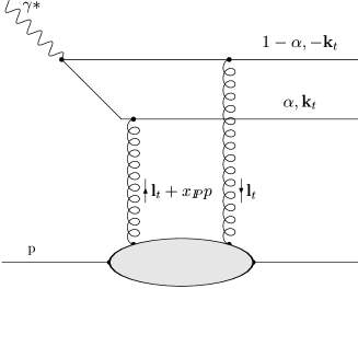
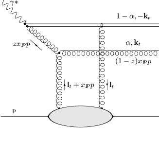
To calculate the contribution of the quark antiquark dipole to $F_{2}^{D(3)}$ we made use of expressions derived from a momentum space treatmentย [5, 6]. Also, we calculated the contribution of the higher qqฬ„g Fock state using an effective two gluon dipole description from the same source. Typical Feynman diagrams are shown in Figureย 2. For compatibility with this approach, we must replace s๐‘ s by s~~๐‘ \tilde{s}, where s~=Q2โ€‹(1/xIโ€‹Pโˆ’1)~๐‘ superscript๐‘„21subscript๐‘ฅ๐ผ๐‘ƒ1\tilde{s}=Q^{2}(1/x_{I\!\!P}-1). First defining

ฮฆ0,1โ‰กโˆซ0โˆžrโ€‹dโ€‹rโ€‹K0,1โ€‹(ฯตโ€‹r)โ€‹ฯƒdโ€‹(r,s~)โ€‹J0,1โ€‹(kโ€‹r)โ€‹โˆซ0โˆžrโ€‹dโ€‹rโ€‹fโ€‹(r)โ€‹K0,1โ€‹(ฯตโ€‹r)โ€‹ฯƒdโ€‹(r,s~)โ€‹J0,1โ€‹(kโ€‹r),subscriptฮฆ01superscriptsubscript0๐‘Ÿd๐‘Ÿsubscript๐พ01italic-ฯต๐‘Ÿsubscript๐œŽ๐‘‘๐‘Ÿ~๐‘ subscript๐ฝ01๐‘˜๐‘Ÿsuperscriptsubscript0๐‘Ÿd๐‘Ÿ๐‘“๐‘Ÿsubscript๐พ01italic-ฯต๐‘Ÿsubscript๐œŽ๐‘‘๐‘Ÿ~๐‘ subscript๐ฝ01๐‘˜๐‘Ÿ\Phi_{0,1}\equiv\int_{0}^{\infty}r\mbox{d}rK_{0,1}(\epsilon r)\sigma_{d}(r,\tilde{s})J_{0,1}(kr)\int_{0}^{\infty}r\mbox{d}rf(r)K_{0,1}(\epsilon r)\sigma_{d}(r,\tilde{s})J_{0,1}(kr), (6)

we have for the longitudinal and transverse qqฬ„ components respectively

$$x_{I\!\!P}F^{D}_{q\bar{q},L}(Q^{2},\beta,x_{I\!\!P})=\frac{3Q^{6}}{32\pi^{4}\beta b}\cdot\sum_{f=1}^{3}e_{f}^{2}\cdot 2\int_{\alpha_{0}}^{1/2}\mbox{d}\alpha\alpha^{3}(1-\alpha)^{3}\Phi_{0}$$ (7)
$$x_{I\!\!P}F^{D}_{q\bar{q},T}(Q^{2},\beta,x_{I\!\!P})=\frac{3Q^{4}}{128\pi^{4}\beta b}\cdot\sum_{f=1}^{3}e_{f}^{2}\cdot 2\int_{\alpha_{0}}^{1/2}\mbox{d}\alpha\alpha(1-\alpha)\left\{\epsilon^{2}[\alpha^{2}+(1-\alpha)^{2}]\Phi_{1}+m^{2}\Phi_{0}\right\}$$ (8)

where the lower limit of the integral over $\alpha$ is given by $\alpha_{0}=(1/2)\left(1-\sqrt{1-4m_{f}^{2}/M_{X}^{2}}\right)$ and $b$ is the slope parameter, which we have taken as 7.2ย [7]. For the qqฬ„g term we have

$\displaystyle x_{I\!\!P}F^{D}_{q\bar{q}g}(Q^{2},\beta,x_{I\!\!P})=\frac{81\beta\alpha_{S}}{512\pi^{5}b}\sum_{f}e_{f}^{2}\int_{\beta}^{1}\frac{\mbox{d}z}{(1-z)^{3}}\left[\left(1-\frac{\beta}{z}\right)^{2}+\left(\frac{\beta}{z}\right)^{2}\right]$ (9)
$\displaystyle\times$ โˆซ0(1โˆ’z)โ€‹Q2dโ€‹kt2โ€‹lnโก((1โˆ’z)โ€‹Q2kt2)โ€‹[โˆซ0โˆžuโ€‹dโ€‹uโ€‹ฯƒdโ€‹(u/kt,s~)โ€‹K2โ€‹(z1โˆ’zโ€‹u2)โ€‹J2โ€‹(u)]2superscriptsubscript01๐‘งsuperscript๐‘„2dsuperscriptsubscript๐‘˜๐‘ก21๐‘งsuperscript๐‘„2superscriptsubscript๐‘˜๐‘ก2superscriptdelimited-[]superscriptsubscript0๐‘ขd๐‘ขsubscript๐œŽ๐‘‘๐‘ขsubscript๐‘˜๐‘ก~๐‘ subscript๐พ2๐‘ง1๐‘งsuperscript๐‘ข2subscript๐ฝ2๐‘ข2\displaystyle\int_{0}^{(1-z)Q^{2}}\mbox{d}k_{t}^{2}\ln\left(\frac{(1-z)Q^{2}}{k_{t}^{2}}\right)\left[\int_{0}^{\infty}u\mbox{d}u\;\sigma_{d}(u/k_{t},\tilde{s})K_{2}\left(\sqrt{\frac{z}{1-z}u^{2}}\right)J_{2}(u)\right]^{2} (10)

with $\alpha_{S}=0.2$. (We have inserted a missing factor of 1/2 compared with the expression inย [6].) This expression diverges if our parameterisation is used as it stands. However, this is due solely to the mild divergence after $\sigma_{d}$ย saturates in $r$ of the factor (r2โ€‹s)ฮปSsuperscriptsuperscript๐‘Ÿ2๐‘ subscript๐œ†๐‘†(r^{2}s)^{\lambda_{S}} as $r\rightarrow\infty$. This behaviour at large $r$ is not determined by data and is an artefact of the parameterisation. Hence we have imposed a saturation value for $\sigma_{d}$ย of its value at $r$ = 2ย fm for all higher $r$. Plots of the contributions to $x_{I\!\!P}F_{2}^{D(3)}$ calculated from these expressions are compared with H1 1994 dataย [8] in Figureย 3.

Refer to caption
Figure 3: Contributions to $x_{I\!\!P}F_{2}^{D(3)}$ compared with H1 1994 data. Full, dotted, dashed and dot dashed lines are the total, longitudinal qqฬ„, transverse qqฬ„ and qqฬ„g contributions respectively.

Agreement is good, even at low $\beta$ where the qqฬ„g term dominates. Comparison with ZEUS 1994 dataย [9] also gives good agreement overall but with deviations at larger $Q^{2}$ย values for small and moderate $\beta$.

4 Conclusions

We have successfully predicted the diffractive structure function $F_{2}^{D(3)}$using a parameterised dipole cross section obtained from electro- and photoproduction data. Unlike the model proposed inย [6, 10], the parameterisation exhibits effective saturation in $r$ only, with no saturation in the energy variable s=W2๐‘ superscript๐‘Š2s=W^{2}. Agreement with data is reasonable, leading to the conclusion that the HERA data do not necessarily indicate such saturation at present energies.

5 Acknowledgements

GRK would like to thank PPARC for a Studentship. This work was supported in part by the EU Fourth Programme โ€˜Training and Mobility of Researchersโ€™, Network โ€˜Quantum Chromodynamics and the Deep Structure of Elementary Particlesโ€™, contract FMRX-CT98-0194 (DG 12-MIHT).

References

  • [1] N.N.ย Nikolaev and B.G.ย Zakharov, Z. Phys. C49 (1991) 607
  • [2] N.N.ย Nikolaev and B.G.ย Zakharov, Z. Phys. C53 (1992) 331
  • [3] J.R.ย Forshaw, G.ย Kerley and G.ย Shaw, Phys. Rev. D60 (1999) 074012, hep-ph/9903341
  • [4] H.G.ย Dosch, T.ย Gousset, G.ย Kulzinger and H.J.ย Pirner, Phys. Rev. D55 (1997) 2602, hep-ph/9608203
  • [5] M.ย Wรผsthoff, Phys. Rev. D56 (1997) 4311, hep-ph/9702201
  • [6] K.ย Golec-Biernat and M.ย Wรผsthoff, Phys. Rev. D60 (1999) 114023, hep-ph/9903358
  • [7] J.ย Breitweg et al, ZEUS Collab., Eur. Phys. J. C1 (1998) 81, hep-ex/9709021
  • [8] C.ย Adloff et al., H1 Collab., Zeit. Phys. C76 (1997) 613, hep-ex/9708016
  • [9] J.ย Breitweg et al., ZEUS Collab., Eur. Phys. J. C6 (1999) 43, hep-ex/9807010
  • [10] K.ย Golec-Biernat and M.ย Wรผsthoff, Phys. Rev. D59 (1999) 014017, hep-ph/9807513