Neutrino Anomalies without Oscillations

Abstract

I review explanations for the three neutrino anomalies (solar, atmospheric and LSND) which go beyond the “conventional” neutrino oscillations induced by mass-mixing. Several of these require non-zero neutrino masses as well.

I Introduction

As is well-known, it is not possible to account for all three neutrino anomalies with just the three known neutrinos $(\nu_{e},\nu_{\mu}$ and $\nu_{\tau})$. If one or more of them can be explained in some other way, then no extra sterile neutrinos need be invoked. This is one motivation for exotic scenarios. In any case it is important to rule out all explanations other than oscillations in order to establish neutrino mixing and oscillations as the unique explanation for the three observed neutrino anomalies.

I should mention that, in general, some (but not all) non-oscillatory explanations of the neutrino anomalies will involve non-zero neutrino masses and mixings. Therefore, they tend to be neither elegant nor economical. But the main issue here is whether we can establish oscillations unequivocally and uniquely as the cause for the observed anomalies.

I first summarize some of the exotic scenarios and then consider each anomaly in turn.

II Mixing and Oscillations of massless $\nu^{\prime}s$

There are three different ways that massless neutrinos may mix and even oscillate. These are as follows.

1. If flavor states are mixtures of massless as well massive states, then when they are produced in reactions with Q-values smaller than the massive state; the flavor states are massless but not orthogonal[1]. For example, if $\quad\nu_{e}=\sum_{i=1}^{4}U_{ei}\nu_{i}$, $\nu_{\mu}=\sum_{i=1}^{4}U_{\mu i}\nu_{i}$ and $m_{i}=0$ for $i=1$ to 3 but $m_{4}$ = 50 GeV; then “$\nu_{e}$” produced in $\beta$-decay and “$\nu_{\mu}$” produced in $\pi$-decay are massless but not orthogonal and

$$\left<\nu_{e}\mid\nu_{\mu}\right>=-U_{e4}^{*}\ U_{\mu 4}$$ (1)

On the other hand $\nu_{e}$ and $\nu_{\mu}$ produced in $W$ decay will be not massless and will be more nearly orthogonal. Hence, the definition of flavor eigenstate is energy and reaction dependent and not fundamental. Current limits[2] on orthogonality of $\nu_{e},\nu_{\mu}$ and $\nu_{\tau}$ make it impossible for this to play any role in the current neutrino anomalies.

2. When Flavor Changing Neutral Currents as well as Non-Universal Neutral Current Couplings of neutrinos exist, for example:

$$\epsilon_{q}\frac{4G_{F}}{\sqrt{2}}\left\{\bar{\nu}_{el}\ \gamma_{\mu}\ \nu{{}_{\tau_{L}}}\bar{q}_{L}\ \gamma_{\mu}q_{L}\ \ +h.c.\right\}$$ (2)

$$+ \epsilon^{\prime}_{q}\frac{4G_{F}}{\sqrt{2}}\ \left\{\bar{\nu}_{eL}\ \gamma_{\mu}\ \nu{{}_{e_{L}}}-\bar{\nu}_{\tau L}\gamma_{\mu}\ \nu_{\tau L}\right\}\left\{\bar{q}_{L}\ \gamma_{\mu}\ q_{L}\right\}$$ (3)

Such couplings arise in R-parity violating supersymmetric theories[3]. In general, in these theories, one expects neutrino masses at some level here it is assumed that the FCNC provides the dominant effect. In this case the propagation of $\nu_{e}$ and $\nu_{\tau}$ in matter is described by the equation:

$$i\frac{d}{dt}\left(\begin{array}[]{c}\nu_{e}\\ \nu_{\tau}\end{array}\right)_{L}=\left(\begin{array}[]{cc}\alpha+\beta&\gamma\\ \gamma&-\beta\end{array}\right)\left(\begin{array}[]{c}\nu_{e}\\ \nu_{\tau}\end{array}\right)_{L}$$ (10)

where $\alpha=G_{F}N_{e},\beta=\epsilon_{q}G_{F}N_{q}$ and $\gamma=\epsilon^{\prime}_{q}G_{F}N_{q}$. There is a resonance at $\alpha+2\beta=0$ or $\epsilon_{q}=-\frac{1}{2}N_{e}/N_{q}$ and $\nu_{e}$ can convert to $\nu_{\tau}$ completely. This matter effect which effectively mixes flavors in absence of masses was first pointed out by Wolfenstein in the same paper[4] where matter effects were first discussed. The resonant conversion is just like in the conventional MSW effect, except that there is no energy dependence and $\nu$ and $\bar{\nu}$ are affected the same way. This possibility has been discussed in connection with both solar and atmospheric anomalies.

3. (a) Flavor violating Gravity wherein it is proposed that gravitational couplings of neutrinos are flavor non-diagonal[5] and equivalence principle is violated. For example, $\nu_{1}$ and $\nu_{2}$ may couple to gravity with different strengths:

$$H_{gr}=f_{1}GE\phi+f_{2}GE\phi$$ (11)

where $\phi$ is the gravitational potential. Then if $\nu_{e}$ and $\nu_{\mu}$ are mixtures of $\nu_{1}$ and $\nu_{2}$ with a mixing angle $\theta$, oscillations will occur with a flavor survival probability

$$P=1-sin^{2}2\theta sin^{2}(\frac{1}{2}\delta f\phi EL)$$ (12)

when $\phi$ is constant over the distance L and $\delta f=f_{1}-f_{2}$ is the small deviation from universality of gravitational coupling. Equivalence principle is also violated.

(b) Another possibility is violation of Lorentz invariance[6] wherein all particles have their own maximum attainable velocities (MAV) which are all different and in general also different from speed of light: then if $\nu_{1}$ and $\nu_{2}$ are MAV eigenstates with MAV’s $v_{1}$ and $v_{2}$ and $\nu_{e}$ and $\nu_{\mu}$ are mixtures of $\nu_{1}$ and $\nu_{2}$ with mixing angle $\theta$, the survival probability of a given flavor is

$$P=1-sin^{2}2\theta\ sin^{2}\left(\frac{1}{2}\delta vEL\right)$$ (13)

where $\delta v=v_{1}-v_{2}$.

As far as neutrino oscillations are concerned, these two cases are identical in their dependence on LE instead of L/E as in the conventional oscillations[7].

III Neutrino Decay

Neutrino decay[8] implies a non-zero mass difference between two neutrino states and thus, in general, mixing as well. I will consider here only non-radiative decays. We assume a component of $\nu_{\alpha},$ i.e., $\nu_{2}$, to be the only unstable state, with a rest-frame lifetime $\tau_{0}$, and we assume two flavor mixing, for simplicity:

$$\nu_{\mu}=cos\theta\nu_{2}\ +sin\theta\nu_{1}$$ (14)

with $m_{2}>m_{1}$. From Eq. (2) with an unstable $\nu_{2}$, the $\nu_{\alpha}$ survival probability is

$$P_{\alpha\alpha} = sin^{4}\theta\ +cos^{4}\theta{\rm exp}(-\alpha L/E)$$ (15)

$$+ 2sin^{2}\theta cos^{2}\theta{\rm exp}(-\alpha L/2E)cos(\delta m^{2}L/2E),$$ (16)

where $\delta m^{2}=m^{2}_{2}-m_{1}^{2}$ and $\alpha=m_{2}/\tau_{0}$. Since we are attempting to explain neutrino data without oscillations there are two appropriate limits of interest. One is when the $\delta m^{2}$ is so large that the cosine term averages to 0. Then the survival probability becomes

$$P_{\mu\mu}=sin^{4}\theta\ +cos^{4}\theta{\rm exp}(-\alpha L/E)$$ (17)

Let this be called decay scenario A. The other possibility is when $\delta m^{2}$ is so small that the cosine term is 1, leading to a survival probability of

$$P_{\mu\mu}=(sin^{2}\theta+cos^{2}\theta{\rm exp}(-\alpha L/2E))^{2}$$ (18)

corresponding to decay scenario B. Decay models for both kinds of scenarios can be constructed; although they require fine tuning and are not particularly elegant.

IV LSND

In the LSND experiment, what is observed is the following[9]. In the decay at rest (DAR) which is $\mu^{+}\rightarrow e^{+}\nu_{e}\bar{\nu}_{\mu}$ which should give a pure $\nu_{e}$ signal, there is a flux of $\bar{\nu_{e}^{\prime}s}$ at a level of about $3.10^{-3}$ of the $\nu_{e}^{\prime}s$. (There is a similar signal for $\nu^{\prime}_{e}s$ accompanying $\bar{\nu}^{\prime}_{e}s$ in the decay in flight of $\mu^{-}\rightarrow e^{-}\bar{\nu}_{e}\nu_{\mu})$. Now this could be accounted for without oscillations[10] provided that the conventional decay mode $\mu^{+}\rightarrow e^{+}\nu_{e}\bar{\nu}_{\mu}(\mu^{-}\rightarrow e^{-}\bar{\nu}_{e}\nu_{\mu})$ is accompanied by the rare mode $\mu^{+}\rightarrow e^{+}\bar{\nu}_{e}{\rm X}\ (\mu^{-}\rightarrow e^{-}\nu_{e}\bar{\rm X})$ at a level of branching fraction of $3.10^{-3}$. Assuming X to be a single particle, what can X be? It is straight forward to rule out X as being (i) $\nu_{\mu}$ (too large a rate for Muonium-Antimuonium transition rate), (ii) $\nu_{e}$ (too large a rate for FCNC decays of $Z$ such as $Z\rightarrow\mu\bar{e}+\bar{\mu}e)$ and (iii) $\nu_{\tau}$ (too large a rate for FCNC decays of $\tau$ such as $\tau\rightarrow\mu ee)$.

The remaining possibilities for X are $\bar{\nu}_{\alpha}$ or $\nu_{\rm{sterile}}$. No simple models exist which lead to such decays. Rather Baroque models can be constructed which involve a large number of new particles[11].

Experimental tests to distinguish this rare decay possibility from the conventional oscillation explanation are easy to state. In the rare decay case, the rate is constant and shows no dependence on L or E.

One can also ask whether the $\bar{\nu}_{e}$ events seen in LSND could have been caused by new physics at the detector; for example a small rate for the “forbidden” reaction $\bar{\nu}_{\mu}+p\rightarrow n+e^{+}$. This is ruled out, since a fractional rate of $3.10^{-3}$ for this reaction, leads (via crossing) to a rate for the decay mode $\pi^{+}\rightarrow e^{+}\nu_{\mu}$ in excess of known bounds.

V Solar Neutrinos

Oscillations of massless neutrinos via Flavor Changing Neutral Currents (FCNC) and Non Universal Neutral Currents (NUNC) in matter have been considered[3, 12] as explanation for the solar neutrino observations, most recently by Babu, Grossman and Krastev[13]. Using the most recent data from Homestake, SAGE, GALLEX and Super-Kamiokande, they find good fits with $\epsilon_{u}\sim 10^{-2}$ and $\epsilon^{\prime}_{u}\sim 0.43$ or $\epsilon_{d}\sim$ 0.1 to 0.01 with $\epsilon^{\prime}_{d}\sim 0.57$.

Since the matter effect in this case is energy independent, the explanation for different suppression for ${}^{8}B$, ${}^{7}Be$ and pp neutrinos as inferred is interesting. The differing suppression arises from the fact the production region for each of these neutrinos differ in electron and nuclear densities. This solution resembles the large angle MSW solution with the difference that the day-night effect is energy-independent.

The massless neutrino oscillations described in Eq.(6) also offer a possible solution to solar neutrino observations. There are three solutions. Two are characterized by $\sin^{2}2\theta\sim 2.10^{-3},\delta v/2\sim 6.10^{-19}$ and $\sin^{2}2\theta\sim 0.7,\delta v/2\sim 10^{-21}$; these are analogs of the small angle MSW and large angle MSW solutions[14]. These are now ruled out[15] (for both $\nu_{e}-\nu_{\mu}$ and $\nu_{e}-\nu_{\tau})$ by the recent NUTEV data[16]. The third one at $\sin^{2}2\theta\sim 1$ and $\frac{\delta v}{2}\sim 10^{-24}$ (the analog of the vacuum solution) is the only one allowed[17]. This possibility can be tested in Long Baseline experiments.

The possibility of solar neutrinos decaying to explain the discrepancy is a very old suggestion[18]. The most recent analysis of the current solar neutrino data finds that no good fit can be found: $U_{ei}\approx 0.6$ and $\tau_{\nu}$ (E=10 MeV) $\sim 6$ to 27 sec. come closest[19]. The fits become acceptable only if the suppression of the solar neutrinos is energy independent as proposed by several authors[20] (which is possible if the Homestake data are excluded from the fit). The above conclusions are valid for both the decay scenarios A as well as B.

VI Atmospheric Neutrinos

The massless FCNC scenario has been recently considered for the atmospheric neutrinos by Gonzales-Garcia et al.[21] with the matter effect supplied by the earth. Good fits were found for the partially contained and multi-GeV events with $\epsilon_{q}\sim 1,\epsilon^{\prime}_{q}\sim 0.02$ as well $\epsilon_{q}\sim 0.08,\epsilon_{q}^{\prime}\sim 0.07$. The fit is poorer when higher energy events corresponding to up-coming muons are included[22, 23]. The expectations for future LBL experiments are quite distinctive: for MINOS, one expects $P_{\mu\mu}\sim 0.1$ and $P_{\mu\tau}\sim 0.9.$ The story for massless neutrinos oscillating via violation of Equivalence Principle or Lorentz Invariance is very similar. Assuming large $\nu_{\mu}-\nu_{\tau}$ mixing, and $\delta v/2\sim 2.10^{-22},$ a good fit to the contained events can be obtained[24]; but as soon as multi-GeV and thrugoing muon events are included, the fit is quite poor[22, 23].

Turning to neutrino decay scenario A, it was found that it is possible to choose $\theta$ and $\alpha$ to provide a good fit to the Super-Kamiokande L/E distributions of $\nu_{\mu}$ events and $\nu_{\mu}/\nu_{e}$ event ratio[25]. The best-fit values of the two parameters are $cos^{2}\theta\sim 0.87$ and $\alpha\sim 1GeV/D_{E},$ where $D_{E}=12800$ km is the diameter of the Earth. This best-fit $\alpha$ value corresponds to a rest-frame $\nu_{2}$ lifetime of

$$\tau_{0}=m_{2}/\alpha\sim\frac{m_{2}}{(1eV)}\times 10^{-10}s.$$ (19)

However, it was then shown that the fit to the higher energy events in Super-K (especially the upcoming muons) is quite poor[22, 23].

In all these three cases, the reason that the inclusion of high energy upcoming muon events makes the fits poorer is very simple. The upcoming muons come from much higher energy $\nu_{\mu}^{\prime}s$ and although there is some suppression, it is less than what is observed for lower energy events at the same L (zenith angle). This is in accordance with expectations from conventional oscillations. The energy dependence in the above three scenarios is different and fails to account for the data. In the FCNC case there is no energy dependence and so the high energy $\nu_{\mu}^{\prime}s$ should have been equally depleted, in the FV Gravity (or Lorentz invariance violation) at high energies the oscillations should average out to give uniform 50% suppression and in the decay A scenario due to time dilation the decay is suppressed and there is hardly any depletion of $\nu_{\mu}^{\prime}s$.

Turning to decay scenario B, consider the following possibility[26]. The three weak coupling states $\nu_{\mu},\nu_{\tau},\nu_{s}$ (where $\nu_{s}$ is a sterile neutrino) may be related to the mass eigenstates $\nu_{2}\nu_{3}\nu_{4}$ by the approximate mixing matrix.

$$\left(\begin{array}[]{c}\nu_{\mu}\\ \nu_{\tau}\\ \nu_{s}\end{array}\right)=\left(\begin{array}[]{ccc}\cos\theta&\sin\theta&0\\ -\sin\theta&\cos\theta&0\\ 0&0&1\end{array}\right)\left(\begin{array}[]{c}\nu_{2}\\ \nu_{3}\\ \nu_{4}\end{array}\right)$$ (20)

and the decay is $\nu_{2}\to\bar{\nu}_{4}+J$. The electron neutrino, which we identify with $\nu_{1}$, cannot mix very much with the other three because of the more stringent bounds on its couplings[27], and thus our preferred solution for solar neutrinos would be small angle matter oscillations.

Then the $\delta m_{23}^{2}$ in Eq. (1) is not related to the $\delta m_{24}^{2}$ in the decay, and can be very small, say $<10^{-4}\rm\,eV^{2}$ (to ensure that oscillations play no role in the atmospheric neutrinos). In that case, the oscillating term is 1 and $P(\nu_{\mu}\to\nu_{\mu})$ becomes

$$P(\nu_{\mu}\to\nu_{\mu})=(\sin^{2}\theta+\cos^{2}\theta e^{-\alpha L/2E})^{2}$$ (21)

This is identical to Eq. (13) in Ref. [8].

In order to compare the predictions of this model with the standard $\nu_{\mu}\leftrightarrow\nu_{\tau}$ oscillation model, we have calculated with Monte Carlo methods the event rates for contained, semi-contained and upward-going (passing and stopping) muons in the Super-K detector, in the absence of ‘new physics’, and modifying the muon neutrino flux according to the decay or oscillation probabilities discussed above. We have then compared our predictions with the SuperK data [25], calculating a $\chi^{2}$ to quantify the agreement (or disagreement) between data and calculations. In performing our fit (see Ref. [22] for details) we do not take into account any systematic uncertainty, but we allow the absolute flux normalization to vary as a free parameter $\beta$.

The ‘no new physics model’ gives a very poor fit to the data with $\chi^{2}=281$ for 34 d.o.f. (35 bins and one free parameter, $\beta$). For the standard $\nu_{\mu}\leftrightarrow\nu_{\tau}$ oscillation scenario the best fit has $\chi^{2}=33.3$ (32 d.o.f.) and the values of the relevant parameters are $\Delta m^{2}=3.2\times 10^{-3}$ eV², $\sin^{2}2\theta=1$ and $\beta=1.15$. This result is in good agreement with the detailed fit performed by the SuperK collaboration [25] giving us confidence that our simplified treatment of detector acceptances and systematic uncertainties is reasonable. The decay model of Equations (3) and (4) above gives an equally good fit with a minimum $\chi^{2}=33.7$ (32 d.o.f.) for the choice of parameters

$$\tau_{\nu}/m_{\nu}=63\rm~{}km/GeV,\ \cos^{2}\theta=0.30$$ (22)

and normalization $\beta=1.17$.

In Fig. 1 we compare the best fits of the two models considered (oscillations and decay) with the SuperK data. In the figure we show (as data points with statistical error bars) the ratios between the SuperK data and the Monte Carlo predictions calculated in the absence of oscillations or other form of ‘new physics’ beyond the standard model. In the six panels we show separately the data on $e$-like and $\mu$-like events in the sub-GeV and multi-GeV samples, and on stopping and passing upward-going muon events. The solid (dashed) histograms correspond to the best fits for the decay model ($\nu_{\mu}\leftrightarrow\nu_{\tau}$ oscillations). One can see that the best fits of the two models are of comparable quality. The reason for the similarity of the results obtained in the two models can be understood by looking at Fig. 2, where we show the survival probability $P(\nu_{\mu}\to\nu_{\mu})$ of muon neutrinos as a function of $L/E_{\nu}$ for the two models using the best fit parameters. In the case of the neutrino decay model (thick curve) the probability $P(\nu_{\mu}\to\nu_{\mu})$ monotonically decreases from unity to an asymptotic value $\sin^{4}\theta\simeq 0.49$. In the case of oscillations the probability has a sinusoidal behaviour in $L/E_{\nu}$. The two functional forms seem very different; however, taking into account the resolution in $L/E_{\nu}$, the two forms are hardly distinguishable. In fact, in the large $L/E_{\nu}$ region, the oscillations are averaged out and the survival probability there can be well approximated with 0.5 (for maximal mixing). In the region of small $L/E_{\nu}$ both probabilities approach unity. In the region $L/E_{\nu}$ around 400 km/GeV, where the probability for the neutrino oscillation model has the first minimum, the two curves are most easily distinguishable, at least in principle.

Decay Model

There are two decay possibilities that can be considered: (a) $\nu_{2}$ decays to $\bar{\nu}_{4}$ which is dominantly $\nu_{s}$ with $\nu_{2}$ and $\nu_{3}$ mixtures of $\nu_{\mu}$ and $\nu_{\tau}$, as in Eq. (20), and (b) $\nu_{2}$ decays into $\bar{\nu}_{4}$ which is dominantly $\bar{\nu}_{\tau}$ and $\nu_{2}$ and $\nu_{3}$ are mixtures of $\nu_{\mu}$ and $\nu_{s}$. In both cases the decay interaction has to be of the form

$${\cal{L}}_{int}=g_{24}\ \overline{\nu_{4_{L}}^{c}}\ \nu_{2_{L}}J+h.c.$$ (23)

where $J$ is a Majoron field that is dominantly iso-singlet (this avoids any conflict with the invisible width of the $Z$). Viable models for both the above cases can be constructed [28, 29]. However, case (b) needs additional iso-triplet light scalars which cause potential problems with Big Bang Nucleosynthesis (BBN), and there is some preliminary evidence from SuperK against $\nu_{\mu}$–$\nu_{s}$ mixing [30]. Hence we only consider case (a), i.e. $\nu_{2}\to\bar{\nu}_{4}+J$ with $\nu_{4}\approx\nu_{s}$, as implicit in Eq. (20). With this interaction, the $\nu_{2}$ rest-lifetime is given by

$$\tau_{2}=\frac{16\pi}{g^{2}}\cdot\ \frac{m_{2}}{\delta m^{2}(1+x)^{2}},$$ (24)

where $\delta m^{2}=m^{2}_{2}-m^{2}_{4}$ and $x=m_{4}/m_{2}\ (0<x<1)$. From the value of $\alpha^{-1}=\tau_{2}/m_{2}=63$ km/GeV found in the fit and for $x=0$, we have

$$g^{2}\delta m^{2}\simeq 0.16\rm\,eV^{2}$$ (25)

Combining this with the bound on $g^{2}$ from $K\rightarrow\mu$ decays of $g^{2}<2.4\times 10^{-4}$ [27] we have

$$\delta m^{2}>650\rm\ eV^{2}\,.$$ (26)

Even with a generous interpretation of the uncertainties in the fit, this $\delta m^{2}$ implies a minimum mass difference in the range of about 25 eV. Then $\nu_{2}$ and $\nu_{3}$ are nearly degenerate with masses $\stackrel{{\scriptstyle\sim}}{{>}}{\cal O}$(25 eV) and $\nu_{4}$ is relatively light. We assume that a similar coupling of $\nu_{3}$ to $\nu_{4}$ and J is somewhat weaker leading to a significantly longer lifetime for $\nu_{3}$, and the instability of $\nu_{3}$ is irrelevant for the analysis of the atmospheric neutrino data.

For the atmospheric neutrinos in SuperK, two kinds of tests have been proposed to distinguish between $\nu_{\mu}$–$\nu_{\tau}$ oscillations and $\nu_{\mu}$–$\nu_{s}$ oscillations. One is based on the fact that matter effects are present for $\nu_{\mu}$–$\nu_{s}$ oscillations[31] but are nearly absent for $\nu_{\mu}$–$\nu_{\tau}$ oscillations[32] leading to differences in the zenith angle distributions due to matter effects on upgoing neutrinos [33]. The other is the fact that the neutral current rate will be affected in $\nu_{\mu}$–$\nu_{s}$ oscillations but not for $\nu_{\mu}$–$\nu_{\tau}$ oscillations as can be measured in events with single $\pi^{0}$’s [34]. In these tests our decay scenario will behave as a hybrid in that there is no matter effect but there is some effect in neutral current rates.

Long-Baseline Experiments

The survival probability of $\nu_{\mu}$ as a function of $L/E$ is given in Eq. (1). The conversion probability into $\nu_{\tau}$ is given by

$$P(\nu_{\mu}\to\nu_{\tau})=\sin^{2}\theta\cos^{2}\theta(1-e^{-\alpha L/2E})^{2}\,.$$ (27)

This result differs from $1-P(\nu_{\mu}\to\nu_{\mu})$ and hence is different from $\nu_{\mu}$–$\nu_{\tau}$ oscillations. Furthermore, $P(\nu_{\mu}\to\nu_{\mu})+P(\nu_{\mu}\to\nu_{\tau})$ is not 1 but is given by

$$P(\nu_{\mu}\to\nu_{\mu})+P(\nu_{\mu}\to\nu_{\tau})=1-\cos^{2}\theta(1-e^{-\alpha L/E})$$ (28)

and determines the amount by which the predicted neutral-current rates are affected compared to the no oscillations (or the $\nu_{\mu}$–$\nu_{\tau}$ oscillations) case. In Fig. 3 we give the results for $P(\nu_{\mu}\to\nu_{\mu})$, $P(\nu_{\mu}\to\nu_{\tau})$ and $P(\nu_{\mu}\to\nu_{\mu})+P(\nu_{\mu}\to\nu_{\tau})$ for the decay model and compare them to the $\nu_{\mu}$–$\nu_{\tau}$ oscillations, for both the K2K[35] and MINOS[36] (or the corresponding European project[37]) long-baseline experiments, with the oscillation and decay parameters as determined in the fits above.

The K2K experiment, already underway, has a low energy beam $E_{\nu}\approx 1\mbox{--}2$ GeV and a baseline $L=250$ km. The MINOS experiment will have 3 different beams, with average energies $E_{\nu}=3,$ 6 and 12 GeV and a baseline $L=732$ km. The approximate $L/E_{\nu}$ ranges are thus 125–250 km/GeV for K2K and 50–250 km/GeV for MINOS. The comparisons in Figure 3 show that the energy dependence of $\nu_{\mu}$ survival probability and the neutral current rate can both distinguish between the decay and the oscillation models. MINOS and the European project may also have $\tau$ detection capabilities that would allow additional tests.

Big Bang Nucleosynthesis

The decay of $\nu_{2}$ is sufficiently fast that all the neutrinos ($\nu_{e},\nu_{\mu},\nu_{\tau},\nu_{s}$) and the Majoron may be expected to equilibrate in the early universe before the primordial neutrinos decouple. When they achieve thermal equilibrium each Majorana neutrino contributes $N_{\nu}=1$ and the Majoron contributes $N_{\nu}=4/7$ [38], giving and effective number of light neutrinos $N_{\nu}=4{4\over 7}$ at the time of Big Bang Nucleosynthesis. From the observed primordial abundances of ⁴He and ⁶Li, upper limits on $N_{\nu}$ are inferred, but these depend on which data are used[39, 40, 41]. Conservatively, the upper limit to $N_{\nu}$ could extend up to 5.3 (or even to 6 if ⁷Li is depleted in halo stars[39]).

Cosmic Neutrino Fluxes

Since we expect both $\nu_{2}$ and $\nu_{3}$ to decay, neutrino beams from distant sources (such as Supernovae, active galactic nuclei and gamma-ray bursters) should contain only $\nu_{e}$ and $\bar{\nu}_{e}$ but no $\nu_{\mu}$, $\bar{\nu}_{\mu}$, $\nu_{\tau}$ and $\bar{\nu}_{\tau}$. This is a very strong prediction of our decay scenario. We can compare the very different expectations for neutrino flavor mixes from very distant sources such as AGN’s or GRB’s. Let us suppose that at the source the flux ratios are typical of a beam dump, a reasonable assumption: $N_{\nu_{e}}:N_{\nu_{\mu}}:N_{\nu_{\tau}}=1:2:0$. Then, for the conventional oscillation scenario, when all the $\delta m^{2}$’s satisfy $\delta m^{2}\ L/4E>>1$, it turns out curiously enough that for a wide variety of choices of neutrino mixing matrices, the final flavor mix is the same, namely: $N_{\nu_{e}}:N_{\nu_{\mu}}:N_{\nu_{\tau}}=1:1:1$. In the case of the decay B scenario, as mentioned here, we have $N_{\nu_{e}}:N_{\nu_{\mu}}:N_{\nu_{\tau}}=1:0:0.$ The two are quite distinct. Techniques for determining these flavor mixes in future KM3 neutrino telescopes have been proposed[42].

Reactor and Accelerator Limits

The $\nu_{e}$ is essentially decoupled from the decay state $\nu_{2}$ so the null observations from the CHOOZ reactor are satisfied[43]. The mixings of $\nu_{\mu}$ and $\nu_{\tau}$ with $\nu_{s}$ and $\nu_{e}$ are very small, so there is no conflict with stringent accelerator limits on flavor oscillations with large $\delta m^{2}$ [44].

In summary, neutrino decay remains a viable alternative to neutrino oscillations as an explanation of the atmospheric neutrino anomaly. The model consists of two nearly degenerate mass eigenstates $\nu_{2}$, $\nu_{3}$ with mass separation $\stackrel{{\scriptstyle\sim}}{{>}}{\cal O}(25$ eV) from another nearly degenerate pair $\nu_{1}$, $\nu_{4}$. The $\nu_{\mu}$ and $\nu_{\tau}$ flavors are approximately composed of $\nu_{2}$ and $\nu_{3}$, with a mixing angle $\theta_{23}\simeq 57^{\circ}$. The state $\nu_{2}$ is unstable, decaying to $\bar{\nu}_{4}$ and a Majoron with a lifetime $\tau_{2}\sim 10^{-12}$ sec. The electron neutrino $\nu_{e}$ and a sterile neutrino $\nu_{s}$ have negligible mixing with $\nu_{\mu},\nu_{\tau}$ and are approximate mass eigenstates ($\nu_{e}\approx\nu_{1},\nu_{s}\approx\nu_{4})$, with a small mixing angle $\theta_{14}$ and a $\delta m_{41}^{2}\approx 10^{-5}\rm\,eV^{2}$ to explain the solar neutrino anomaly. The states $\nu_{3}$ and $\nu_{4}$ are also unstable, but with $\nu_{3}$ lifetime somewhat longer and $\nu_{4}$ lifetime much longer than the $\nu_{2}$ lifetime. This decay scenario is difficult to distinguish from oscillations because of the smearing in both L and $E_{\nu}$ in atmospheric neutrino events. However, long-baseline experiments, where $L$ is fixed, should be able to establish whether the dependence of $L/E_{\nu}$ is exponential or sinusoidal. In our scenario only $\nu_{1}$ is stable. Thus, neutrinos of supernovae or of extra galactic origin would be almost entirely $\nu_{e}$. The contribution of the electron neutrinos and the Majorons to the cosmological energy density $\Omega$ is negligible and not relevant for large scale structure formation.

Another proposal for explaining the atmospheric neutrinos is based on decoherence of the $\nu_{\mu}^{\prime}s$ in the flux[45]. The idea is that $\nu_{\mu}^{\prime}s$ are interacting and getting tagged before their arrival at the detector. The cause is unknown but could be a number of speculative possibilities such as a large neutrino background, new flavor sensitive interactions in an extra dimension, violation of quantum mechanics etc. The $\nu_{\mu}$ survival probability goes as:

$$P=\frac{1}{2}\left[1+cos2\theta exp(-t/\tau)\right]$$ (29)

The Super-Kamiokande data can be fit by choosing $\tau\sim 10^{-2}s$ and $sin2\theta\sim 0.4$. A detailed fit to all the data over the whole energy range has not been attempted yet.

VII Conclusion

As I mentioned at the beginning, the main motivation for this exercise is to try to establish neutrino oscillations (due to mass-mixing) as the unique explanation of the observed anomalies. Even if neutrinos have masses and do mix, the observed neutrino anomalies may not be due to oscillations but due to other exotic new physics. These possibilities are testable and should be ruled out by experiments. I have tried to show that we are beginning to carry this program out.

VIII Acknowledgments

I thank Professor Klapdor-Kleingrothaus for the invitation to this wonderful castle and for the hospitality here. I thank Andy Acker, Vernon Barger, Yuval Grossman, Anjan Joshipura, Plamen Krastev, John Learned, Paolo Lipari, Eligio Lisi, Maurizio Lusignoli and Tom Weiler for many enjoyable discussions and collaboration. This work is supported in part by U.S.D.O.E. under grant DE-FG-03-94ER40833.

FIG. 1.: Comparison of decay model (solid histograms) and $\nu_{\mu}$–$\nu_{\tau}$ oscillation model (dashed histograms) with SuperK data.

FIG. 2.: Survival probabiliity for $\nu_{\mu}$ versus $\log_{10}(L/E)$ for the decay model (heavy solid curve) and $\nu_{\mu}$ oscillation model (thin curve).

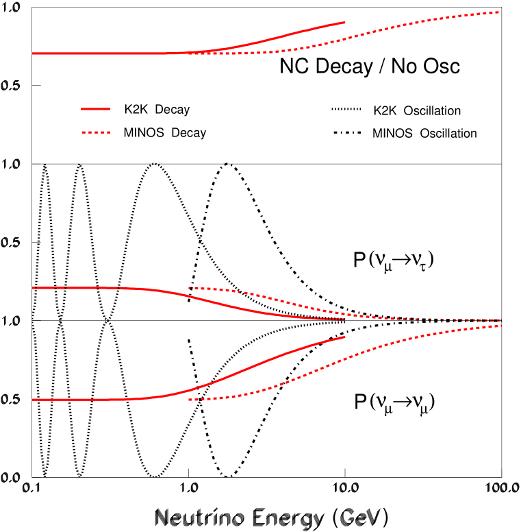
FIG. 3.: Long-baseline expectations for the K2K and MINOS long-baseline experiments from the decay model and the $\nu_{\mu}$–$\nu_{\tau}$ oscillation model. The upper panel gives the neutral current predictions compared to no oscillations (or $\nu_{\mu}$–$\nu_{\tau}$ oscillations).

REFERENCES

- [1] B. W. Lee, S. Pakvasa, R. Shrock and H. Sugawara, Phys. Rev. Lett. 38 (1977) 937; S. Treiman. F. Wilczek and A. Zee, Phys. Rev. D16 (1977) 152.
- [2] P. Langacker and D. London, Phys. Rev. D38 (1988) 907, S. Bergmann and A. Kagan, Nucl. Phys. B358 (1999) 368.
- [3] E. Roulet, Phys. Rev. D44 (1991) 935; M. M. Guzzo, A. Masiero and S. Petcov, Phys. Lett. B260 (1991) 154; V. Barger, R. J. N. Philips and K. Whisnant, Phys. Rev. D44 (1991) 1629.
- [4] L. Wolfenstein, Phys. Rev. D17 (1978) 2369.
- [5] M. Gasperini, Phys. Rev. D38 (1988) 2635; A. Halprin and C. N. Leung, Phys. Rev. Lett. 67 (1991) 1833.
- [6] S. Coleman and S. L. Glashow, Phys. Lett. B405 (1997) 249.
- [7] S. Glashow, A. Halprin, P. I. Krastev, C. N. Leung and J. Pantaleone, Phys. Rev. D56 (1977) 2433.
- [8] This discussion follows V. Barger, J. G. Learned, S. Pakvasa and T. J. Weiler, Phys. Rev. Lett. 82 (1999) 2640.
- [9] C. Athanassopoulos et al., the LSND Collaboration, Phys. Rev. Lett. 77 (1996) 3082; ibid 81 (1998) 1774.
- [10] Some discussion of these scenarios can be found in S. Bergmann and Y. Grossman, Phys. Rev. D59 (1999) 093005; L. M. Johnson and D. McKay, Phys. Lett. B433 (1998) 355 and P. Herczeg, Proceedings of International Conference on Particle Physics Beyond The Standard Model, Jun 8-14, 1997; Castle Ringberg, Germany; ed. by H. V. Klapdor-Kleingrothaus, (1998) 124.
- [11] Y. Grossman, (private communication).
- [12] J. N. Bahcall and P. Krastev, hep-ph/9703267; S. Bergmann, Nucl. Phys. B515 (1998) 363.
- [13] P. Krastev, (private communication).
- [14] S. W. Mansour and T-K. Kuo, hep-ph/9810510; see also A. Halprin, C. N. Leung and J. Pantaleone, Phys. Rev. D53 (1996) 5365; J. N. Bahcall, P. Krastev and C. N. Leung, Phys. Rev. D52 (1996) 1770; H. Minakata and H. Nunokawa, Phys. Rev. D51 (1995) 6625.
- [15] J. Pantaleone, T. K. Kuo and S.W. Mansour, hep-ph/9907478.
- [16] The CCFR Collaboration, A. Romosan, et al, Phys. Rev. D59 (1999) 031101, Phys. Rev. Lett. 78 (1997) 2912.
- [17] A.M. Gago, H. Nunokawa and R. Zukanovich-Funchal, hep-ph/9909250.
- [18] S. Pakvasa and K. Tennakone, Phys. Rev. Lett. 28 (1972) 1415; J. N. Bahcall, N. Cabibbo and A. Yahil, Phys. Rev. Lett. 28 (1972) 316; See also A. Acker, A. Joshipura and S. Pakvasa, Phys. Lett. B285 (1992) 371; Z. Berezhiani, G. Fiorentini, A. Rossi and M. Moretti, JETP Lett. 55 (1992) 151.
- [19] A. Acker and S. Pakvasa (in preparation); A. Acker and S. Pakvasa, Phys. Lett. B320 (1994) 320.
- [20] P. F. Harrison, D. H. Perkins and W. G. Scott, hep-ph/9904297; A. Acker, J. G. Learned, S. Pakvasa and T. J. Weiler, Phys. Lett. B298 (1993) 149; G. Conforto, M. Barone and C. Grimani, Phys. Lett. B447 (1999) 122; A. Strumia, JHEP 9904 (1999) 026.
- [21] M. C. Gonzales-Garcia, M. M. Guzzo, P. I. Krastev, H. Nunokawa, O. Peres, V. Pleitez, J. Valle and R. Zukanovich Funchal, Phys. Rev. Lett. 82 (1999) 3202; See also F. Brooijmans, hep-ph/9808498.
- [22] P. Lipari and M. Lusignoli, Phys. Rev. D60 (1999) 013003.
- [23] G. L. Fogli, E. Lisi and A. Marrone, hep-ph/9904248; G. L. Fogli, E. Lisi and A. Marrone, Phys. Rev. D59 (1999) 117303; S. Choubey and S. Goswami, hep/ph-9904257.
- [24] R. Foot, C. N. Leung and O. Yasuda, Phys. Lett. B443 (1998) 185.
- [25] Y. Fukuda et al.(the Super-Kamiokande Collaboration), Phys. Rev. Lett. 81 (1998) 1562; ibid, 82 (1998) 2644; T. Kajita hep-ex/9810001. The use of more recent data(K. Scholberg, hep-ex/9905016) does not change the conclusions.
- [26] V. Barger, J. G. Learned, P. Lipari, M. Lusignoli, S. Pakvasa and T. J. Weiler, hep-ph/9907421(Phys. Lett. B in press).
- [27] V. Barger, W-Y. Keung and S. Pakvasa, Phys. Rev. D25 (1982) 907.
- [28] J. Valle, Phys. Lett. 131B (1983) 87; G. Gelmini and J. Valle, ibid B142 (1983) 181; K. Choi and A. Santamaria, Phys. Lett. B267 (1991) 504; A. Joshipura and S. Rindani, Phys. Rev. D46 (1992) 300.
- [29] A. Joshipura (private communication).
- [30] T. Kajita, Super-Kamiokande results presented at the “Beyond the Desert” Workshop, Castle Ringberg, Tegernsee, Germany, June 6–12, 1999 (to be published in the proceedings).
- [31] V. Barger, N. Deshpande, P. Pal, R.J.N. Phillips and K. Whisnant, Phys. Rev. D43, 1759 (1991); E. Akhmedov, P. Lipari and M. Lusignoli, Phys. Lett. B300, 128 (1993).
- [32] J. Pantaleone, Phys. Rev. D49, 2152 (1994).
- [33] Q. Liu and A. Smirnov, Nucl. Phys. B524, 505 (1998); P. Lipari and M. Lusignoli, Phys. Rev. D58, 073005 (1998).
- [34] F. Vissani and A. Smirnov, Phys. Lett. B432, 376 (1998); J. Learned, S. Pakvasa, and J. Stone, Phys. Lett. B435, 131 (1998); L. Hall and H. Murayama, Phys. Lett. B436, 323 (1998).
- [35] KEK-PS E362, INS-924 report (1992).
- [36] MINOS Collaboration, NuMI-L-375 report (1998).
- [37] NGS report, CERN 98-02, INFN/AE-98/05 (1998).
- [38] R. Kolb and M. S. Turner, The Early Universe, Addison - Wesley (1990).
- [39] K. Olive and D. Thomas, hep-ph/9811444.
- [40] E. Lisi, S. Sarkar, F. Villante, Phys. Rev. D59, 123520 (1999).
- [41] S. Burles, K. Nollett, J. Truran and M. S. Turner, Phys. Rev. Lett. 82, 4176 (1999).
- [42] J. G. Learned and S. Pakvasa, Astropart. Phys. 3, (1995) 267; F. Halzen and D. Saltzberg, Phys. Rev. Lett. 81 (1998) 5722.
- [43] M. Apollonio et al. (the CHOOZ Collaboration), Phys. Lett. B420, 320 (1998).
- [44] For a review of accelerator limits, see K. Zuber, Phys. Rep. 305, 295 (1998).
- [45] Y. Grossman and M. Worah, hep-ph/9807511.