Abstract

We perform a combined analysis of the unitarity triangle and of the CP violating parameter $\varepsilon^{\prime}/\varepsilon$ using the most recent determination of the relevant experimental data and, whenever possible, hadronic matrix elements from lattice QCD. We discuss the rôle of the main non-perturbative parameters and make a comparison with other recent analyses. We use lattice results for the matrix element of $Q_{8}$ obtained without reference to the strange quark mass. Since a reliable lattice determination of the matrix element of $Q_{6}$ is still missing, the theoretical predictions for $\varepsilon^{\prime}/\varepsilon$ suffer from large uncertainties. By evaluating this matrix element with the vacuum-saturation approximation, we typically find as central value $\varepsilon^{\prime}/\varepsilon=(4\div 7)\times 10^{-4}$. We conclude that the experimental data suggest large deviation of the value of the matrix element of $Q_{6}$ from the vacuum-saturation approximation, possibly due to penguin contractions.

October 1999

1 Introduction

The latest measurements of $\varepsilon^{\prime}/\varepsilon$

$$\begin{array}[]{lll}\mbox{Re}(\varepsilon^{\prime}/\varepsilon)=(28.0\pm 4.1)\times 10^{-4}&\mbox{KTeV}&\cite[cite]{[\@@bibref{}{KTeVK99}{}{}]},\\ \mbox{Re}(\varepsilon^{\prime}/\varepsilon)=(18.5\pm 7.3)\times 10^{-4}&\mbox{NA48}&\cite[cite]{[\@@bibref{}{NA48K99}{}{}]},\end{array}$$ (1)

confirm the large value found by NA31 [3] and rise the world average to $\mbox{Re}(\varepsilon^{\prime}/\varepsilon)_{\mbox{(WA)}}=(21.2\pm 4.6)\times 10^{-4}$ [2]. Motivated by these results, we present a new study of the unitarity triangle and of CP violation in kaon decays within the Standard Model. Our results have been obtained from a Next-to-Leading Order (NLO) calculation of $\varepsilon^{\prime}/\varepsilon$ combined with the constraints on the Cabibbo-Kobayashi-Maskawa matrix ($V_{CKM}$) derived from measurements of $|V_{cb}|$, $|V_{ub}|$, $\varepsilon$, $\Delta M_{B_{d}}$ and the limits on $\Delta M_{B_{s}}$. This work is an upgraded and improved version of previous studies made by the Rome group [4]–[6]. Similar analyses can be found in the recent literature [7]–[15]. For previous estimates of $\varepsilon^{\prime}/\varepsilon$ with a heavy top mass see also [16]–[20].

Several features characterize this work:

• We analyze the constraints on $V_{CKM}$ together with $\varepsilon^{\prime}/\varepsilon$, fully taking into account correlation effects. This should be compared with the analyses of refs. [21, 22], where only the $V_{CKM}$ constraints were considered, or with the analyses of refs. [9, 10] and [14, 20], where the input values and errors of the $V_{CKM}$ parameters used in the study of $\varepsilon^{\prime}/\varepsilon$ were taken elsewhere. With respect to the recent study of ref. [13], we present the results of the analysis of the unitarity triangle together with the predictions for $\varepsilon^{\prime}/\varepsilon$.

• In our NLO analysis, we include the full, correlated dependence of the coefficients of the effective Hamiltonians ${\cal H}^{\Delta S=2}$, ${\cal H}^{\Delta B=2}$  and ${\cal H}^{\Delta S=1}$, computed in refs. [23]–[29], on the relevant parameters, such as $\alpha_{s}(M_{Z})$ or the $\overline{MS}$ top mass, $m_{t}^{\overline{MS}}(m_{t}^{\overline{MS}})$.

• We carefully account for the renormalization-scheme dependence of the matrix elements of the renormalized operators and of the compensating effects in the corresponding Wilson coefficients. This is specially important, given the large differences in the values of matrix elements of operators defined with different prescriptions, in particular for $Q_{6}$ and $Q_{8}$ .

• We address the issue of the dependence of theoretical predictions for $\varepsilon^{\prime}/\varepsilon$ on the strange quark mass $m_{s}$, induced by the standard definition of the $B$ parameters. In addition, we present results obtained by using the matrix elements of the electropenguin operators, $Q_{7}$ and $Q_{8}$, computed without any reference to the quark masses [30].

Our main results are the following. For the unitarity triangle, using experimental informations on $|V_{cb}|$, $|V_{ub}|$, $\varepsilon$, $\Delta M_{B_{d}}$ and $\Delta M_{B_{s}}$, we find

$$\begin{array}[]{l l}\overline{\rho}=0.16^{+0.08}_{-0.11}\,,&\overline{\eta}=0.38^{+0.06}_{-0.05}\,,\\ \sin(2\alpha)=0.11^{+0.40}_{-0.35}\,,&\sin(2\beta)=0.75^{+0.09}_{-0.09}\,,\\ \gamma=(68^{+15}_{-10})^{o}\,,&Im\lambda_{t}=(1.34^{+0.16}_{-0.15})\times 10^{-4}\,.\end{array}$$ (2)

in good agreement with the results of other recent studies [21, 22]. A detailed discussion of this analysis can be found in sect. 3.

Concerning $\varepsilon^{\prime}/\varepsilon$, the major uncertainty still affecting the theoretical predictions is the lack of a quantitative determination of the matrix element of $Q_{6}$. In particular, the status of lattice calculations for this matrix element is more confused now than a few years ago. The value obtained using staggered fermions, indicating small deviations from the vacuum-saturation approximation (VSA) for the bare operator [31], has been found plagued by huge perturbative corrections [32] which make it unreliable. Very recent results using domain-wall fermions [33], on the contrary, correspond to a dramatic violation of the VSA and predict a sign of the matrix element different from any other non-perturbative approach. Since this result has been obtained with a lattice formulation for which numerical studies began very recently, we think that further scrutiny and confirmation from other calculations are needed before using it in phenomenological analyses.

With this caveat in mind, we prefer to give firstly our result for $\varepsilon^{\prime}/\varepsilon$ in the form

$$\varepsilon^{\prime}/\varepsilon=\left[(-21.7^{+3.9}_{-4.3})\,\mbox{GeV}^{-3}\times\langle\pi\pi|Q_{6}^{HV}|K\rangle_{I=0}-(6.0^{+1.5}_{-1.8})\right]\times 10^{-4}\,,$$ (3)

where the operator $Q_{6}$ is renormalized at $\mu=2$ GeV in the ’t Hooft-Veltman ($HV$) renormalization scheme of ref. [27] and the errors are evaluated by varying all the experimental and theoretical parameters, but $\langle\pi\pi|Q_{6}^{HV}|K\rangle_{I=0}$, as explained in sect. 2. One may use this formula to estimate $\varepsilon^{\prime}/\varepsilon$ with any non-perturbative method able to control the renormalization scale and scheme dependence of $Q_{6}$ at the NLO.

In the absence of definite results from the lattice, we take the central value of $\langle\pi\pi|Q_{6}^{HV}|K\rangle_{I=0}$ from the VSA and allow a large variation of the matrix element using a relative error of $100\%$. Note that there is an ambiguity in taking this value, since the renormalization scheme and scale of the operator is unknown in the VSA. By assuming the VSA for the central value in the $HV$ scheme at $\mu=2$ GeV, we find

$$\begin{array}[]{l l}\varepsilon^{\prime}/\varepsilon=(3.6^{+6.7}_{-6.3}\pm 0.5)\times 10^{-4}&\mbox{(Monte Carlo),}\\ -11\times 10^{-4}\leq\varepsilon^{\prime}/\varepsilon\leq 27\times 10^{-4}&\mbox{(Scanning),}\end{array}$$ (4)

where the first error comes from the uncertainties on the input parameters and the second one accounts for the residual renormalization scheme dependence due to higher orders in the perturbative expansion. Details on the definition of the errors and the scanning procedure can be found in sect. 2. Taking the value of the VSA in the NDR scheme, we find instead

$$\begin{array}[]{l l}\varepsilon^{\prime}/\varepsilon=(6.7^{+9.2}_{-8.5}\pm 0.4)\times 10^{-4}&\mbox{(Monte Carlo),}\\ -10\times 10^{-4}\leq\varepsilon^{\prime}/\varepsilon\leq 30\times 10^{-4}&\mbox{(Scanning).}\end{array}$$ (5)

Note that the difference between eqs. (4) and (5) is not due to the scheme dependence, but to the change in the value of the matrix element of $Q_{6}$. For a more detailed discussion of this point, see sect. 4.

We conclude that, with a central value of $\langle\pi\pi|Q_{6}|K\rangle_{0}$ close to the VSA one, even with a large error, it is difficult to reproduce the experimental value of $\varepsilon^{\prime}/\varepsilon$, for which a conspiracy of several inputs pushing $\varepsilon^{\prime}/\varepsilon$ in the same direction is necessary. In our opinion, the important message arriving from the experimental results is that penguin contractions (eye diagrams), neglected in the VSA, give contributions to the matrix elements definitely larger than their factorized values. This interpretation provides a unique dynamical mechanism to account for both the $\Delta I=1/2$ rule and a large value of $\varepsilon^{\prime}/\varepsilon$ within the Standard Model, whereas other arguments, as those based on a low value of $m_{s}^{\overline{MS}}(\mu)$, would leave the $\Delta I=1/2$ rule unexplained.

This paper is organized as follows. In sect. 2, we describe the methods used in the phenomenological analysis. Our study of the unitarity triangle can be found in sect. 3. Details on the calculation of $\varepsilon^{\prime}/\varepsilon$ are given in sect. 4. In both cases, we make a comparison with other recent analyses. Section 5 contains our conclusions.

2 Analysis method

The analysis of the unitarity triangle is based on a comparison of theoretical expressions for $\varepsilon$, $\Delta M_{B_{d}}$ and $\Delta M_{B_{s}}$ with the measurements/bounds and on the experimental determination of $|V_{ub}|$ and $|V_{cb}|$. Several parameters enter the theoretical expressions of the above quantities. They can be classified in two groups: “experimental” quantities, such as the top and $W$ masses, $\alpha_{s}(M_{z})$, etc., and theoretical ones, such as the Wilson coefficients, which are computed at the NLO in perturbation theory, and the hadronic matrix elements.

We now describe the procedure used in our combined analysis of $\varepsilon^{\prime}/\varepsilon$ and the unitarity triangle.

1. For all the parameters which determine $\varepsilon$, $\Delta M_{B_{d}}$ and $\Delta M_{B_{s}}$, we extract randomly the experimental quantities with gaussian distributions and the theoretical ones with flat distributions . The latter include, for example, $\hat{B}_{K}$, the $b$-quark mass, which enters as a threshold in the evolution of the Wilson coefficients, etc. We have some remarks to make on the choice of the error distributions. In many cases, the main systematic error in the determination of the experimental quantities, such as $|V_{ub}|$, comes from the theoretical uncertainties. One may argue that systematic errors coming from the theory (and experimental-systematic errors as well) should correspond to flat distributions. In practice, it may be difficult to disentangle statistical and systematic errors affecting some input parameters. However, as discussed below, the actual choice of the error distributions has a rather small influence on the final results. For these reasons, we have assumed for all the experimental quantities gaussian distributions, with a width obtained by combining in quadrature all errors.

2. Among the quantities which are extracted with a gaussian distribution, there are also $|V_{ub}|$ and $|V_{cb}|$; for a given set of extracted values of $|V_{ub}|$, $|V_{cb}|$ and $\lambda=|V_{us}|$, we determine $\sigma=\sqrt{\rho^{2}+\eta^{2}}=|V_{ub}|/(\lambda|V_{cb}|)$.

3. For a given value of $\sigma$ (and of all the other relevant parameters), we extract a value of $\varepsilon$ with gaussian distribution, and find the solutions of the equation

   $$\varepsilon=\varepsilon^{th}(m_{t}^{\overline{MS}}(m_{t}^{\overline{MS}}),\alpha_{s}(M_{z}),\dots,\hat{B}_{K},\sigma,\delta)\,$$ (6)

   with respect to $\delta$, which is the CP violation phase in the standard parameterization of $V_{CKM}$ as adopted by the PDG [34], with $0\leq\delta\leq\pi$. In eq. (6), $\varepsilon^{th}(m_{t}^{\overline{MS}}(m_{t}^{\overline{MS}}),\alpha_{s}(M_{z}),\dots,\hat{B}_{K},\sigma,\delta)$ is the theoretical value computed for that given set of random parameters and $\varepsilon$ is the extracted value. The explicit expression of $\varepsilon^{th}$ can be found for example in eq. (10) of ref. [5]. In general one finds two independent solutions for $\delta$. For any set of extractions, this fixes two independent sets of values for $\rho=\sigma\cos\delta$ and $\eta=\sigma\sin\delta$. In the following, the set of all the extracted parameters and of one of the two solutions for $\rho$ and $\eta$ will be denoted as event . When we consider also $\varepsilon^{\prime}/\varepsilon$, event denotes all the random variables, including the matrix elements (and further parameters) which enter the calculation of this quantity.

4. For a given event, $n_{i}$, we compute a statistical weight defined as

   $${\cal W}_{i}=\exp\Bigg{[}-\frac{1}{2}\left(\frac{\Delta M_{B_{d}}^{exp}-\Delta M_{B_{d}}^{th}(n_{i})}{d\Delta M_{B_{d}}}\right)^{2}$$

   $$-\frac{1}{2}\left(\frac{a[\Delta M_{B_{s}}^{th}(n_{i})]-1}{da[\Delta M_{B_{s}}^{th}(n_{i})]}\right)^{2}\Bigg{]}\times J^{-1}\left[\left(|V_{ub}|,\varepsilon^{th}\right),\left(\rho,\eta\right)\right]\,,$$ (7)

   where $\Delta M_{B_{d}}^{th}(n_{i})$ and $\Delta M_{B_{s}}^{th}(n_{i})$ are the theoretical values of $\Delta M_{B_{d}}$ and $\Delta M_{B_{s}}$ computed with the event $n_{i}$; $a[\Delta M_{B_{s}}]$ and $da[\Delta M_{B_{s}}]$ are the average value and error of the oscillation amplitude for $B^{0}_{s}$–$\bar{B}^{0}_{s}$ mixing, introduced in ref. [35] . $J\left[\left(|V_{ub}|,\varepsilon^{th}\right),\left(\rho,\eta\right)\right]$ is the Jacobian relating $|V_{ub}|$ and $\varepsilon^{th}$ to $\rho$ and $\eta$. With this weight factor, our procedure coincides with the method followed in ref. [22]: in that case they extract with flat distributions $\rho$ and $\eta$, compute $|V_{ub}|(\rho,\eta)$ and $\varepsilon(\rho,\eta)$ and include in the statistical weight a factor

   $$\exp\left[-\frac{1}{2}\left(\frac{|V_{ub}^{exp}|-|V_{ub}|(\rho,\eta)}{d|V_{ub}|}\right)^{2}-\frac{1}{2}\left(\frac{\varepsilon^{exp}-\varepsilon(\rho,\eta)}{d\varepsilon}\right)^{2}\right]\,,$$ (8)

   instead of $J^{-1}$. Since the error on the measurement of $\varepsilon$ is tiny, most of the extractions of $\rho$ and $\eta$ in the interval $[0,1]$, correspond to very small statistical weights. Thus, the method of ref. [22] demands a large number of extractions in order to obtain a significative statistical sample. Our procedure is, in this respect, more efficient.

   Constant	Values
   $G_{F}$	$1.16639\times 10^{-5}\,\mbox{GeV}^{-2}$
   $\alpha_{e}(M_{z})$	$7.8125\times 10^{-3}$
   $\sin^{2}\theta_{w}$	0.23154
   $f_{\pi}$	0.1307 GeV
   $f_{K}$	0.1598 GeV
   $M_{W}$	80.41 GeV
   $M_{Z}$	91.1867 GeV
   $M_{B_{d}}$	5.2792 GeV
   $M_{B_{s}}$	5.3693 GeV
   $M_{K^{0}}$	0.498 GeV
   $M_{\pi}$	0.140 GeV
   $\Delta M_{K}$	$5.301\times 10^{9}\,\mbox{sec}^{-1}$
   $\omega$	0.045
   $\mbox{Re}A_{0}$	$2.7\times 10^{-7}$ GeV
   $B_{7-9}^{1/2}$	1
   $\mu$	$2$ GeV

   Table 1: Constants used in the numerical analysis.

5. The statistical weight ${\cal W}_{i}$, suitably normalized to the sum over all the events, is used to compute averages and errors of the different quantities of interest. Since the probability distributions are in general non-gaussian, we give the “median” and the $68\%$ confidence level intervals. The median is defined in such a way that half of the weighted events lies below its value. The error range contains $68\%$ of the total weighted events. Occasionally we will also give standard averages and errors, or ranges obtained by scanning the relevant parameters. A meaningful definition of the scanning procedure requires the “gaussian” variables to be extracted uniformly within some range. We choose a range $\pm 1\sigma$ around the central values.

We have divided the input parameters into two groups:

• in table 1, quantities for which the error is so small to give negligible effects in our analysis are listed. In this table, we also give the value of the renormalization scale $\mu$ at which Wilson coefficients and operator matrix elements are evaluated (this has not been varied) and the values which have been taken for $B_{7-9}^{1/2}$. These matrix elements have never been computed on the lattice and our choice is just a guess, biased by the VSA and justified by the fact that the precise value of these $B$ parameters is not very important to the estimate of $\varepsilon^{\prime}/\varepsilon$, see fig. 3.

• in table 2, quantities which are extracted with gaussian (above the double horizontal line) or flat (below the double line) distributions are listed. The value of $|V_{ub}|$ is our average, and estimate of the error, of the CLEO [36] and LEP [37] measurements. The lattice results comes from our compilation of several lattice calculations. In the table, only $B$ parameters of left-left operators in the $HV$-scheme are listed. For these operators, the physical matrix elements can be readily obtained by multiplying physical quantities (such as $f_{K}$ or $M_{K^{0}}$) times the $B$ parameters, since the quark masses never enter their VSA expressions.

Parameter	Value and error
$V_{cb}$	$0.0395\pm 0.0017$
$V_{ub}$	$0.0037\pm 0.0007$
$\lambda$	$0.2196\pm 0.0023$
$\alpha_{s}(M_{z})$	$0.119\pm 0.003$
$\varepsilon$	$(2.28\pm 0.019)\times 10^{-3}$
$\Delta M_{B_{d}}$	$(0.472\pm 0.016)\times 10^{12}\,\mbox{sec}^{-1}$
$m_{t}^{\overline{MS}}(m_{t}^{\overline{MS}})$	$165\pm 5$ GeV
$m_{b}^{\overline{MS}}(m_{b}^{\overline{MS}})$	$4.25\pm 0.15$ GeV
$m_{c}^{\overline{MS}}(m_{c}^{\overline{MS}})$	$1.3\pm 0.2$ GeV
$f_{B_{d}}\sqrt{\hat{B}_{B_{d}}}$	$210\pm 30$ MeV
$f^{2}_{B_{d}}\hat{B}_{B_{d}}/f^{2}_{B_{s}}\hat{B}_{B_{s}}$	$1.14\pm 0.06$
$\Omega_{IB}$	$0.25\pm 0.15$
$\hat{B}_{K}$	$0.87\pm 0.13$
$B$ parameters in the $HV$-scheme at $\mu=2$ GeV
$B_{1}^{c}$	$0.075\pm 0.075$
$B_{2}^{c}$	$0.075\pm 0.075$
$B_{3}$	$3.5\pm 2.5$
$B_{4}$	$3.5\pm 2.5$
$B_{5,6}$	see eqs. (17) and (18)
$B_{7,8}^{3/2}$	see eq. (15)
$B_{9}^{3/2}$	$0.63\pm 0.09$

Table 2: Variable parameters: average and errors, $\bar{x}\pm dx$. The quantities above and below the double horizontal line have been extracted with gaussian and flat probability distributions, respectively. Matrix elements of left-left operators are expressed in terms of $B$ parameters and measurable quantities (such $f_{K}$, $M_{K^{0}}$, etc.) only. In these cases, it is equivalent to quote the value of the matrix elements or the $B$ parameters. The latter are listed in this table.

Central values and errors of all the results presented in this study correspond to the “median” and the $68\%$ confidence-level region of the appropriate distributions. In some cases, we also give ranges obtained by scanning all the input parameters.

3 Constraints on the Unitarity Triangle

Analyses of the unitarity triangle and NLO calculations of $\varepsilon^{\prime}/\varepsilon$ have been around for several years [4]–[8],[19, 21, 22, 38]. As discussed in the previous section, this analysis is based on a comparison of theoretical expressions for $\varepsilon$, $\Delta M_{B_{d}}$ and $\Delta M_{B_{s}}$ with the measurements/bounds and on the experimental determinations of $|V_{ub}|$ and $|V_{cb}|$. All relevant theoretical formulae can be found in refs. [4]–[8], [13, 19]. Expressions, and numerical values, of the Wilson coefficients appearing in the effective Hamiltonians, in all popular renormalization schemes, can also be found in refs. [5, 7, 8],[25]–[27]. The values of the input parameters can be found in tables 1 and 2.

The results of our analysis of the unitarity triangle are given in eq. (2). These values correspond to the density plot in the $\bar{\rho}$–$\bar{\eta}$ plane shown in fig. 1.

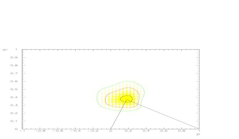
Figure 1: Density plot in the $\bar{\rho}$–$\bar{\eta}$ plane. Contours define regions containing $5\%$, $68\%$ and $95\%$ of the generated events

Since the fit to the unitarity triangle is overconstrained, one can extract one (or more) input variables, such as the renormalization group invariant $\hat{B}_{K}$ or $f_{B_{d}}\sqrt{\hat{B}_{B_{d}}}$, together with the CKM parameters [21, 22]. By removing the bounds on one of the above theoretical quantities, we obtain respectively

$$\hat{B}_{K}=0.90^{+0.26}_{-0.16}\,,\quad f_{B_{d}}\sqrt{\hat{B}_{B_{d}}}=224^{+23}_{-25}\;\mbox{MeV}\,.$$ (9)

These results are in very good agreement with predictions from lattice QCD, for example $\hat{B}_{K}=0.89\pm 0.14$ [39] (our average from a compilation of lattice results for $\hat{B}_{K}$ is given in table 2) and $f_{B_{d}}\sqrt{\hat{B}_{B_{d}}}=210\pm 20\pm 20$ MeV [40] (for a recent review, see also ref. [41]). It is worth noting that lattice predictions for these quantities existed long before the possibility of extracting them from the analysis of the unitarity triangle and have been very stable over the years .

Comparison with other analyses

We now briefly compare our results with the two recent analyses of refs. [21] and [22].

In spite of several differences in the procedure followed in the analysis of the data, our results in eq. (2) are in very good agreement with those of ref. [21], which quotes 

$$\begin{array}[]{lll}\overline{\rho}=0.156^{+0.092}_{-0.068}\,,&\overline{\eta}=0.372^{+0.060}_{-0.057}\,,&\\ \sin(2\alpha)=0.06^{+0.35}_{-0.42}\,,&\sin(2\beta)=0.75\pm 0.090\,,&\gamma=(67^{+11}_{-12})^{o}\,.\end{array}$$ (10)

Although our method is equivalent to that of ref. [22], there are differences between their results,

$$\begin{array}[]{lll}\overline{\rho}=0.202^{+0.053}_{-0.059}\,,&\overline{\eta}=0.340\pm 0.035\,,&\\ \sin(2\alpha)=-0.26^{+0.29}_{-0.28}\,,&\sin(2\beta)=0.725^{+0.050}_{-0.060}\,,&\gamma=(59.5^{+8.5}_{-7.5})^{o}\,,\end{array}$$ (11)

and those in eq. (2). The main reason is the range chosen for $f_{B_{d}}\sqrt{\hat{B}_{B_{d}}}$ (and to some extent for $|V_{cb}|$) : in ref. [22] the central value is similar to ours, and to the value used by ref. [21], but the error is strongly asymmetric favouring larger values of $f_{B_{d}}\sqrt{\hat{B}_{B_{d}}}$. This choice is justified by arguing that the existing unquenched results for $f_{B_{d}}$ are larger than the corresponding quenched ones. This is not a good argument, however, because the effect of quenching on the $B$ parameter, i.e. on the full matrix element parametrized by $f_{B_{d}}\sqrt{\hat{B}_{B_{d}}}$, is still unknown and could compensate the increase of $f_{B_{d}}$. Thus, for this quantity, we have chosen the symmetric range in table 2. Given the strong correlation between $\bar{\rho}$ and $f_{B_{d}}\sqrt{\hat{B}_{B_{d}}}$, as shown in fig. 2, this choice accounts for the bulk of the differences in the results. We checked that, with a similar range for $f_{B_{d}}\sqrt{\hat{B}_{B_{d}}}$, our results are much closer to those of ref. [22].

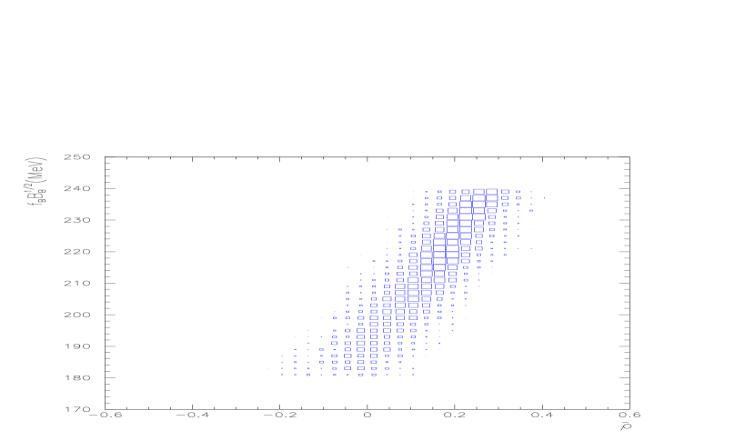
Figure 2: Density plot showing the correlation between $\bar{\rho}$ and $f_{B_{d}}\sqrt{\hat{B}_{B_{d}}}$.

Besides other minor differences in the range of the input parameters, the various analyses also differ in the treatment of the errors. The authors of ref. [22] attempt to distinguish, for each input parameter, statistical and systematic errors and assign to them different distributions. In ref. [21], all the relevant input variables are included in the expression of the $\chi^{2}$-function to be minimized, implicitly assuming gaussian distributions for all these quantities. In our case, we have defined two classes of statistical- and systematic-dominated parameters (see table 2), and use a single distribution, either gaussian or flat, for each variable. Finally, both refs. [21] and [22] consider the Wilson coefficients relevant to $K$ and $B$ meson mixing as independent input parameters, assuming for them either gaussian or flat distributions. This is not appropriate since the QCD corrections are known functions of $\alpha_{s}$, $m_{t}$, etc. and not independent quantities. In our analysis, for each event, we have computed the NLO QCD corrections, thus taking correctly into account the correlations.

Apart from the choice of the range of $f_{B_{d}}\sqrt{\hat{B}_{B_{d}}}$, these further differences have small effect on the final results for the unitarity triangle. In addition, the fitted values of $\hat{B}_{K}$ and $f_{B_{d}}\sqrt{\hat{B}_{B_{d}}}$ in eq. (9) are well consistent with the results of ref. [22], where they found $\hat{B}_{K}=0.87^{+0.34}_{-0.20}$ and $f_{B_{d}}\sqrt{\hat{B}_{B_{d}}}=223\pm 13$ MeV (Scenario I), and with those of ref. [21], $\hat{B}_{K}=0.80^{+0.27}_{-0.16}$ and $f_{B_{d}}\sqrt{\hat{B}_{B_{d}}}=222^{+26}_{-11}$ MeV.

4 Calculation of $\varepsilon^{\prime}/\varepsilon$

In this section, we summarize the main steps necessary to the calculation of $\varepsilon^{\prime}/\varepsilon$ and give some details on the procedure followed to obtain the result quoted in eq. (3)–(5). We also make a critical comparison with previous calculations of the Rome group [4]–[6], with the recent estimates of ref. [13] and with results obtained in other approaches such as the $\chi$QM [9, 10] and the $1/N$ expansion [14, 20].

Some general remarks are necessary before entering a more detailed discussion. Given the large numerical cancellations which may occur in the theoretical expression of $\varepsilon^{\prime}/\varepsilon$, a solid prediction should avoid the “Harlequin procedure”. This procedure consists in patching together $B_{6}$ from the $\chi$QM, $B_{8}$ from the $1/N$ expansion, $m_{s}^{\overline{MS}}(\mu)$ from the lattice, etc., or any other combination/average of different methods. All these quantities are indeed strongly correlated (for example $B_{6}$ and $B_{8}$ in the $1/N$ expansion or $B$ parameters and quark masses in the lattice approach) and should be consistently computed within each given theoretical framework. Unfortunately, as will clearly appear from the discussion below, no one of the actual non-perturbative methods is in the position to avoid completely the Harlequin procedure, not even for the most important input parameters only. The second important issue is the consistency of the renormalization procedure adopted in the perturbative calculation of the Wilson coefficients and in the non-perturbative computation of the operator matrix elements. This problem is particularly serious for the $\chi$QM and the $1/N$ expansion, and will be discussed when comparing the lattice approach to these methods. We will address, in particular, the problem of the quadratic divergences appearing in the $1/N$ expansion. This is an important issue, since the authors of refs. [14, 44] find that these divergences provide the enhancement necessary to explain the large values of Re$A_{0}$ and of $\varepsilon^{\prime}/\varepsilon$.

Schematically, $\varepsilon^{\prime}$ can be cast in the form

$$\varepsilon^{\prime}=\frac{\exp(i\pi/4)}{\sqrt{2}}\frac{\omega}{\mbox{Re}A_{0}}\times\left[\omega^{-1}\mbox{Im}A_{2}-(1-\Omega_{IB})\mbox{Im}A_{0}\right]$$ (12)

where $\omega=\mbox{Re}A_{2}/\mbox{Re}A_{0}$ and $\mbox{Re}A_{0}$, given in table 1, are taken from experiments, and $\Omega_{IB}$ is a correcting factor, estimated in refs. [45]–[47], due to isospin-breaking effects. Using the operator product expansion, the $K\to\pi\pi$ amplitudes Im$A_{2}$ and Im$A_{0}$ are computed from the matrix elements of the effective Hamiltonian, expressed in terms of Wilson coefficients and renormalized operators

$$\langle\pi\pi|{\cal H}^{\Delta S=1}|K^{0}\rangle=-\frac{G_{F}}{\sqrt{2}}\sum_{i}C_{i}(\mu)\langle\pi\pi|Q_{i}(\mu)|K^{0}\rangle\,$$ (13)

where the sum is over a complete set of operators, which depend on the renormalization scale $\mu$. In general, there are ten four-fermion operators and two dimension-five operators representing the chromo- and electro-magnetic dipole interactions. In the Standard Model, the contribution of these dimension-five operators is usually neglected (possible SUSY effects can enhance the contribution of the chromomagnetic operator [48]) and, with the scale $\mu=2$ GeV $>m_{c}$ at which calculations are performed  only 9 out of the 10 four-fermion operators are independent [26, 27]. Wilson coefficients and matrix elements of the operators $Q_{i}(\mu)$, appearing in the effective Hamiltonian, separately depend on the choice of the renormalization scale and scheme. This dependence cancels in physical quantities, such as Im$A_{2}$ and Im$A_{0}$, up to higher-order corrections in the perturbative expansion of the Wilson coefficients. For this crucial cancellation to take place, the non-perturbative method used to compute hadronic matrix elements must allow a definition of the renormalized operators consistent with the scheme used in the calculation of the Wilson coefficients.

So far, lattice QCD is the only non-perturbative approach in which both the scale and scheme dependence can be consistently accounted for, using either lattice perturbation theory or non-perturbative renormalization techniques [49, 50]. This is the main reason why we have followed this approach over the years.

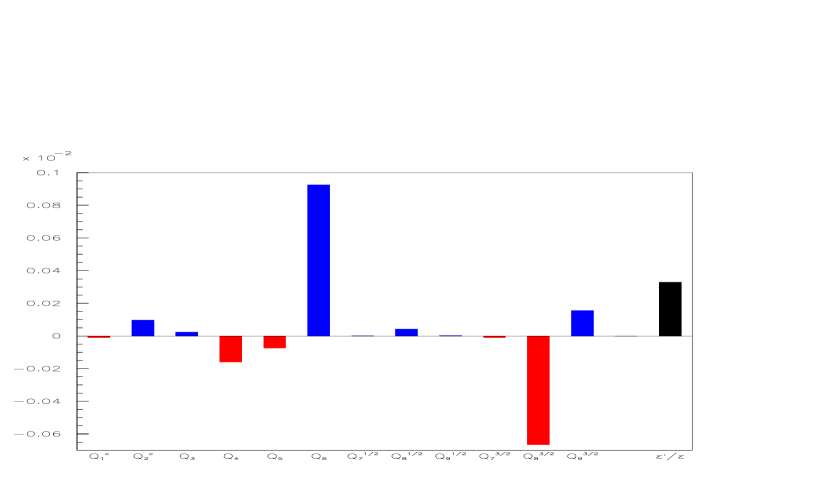
Figure 3: Individual contribution of the different operators to $\varepsilon^{\prime}/\varepsilon$, using the value of $\langle Q_{6}\rangle_{0}$ in eq. (17). The corresponding value of $\varepsilon^{\prime}/\varepsilon$ is also shown.

In fig. 3, we display the individual contributions of each operator to the prediction of $\varepsilon^{\prime}/\varepsilon$ using matrix elements computed on the lattice, as explained in the next section. Qualitatively, very similar results are obtained also in other approaches [10, 13, 14]. There is a general consensus that the largest contributions to $\varepsilon^{\prime}/\varepsilon$ are those coming from $Q_{6}$ and $Q_{8}$, with opposite sign, and sizeable contributions may come from $Q_{4}$, $Q_{5}$ and $Q_{9}$ in the presence of large cancellations between $Q_{6}$ and $Q_{8}$, i.e. when the prediction for $\varepsilon^{\prime}/\varepsilon$ is of ${\cal O}(10^{-4})$ . For this reason the following discussion, and the comparison with other calculations, will be focused on the determination, and errors, of the matrix elements of the two most important operators. In the following, we adopt the following notation:

$$\langle Q_{j}\rangle_{\{0,2\}}\equiv\langle\pi\pi|Q^{HV}_{j}(\mu=2\mbox{ GeV})|K^{0}\rangle_{I=\{0,2\}}$$ (14)

where the superscript denotes the $HV$ renormalization scheme as defined in ref. [27] .

Status of the calculation with matrix elements from lattice QCD

The evaluation of physical $K\to\pi\pi$ matrix elements on the lattice relies on the use of Chiral Perturbation Theory ($\chi$PT): so far only $\langle\pi|Q_{i}(\mu)|K\rangle$ and $\langle\pi(\vec{p}=0)\pi(\vec{q}=0)|Q_{i}(\mu)|K\rangle_{I=2}$ (with the two pions at rest) have been computed for a variety of operators. The physical matrix elements are then obtained by using $\chi$PT at the lowest order. This is a consequence of the difficulties in extracting physical multiparticle amplitudes in Euclidean space-time [51]. Proposals to overcome this problem have been presented, at the price of introducing some model dependence in the lattice results [52]. The use of $\chi$PT implies that large systematic errors may occur in the presence of large corrections from higher-order terms in the chiral expansion and/or from final-state interactions (FSI). This problem is common to all approaches: if large higher-order terms in the chiral expansion are indeed present and important, any method claiming to have these systematic errors under control must be able to reproduce the FSI phases $\delta_{0}$ and $\delta_{2}$ of the physical amplitudes. The approaches of ref. [9, 10] and [14], however, give FSI smaller than their physical values. Regarding this issue, we note that the idea of improving the predictions of the hadronic amplitudes using the experimental values of the FSI phases, with formulae such as $\langle Q_{i}\rangle_{I}\to Re\langle Q_{i}\rangle_{I}/\cos\delta^{exp}_{I}$, is illusory. If the FSI phases are not theoretically under control, one cannot tell whether the main uncertainty comes from the real or the imaginary part of the computed amplitude, or from the absolute value needed to compute $A_{0}$ and $A_{2}$.

$I=2$ matrix element of $Q_{8}$. There exists a large set of quenched calculations of $\langle Q_{8}\rangle_{2}$ performed with different formulations of the lattice fermion actions (Staggered, Wilson, tree-level improved, tadpole improved) and renormalization techniques (perturbative, boosted perturbative, non-perturbative), at several values of the inverse lattice spacing $a^{-1}=2\div 3$ GeV [30, 50],[53]–[55]. All these calculations, usually expressed in terms of $B_{8}^{(3/2)}$, give consistent results within $20\%$ of uncertainty. Among the results, we have taken the central value from the recent calculation of ref. [30], where the matrix elements $\langle Q_{8}\rangle_{2}$ and $\langle Q_{7}\rangle_{2}$ have been computed directly without any reference to the quark masses, and inflated the errors to account from the uncertainty due to the quenched approximation (unquenched results are expected very soon) and the lack of extrapolation to zero lattice spacing. The values we use are

$$\langle Q_{7}\rangle_{2}=0.18\pm 0.06\,{\rm GeV}^{3}\,,$$

$$\langle Q_{8}\rangle_{2}=0.62\pm 0.12\,{\rm GeV}^{3}\,.$$ (15)

The operator matrix elements computed without reference to quark masses are given in physical units. The reader who likes to work with $B$ parameters and quark masses may use the formulae

$$\langle Q_{7}(\mu)\rangle_{2} = \sqrt{2}f_{\pi}\left[\frac{1}{3}\left(\frac{M_{K^{0}}^{2}}{m_{s}^{\overline{MS}}(\mu)+m_{d}^{\overline{MS}}(\mu)}\right)^{2}-\frac{M_{K^{0}}^{2}-M_{\pi}^{2}}{2}\right]B^{(3/2)}_{7}(\mu)\,,$$

$$\langle Q_{8}(\mu)\rangle_{2} = \sqrt{2}f_{\pi}\left[\left(\frac{M_{K^{0}}^{2}}{m_{s}^{\overline{MS}}(\mu)+m_{d}^{\overline{MS}}(\mu)}\right)^{2}-\frac{M_{K^{0}}^{2}-M_{\pi}^{2}}{6}\right]B^{(3/2)}_{8}(\mu)\,.$$ (16)

The values of the matrix elements in eq. (15) correspond to $B_{7}^{(3/2)}=0.89\pm 0.30$ and $B^{(3/2)}_{8}=0.93\pm 0.18$ for a “conventional” mass fixed to $m_{s}^{\overline{MS}}+m_{d}^{\overline{MS}}=130$ MeV at $\mu=2$ GeV. Anybody may rescale the value of the $B$ parameters for these operators according to her/his preferred value for $m_{s}^{\overline{MS}}(\mu)$.

Matrix element of $Q_{6}$. For $\langle Q_{6}\rangle_{0}$ from the lattice, the situation appears worse today than a few years ago when the calculations of refs. [4]–[6] were performed:

• until 1997, the only existing lattice result, obtained with staggered fermions (SF) without NLO lattice perturbative corrections, was $B_{6}=1.0\pm 0.2$ [31]. This is the value used in our previous analyses [4, 5];

• with SF even more accurate results have been quoted recently, namely $B_{6}=0.67\pm 0.04\pm 0.05$ (quenched) and $B_{6}=0.76\pm 0.03\pm 0.05$ (with $n_{f}=2$) [56];

• ${\cal O}(\alpha_{s})$ corrections, necessary to match lattice operators to continuum ones at the NLO, are so huge for $Q_{6}$ with SF (in the neighborhood of $-100\%$ [32]) as to make all the above results unreliable. Note, however, that the corrections tend to diminish the value of $\langle Q_{6}\rangle_{0}$;

• the latest lattice results for this matrix element, computed with domain-wall fermions from $\langle\pi|Q_{6}|K\rangle$ [33], are absolutely surprising: $\langle Q_{6}\rangle_{0}$ has the sign opposite to what expected in the VSA, and to what is found with the $\chi$QM and the $1/N$ expansion. Moreover, the absolute value is so large as to give $\varepsilon^{\prime}/\varepsilon\sim-120\times 10^{-4}$. Were this confirmed, even the conservative statement by Andrzej Buras [57], namely … that certain features present in the Standard Model are confirmed by the experimental results. Indeed the sign and the order of magnitude of $\varepsilon^{\prime}/\varepsilon$ predicted by the Standard Model turn out to agree with the data… would result too optimistic. In order to reproduce the experimental number, $\varepsilon^{\prime}/\varepsilon\sim 20\times 10^{-4}$, not only new physics is required, but a large cancellation should also occur between the Standard Model and the new physics contributions. Since this result has been obtained with domain-wall fermions, a lattice formulation for which numerical studies began very recently, and no details on the renormalization and subtraction procedure have been given, we consider it premature to use the value of the matrix element of ref. [33] in phenomenological analyses. Hopefully, new lattice calculations will clarify this fundamental issue.

• estimates in the framework of the $1/N$ expansion (where, however, one should always to take into account the correlation between the values of $B_{6}$ and $B^{(3/2)}_{8}$ [58]) and by the $\chi$QM [10] give $B_{6}=0.7\div 1.3$ at scale $\mu=0.6\div 1.0$ GeV. One may argue [13, 58] that the scale dependence of $B_{6}$ above 1 GeV is rather weak and take the range $B_{6}=0.7\div 1.3$ as valid also at $\mu=2$ GeV, which is the scale at which we work. Note, however, that the dependence of the matrix elements on the renormalization scheme is rather strong and that, in these approaches, the scheme in which matrix elements are computed is unknown.

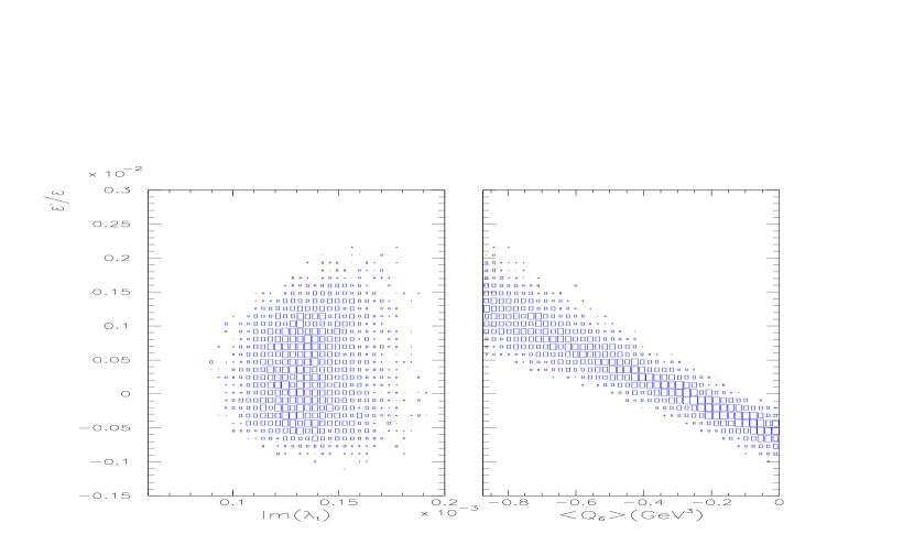
Figure 4: Density plots showing the correlation of Im $\lambda_{t}$ and $\langle Q_{6}\rangle_{0}$ with $\varepsilon^{\prime}/\varepsilon$.

Taking into account i)–v), we conclude that there is no computation of $\langle Q_{6}\rangle$ that can be reliably used in phenomenological analyses. For this reason, we present our result as in eq. (3). In addition, biased by the VSA, we give results assuming $B_{6}^{HV}=1.0\pm 1.0$ and $B_{6}^{HV}=1.35\pm 1.35$ (which corresponds to $B_{6}^{NDR}=1.0\pm 1.0$), taking an error of $100\%$. We compute the corresponding matrix element with the same “conventional” quark mass used for $\langle Q_{8}\rangle_{2}$, for which an explicit lattice calculation without reference to the quark masses exists. In physical units, this choice corresponds to

$$\langle Q_{6}\rangle_{0}=-0.4\pm 0.4\,{\rm GeV}^{3}\,,$$ (17)

and

$$\langle Q_{6}\rangle_{0}=-0.6\pm 0.6\,{\rm GeV}^{3}\,,$$ (18)

and $\langle Q_{5}\rangle_{0}=1/3\langle Q_{6}\rangle_{0}$, in the two cases. These expressions are obtained using the formulae

$$\langle Q_{5}(\mu)\rangle_{0} = -\frac{4}{3}\left(\frac{M_{K^{0}}^{2}}{m_{s}^{\overline{MS}}(\mu)+m_{d}^{\overline{MS}}(\mu)}\right)^{2}(f_{K}-f_{\pi})B_{5}(\mu)\,,$$

$$\langle Q_{6}(\mu)\rangle_{0} = -4\left(\frac{M_{K^{0}}^{2}}{m_{s}^{\overline{MS}}(\mu)+m_{d}^{\overline{MS}}(\mu)}\right)^{2}(f_{K}-f_{\pi})B_{6}(\mu)\,.$$ (19)

The values of $\varepsilon^{\prime}/\varepsilon$ obtained using the matrix elements in eqs. (17) and (18) are given in eqs. (4) and (5) respectively. The large difference between the two results is due to the strong correlation between $\varepsilon^{\prime}/\varepsilon$ and $\langle Q_{6}\rangle$, as shown in fig. 4. In the same figure we also show the correlation between $\varepsilon^{\prime}/\varepsilon$ and $Im\lambda_{t}$, which is the parameter governing the strength of CP violation in $K$-meson decays.

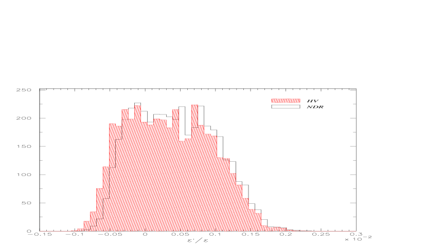
Figure 5: Probability distribution of $\varepsilon^{\prime}/\varepsilon$ in the $HV$ and $NDR$ schemes. In changing schemes matrix elements and Wilson coefficients have been consistently redefined at the NLO.

In fig. 5, we give two event distributions of $\varepsilon^{\prime}/\varepsilon$, obtained using Wilson coefficients and hadronic matrix elements consistently computed in $HV$ and $NDR$. Indeed, the calculation of the Wilson coefficients achieved in refs. [5, 7, 8], [23]–[27] allows a consistent determination of the matrix elements of the renormalized operators at the NLO. Notice that the two distributions in fig. 5 are quite similar, while differences between matrix elements in different schemes can be rather large: the parameter $B_{6}$ decreases, for instance, by $\sim 30\%$ going from the $HV$ to the $NDR$ scheme. This decrease is, however, largely compensated by a readjustment of the corresponding Wilson coefficients, as must happen in NLO calculations. The uncertainties due to higher order perturbative corrections, given by the second error in eqs. (4) and (5), have been evaluated by modifying consistently Wilson coefficients and matrix elements in the $HV$ and $NDR$ schemes. In the two cases, using for example $\langle Q_{6}\rangle_{0}$ from eq. (17), we obtain

$$\varepsilon^{\prime}/\varepsilon = (3.1^{+6.7}_{-6.3})\times 10^{-4}\quad HV\,,$$

$$\varepsilon^{\prime}/\varepsilon = (4.0^{+6.5}_{-6.1})\times 10^{-4}\quad NDR\,,$$ (20)

from which the result in eq. (4) has been derived.

The results in eqs. (4) and (5) are in very good agreement with previous estimates of the Rome [4]–[6] and Munich group [7, 8]. This agreement it is not surprising since the two groups are using very similar inputs for the matrix elements and the experimental parameters have only slightly changed in the last few years. The crucial problem, namely a quantitative determination of $\langle Q_{6}\rangle_{0}$, remains unfortunately still unsolved. At present, we can only conclude that, with the central value of $\langle Q_{6}\rangle_{0}$ taken from the VSA, even with a large error, it is difficult to reproduce the experimental value of $\varepsilon^{\prime}/\varepsilon$. On the other hand, by scanning various input parameters ($\alpha_{s}(M_{Z})$, $Im\lambda_{t}$, etc. and, in the conventional approach, $B_{6}$ and $B_{8}^{(3/2)}$) and in particular by choosing them close to their extreme values, it is possible to obtain $\varepsilon^{\prime}/\varepsilon$ up to $30\times 10^{-4}$. This gives the impression of a better agreement (lesser disagreement) between the theoretical predictions and the data. For completeness, we also give the interval of values of $\varepsilon^{\prime}/\varepsilon$ obtained by scanning, within one $\sigma$ the different parameters. We obtain

$$-11\times 10^{-4}\leq \varepsilon^{\prime}/\varepsilon \leq 27\times 10^{-4}\,,$$

$$-10\times 10^{-4}\leq \varepsilon^{\prime}/\varepsilon \leq 30\times 10^{-4}\,,$$ (21)

using $\langle Q_{6}\rangle_{0}$ from eqs. (17) and (18) respectively. Equation (21) allows a direct comparison with several calculations appeared in the literature

$$\begin{array}[]{ll}0.2\times 10^{-4}\leq\varepsilon^{\prime}/\varepsilon\leq 22.0\times 10^{-4}&\mbox{Munich99-HV~{}\cite[cite]{[\@@bibref{}{silvestrini}{}{}]}},\\ 1.1\times 10^{-4}\leq\varepsilon^{\prime}/\varepsilon\leq 28.8\times 10^{-4}&\mbox{Munich99-NDR},\\ 7.0\times 10^{-4}\leq\varepsilon^{\prime}/\varepsilon\leq 31\times 10^{-4}&\mbox{Trieste98~{}\cite[cite]{[\@@bibref{}{bert2}{}{}]}},\\ 1.5\times 10^{-4}\leq\varepsilon^{\prime}/\varepsilon\leq 31.6\times 10^{-4}&\mbox{Dortmund99~{}\cite[cite]{[\@@bibref{}{paschoslast}{}{}]}}.\end{array}$$ (22)

Note that our scanning results include a region of negative $\varepsilon^{\prime}/\varepsilon$ on account of our choice of the error on $\langle Q_{6}\rangle_{0}$ being larger than in other cases.

In spite of the fact that the experimental world average is compatible with the above “scanned” ranges, we stress that, in order to get a large value of $\varepsilon^{\prime}/\varepsilon$, a conspiracy of several inputs pushing $\varepsilon^{\prime}/\varepsilon$ in the same direction is necessary. For central values of the parameters, the predictions are, in general, much lower than the experimental results. For example, the Rome-Munich and $1/N$ estimates are typically in the range $3$–$8\times 10^{-4}$ and $8$–$10\times 10^{-4}$, respectively. For this reason, barring the possibility of new physics effects [48], we believe that an important message is arriving from the experimental results:

penguin contractions (or eye diagrams, not to be confused with penguin operators [60]), usually neglected within factorization, give contributions to the matrix elements definitely larger than their factorized values.

This implies that the “effective” $B$ parameters of the relevant operators, specifically those relative to the matrix elements of $Q_{1}$ and $Q_{2}$ for Re$A_{0}$ and of $Q_{6}$ for $\varepsilon^{\prime}/\varepsilon$ are much larger than one. This interpretation would provide a unique dynamical mechanism to explain both the $\Delta I=1/2$ rule and a large value of $\varepsilon^{\prime}/\varepsilon$ [61]. Large contributions from penguin contractions are actually found by calculations performed in the framework of the Chiral Quark Model ($\chi$QM) [9, 10] or the $1/N$ expansion [14, 20, 62]–[44]. It is very important that these indications find quantitative confirmation in other approaches, for example in lattice QCD calculations. Note that naïve explanations of the large value of $\varepsilon^{\prime}/\varepsilon$, such as a very low value of $m_{s}^{\overline{MS}}(\mu)$, would leave the $\Delta I=1/2$ rule unexplained.

We have quantified the amount of enhancement required for the matrix element of $Q_{6}$ in order to explain the experimental value of $\varepsilon^{\prime}/\varepsilon$. A fit of $\langle Q_{6}\rangle_{0}$ to the world average $Re(\varepsilon^{\prime}/\varepsilon)_{{WA}}$, using for the other parameters the standard values given in tables 1 and 2 (in particular by varying $\langle Q_{8}\rangle_{2}$ in the interval given by eq. (15), since for this operators penguin contractions are absent), gives $\langle Q_{6}\rangle_{0}=-1.2^{+0.25}_{-0.21}\pm 0.15$ GeV³, about $2\div 3$ times larger than the central values used in our analysis. In units which are more familiar to the reader, the value of $\langle Q_{6}\rangle_{0}$ required to fit the data corresponds to $B_{6}=2\div 3$ for $m_{s}^{\overline{MS}}+m_{d}^{\overline{MS}}=105\div 130$ MeV (in the $HV$ scheme).

Before ending this discussion, we wish to illustrate the correlation existing between the $B$ parameters and the quark masses in lattice calculations.

On the lattice, quark masses are often extracted from the matrix elements of the (renormalized) axial current ($A_{\mu}$) and pseudoscalar density ($P(\mu)$) (for simplicity we assume degenerate quark masses)

$$m(\mu)\equiv\frac{1}{2}\frac{\langle\alpha|\partial_{\mu}A_{\mu}|\beta\rangle}{\langle\alpha|P(\mu)|\beta\rangle}\,,$$ (23)

where $\alpha$ and $\beta$ are physical states (typically $\alpha$ is the vacuum state and $\beta$ the one-pseudoscalar meson state) and $m(\mu)$ and $P(\mu)$ are renormalized in the same scheme. On the other hand, the $B$ parameters of $Q_{6}$ and $Q_{8}$ are obtained (schematically) from the ratio of the following matrix elements, evaluated using suitable ratios of correlation functions :

$$B_{6,8}(\mu)\propto\frac{\langle\pi|Q_{6,8}(\mu)|K\rangle}{\langle\pi|P_{\pi}(\mu)|0\rangle\langle 0|P_{K}(\mu)|K\rangle}\,,$$ (24)

where $P_{\pi}$ and $P_{K}$ are the pseudoscalar densities with the flavour content of the pion or kaon, respectively. Eqs. (23) and (24) demonstrate the strong correlation existing between $B$ parameters and quark masses: large values of the matrix elements of $P(\mu)$ correspond, at the same time, to small values of $m(\mu)$ and $B_{6,8}(\mu)$. Physical amplitudes, instead, behave as

$$\langle Q_{6,8}\rangle=\mbox{const.}\times\frac{B_{6,8}(\mu)}{m(\mu)^{2}}\,,$$ (25)

where “const.” is a constant which may be expressed in terms of measurable quantities (specifically $M_{K}$ and $f_{K}$) only. From eqs. (23) and (24), we recognize that the dependence on $\langle P(\mu)\rangle$ cancels in the ratio $B_{6,8}/m(\mu)^{2}$, appearing in the physical matrix elements.

Previous lattice studies preferred to work with $B$ parameters because these are dimensionless quantities, not affected by the uncertainty due to the calibration of the lattice spacing. This method can still be used, provided that quark masses and the $B$ parameters from the same simulation are presented together (alternatively one can give directly the ratio $B_{6,8}/m(\mu)^{2}$). In ref. [30], two possible definitions of dimensionless “$B$ parameters”, which can be directly related to physical matrix elements without using the quark masses have been proposed. In this analysis we have used the values of $\langle Q_{7,8}\rangle_{I=2}$ computed with one of these new definitions.

Comparison with the Munich group

The original approach of the Munich group was to extract the values of the relevant matrix elements from experimental measurements [7, 8]. This method guarantees the consistency of the operator matrix elements with the corresponding Wilson coefficients. In this approach, a convenient choice of the renormalization scale is $\mu=m_{c}$. In their analysis the authors of ref. [13] used the value $\mu=m_{c}=1.3$ GeV.

Unfortunately, with the Munich method it is impossible to get the two most important contributions, namely those corresponding to $\langle Q_{6}\rangle_{0}$ and $\langle Q_{8}\rangle_{2}$. In this respect, we completely agree with ref. [13] that one cannot extract $\langle Q_{6}\rangle_{0}$ from the experimental value of Re$A_{0}$, unless further assumptions are made [61]. For this reason, “guided by the results presented above and biased to some extent by the results from the large-$N$ approach and lattice calculations”, the authors of ref. [13] have taken $B_{6}=1.0\pm 0.3$ and $B_{8}^{(3/2)}=0.8\pm 0.2$, at $\mu=1.3$ GeV. These values, if assumed to hold in the $HV$ regularization, are close to ours, given the smooth behaviour of the $B$ parameters between $\mu=1.3$ and $2.0$ GeV. The main differences in the evaluation of $\langle Q_{6}\rangle_{0}$ and $\langle Q_{8}\rangle_{2}$ between ref. [13] and our calculation come from the value of $m_{s}^{\overline{MS}}(\mu)$ and from the scheme dependence that we now discuss.

In a complete NLO calculation, the scheme dependence of the matrix elements is compensated by that of the Wilson coefficients up to NNLO terms, so that physical quantities are independent of the renormalization procedure. Lattice QCD allows a complete control of the definition of the renormalized operators at the NLO: for example, $\langle Q_{8}\rangle_{2}$ has been computed with specific NLO definitions. In ref. [13], however, they kept fixed the values of the $B$ parameters when changing the renormalization scheme of the Wilson coefficients. Although it is true that $\langle Q_{6}\rangle_{0}$ is, at present, unknown, this procedure introduces an unphysical scale and scheme dependence which should be avoided. The use of the same $B$ parameters in two different schemes leads to overestimate the error due to the scheme dependence. We consider more appropriate to increase the error on the matrix element ($B$ parameter) in a given scheme and attribute the final uncertainty to our ignorance on the matrix element, rather than to the choice of the renormalization scheme.

For comparison, we also present the results obtained by taking the main parameters close to those of ref. [13], namely $B^{NDR}_{6}=1.0\pm 0.3$, $B^{(3/2)NDR}_{8}=0.8\pm 0.2$, $m_{s}^{\overline{MS}}(\mu)=(110\pm 20)$ MeV and the condition $B_{6}>B_{8}^{(3/2)}$. We find

$$\varepsilon^{\prime}/\varepsilon=(7.2^{+3.6}_{-2.8})\times 10^{-4}\,,$$ (26)

a central value well consistent with the result of ref. [13] in the $NDR$ scheme, given the remaining differences in the renormalization scale and in the other matrix elements. However, we were not able to reproduce the long positive tail in the $\varepsilon^{\prime}/\varepsilon$ distribution of ref. [13], which produces an error more asymmetric than that in eq. (26).

$1/N$ expansion and $\chi$QM

The $1/N$ expansion and the $\chi$QM are effective low energy theories which describe the hadronic world. To be specific, in the framework of the $1/N$ expansion the starting point is given by the chiral Lagrangian for pseudoscalar mesons expanded in powers of masses and momenta. At the leading order in $1/N$ local four-fermion operators can be written as products of currents and densities, which are expressed in terms of the fields and coupling of the effective theory. In higher orders, in order to compute the relevant loop diagrams, a (hard) cutoff, $\Lambda_{c}$, must be introduced. This cutoff must be lower than $\sim 1$ GeV, since the effective theory only includes pseudoscalar bosons and cannot account for vector mesons or heavier excitations. The cutoff is usually identified with the scale at which the short-distance Wilson coefficients must be evaluated.

Divergences appearing in factorizable contributions can be reabsorbed in the renormalized coupling of the effective theory. Non-factorizable corrections constitute the part which should be matched to the short distance coefficients. By using the intermediate colour-singlet boson method, the authors of refs. [14, 63] claim to be able to perform a consistent matching, including the finite terms, of the matrix elements of the operators in the effective theory to the corresponding Wilson coefficients. It is precisely this point which, in our opinion, has never been demonstrated in a convincing way.

If the matching is “consistent”, then it should be possible to show that in principle the cutoff dependence of the matrix elements computed in the $1/N$ expansion cancels that of the Wilson coefficients, at least at the order in $1/N$ at which they are working. Moreover, if really finite terms are under control, it should be possible to tell whether the coefficients should be taken in $HV$, $NDR$ or any other renormalization scheme.

The fact that in higher orders even quadratic divergences appear, with the result that the logarithmic divergences depend now on the regularization, makes the matching even more problematic. Theoretically, we cannot imagine any mechanism to cancel the cutoff dependence of the physical amplitude in the presence of quadratic divergences, which should, in our opinion, disappear in any reasonable version of the effective theory. Note that, in refs. [9, 10], the calculations are performed using dimensional regularization in which quadratic divergences do not appear. We suggest to repeat the calculation of the relevant matrix elements with the $\chi$QM using a hard cutoff to show the stability of the results with respect to the change of regularization scheme and verify the possible presence of quadratic divergences. This would also provide an easier comparison with the $1/N$ expansion.

It is also necessary to show (and to our knowledge it has never been done) that the numerical results for the matrix elements are stable with respect to the choice of the ultraviolet cutoff. This would also clarify the issue of the routing of the momenta in divergent integrals. For example, the matrix elements in the meson theory could be computed in some lattice regularization.

5 Conclusions

In this paper, we have presented a combined analysis of the unitarity triangle and $\varepsilon^{\prime}/\varepsilon$, using (whenever possible) matrix elements from lattice QCD, which is theoretically well suited for NLO calculations. We stress that, given the correlations among different non-perturbative parameters, calculations of $\varepsilon^{\prime}/\varepsilon$ should use matrix elements consistently computed within a given theoretical approach, at least for the main contributions. At present, however, there is no reliable calculation of $\langle Q_{6}\rangle_{0}$ on the lattice. For this reason, our main result is the one given in eq. (3), in which the matrix element is left as a free parameter. In addition, we give the results in eqs. (4) and (5), by taking the central value of $\langle Q_{6}\rangle_{0}$ from the VSA in different renormalization schemes with a relative error of $100\%$. Our results show that, even with such a large error, it is difficult, although not impossible, to reproduce the experimental value of $\varepsilon^{\prime}/\varepsilon$. To this end, a conspiracy of several input parameters, pushing in the same direction, is necessary. We rather think that the important message arriving from the experimental results is that penguin contractions (eye diagrams) give contributions which make the matrix element of $Q_{6}$ definitely larger than what expected on the basis of the VSA. This interpretation provides a unique dynamical mechanism to account for both the $\Delta I=1/2$ rule and a large value of $\varepsilon^{\prime}/\varepsilon$ within the Standard Model, whereas other arguments, as those based on a low value of $m_{s}^{\overline{MS}}$, would leave the $\Delta I=1/2$ rule unexplained. Concerning the strange quark mass, we stress that $m_{s}^{\overline{MS}}$ is irrelevant for the calculation of the operator matrix elements on the lattice.

In the long run, lattice QCD is the only non-perturbative method able to produce quantitative results at the NLO accuracy. In the present situation, however, other approaches, such as the $\chi$QM or the $1/N$ expansion, which cannot control the proper definition of the renormalized operators, may prove useful to understand the underlying dynamics. We hope that the issue of the computation of $\langle Q_{1,2}\rangle$ and $\langle Q_{6}\rangle_{0}$ on the lattice will be clarified soon, providing reliable theoretical estimates for both the $\Delta I=1/2$ rule and $\varepsilon^{\prime}/\varepsilon$.

References

- [1] KTeV Collaboration, A. Alavi-Harati et al., Phys. Rev. Lett. 83 (1999) 22.
- [2] NA48 Collaboration, talk given by M. Sozzi at KAON ‘99, June 21–26 1999, Chicago, USA, to appear in the Proceedings.
- [3] NA31 Collaboration, H. Burkhardt et al., Phys. Lett. B206 (1988) 169; G.D. Barr et al., Phys. Lett. B317 (1993) 233.
- [4] M. Ciuchini, E. Franco, G. Martinelli and L. Reina, Phys. Lett. B301 (1993) 263.
- [5] M. Ciuchini et al., Z. Phys. C68 (1995) 239.
- [6] M. Ciuchini, Nucl. Phys. (Proc. Suppl.) 59 (1997) 149.
- [7] A. Buras, M. Jamin and M.E. Lautenbacher, Nucl. Phys. B408 (1993) 209.
- [8] A. Buras, M. Jamin and M.E. Lautenbacher, Phys. Lett. B389 (1996) 749.
- [9] S. Bertolini, J.O. Eeg and M. Fabbrichesi, Nucl. Phys. B476 (1996) 225.
- [10] S. Bertolini, J.O. Eeg, M. Fabbrichesi and E.I. Lashin, Nucl. Phys. B514 (1998) 93.
- [11] Y.Y. Keum, U. Nierste and A.I. Sanda, Phys. Lett. B457 (1999) 157.
- [12] A Ali e D. London, Eur. Phys. J. C9 (1999) 687.
- [13] S. Bosch et al., hep-ph/9904408.
- [14] T. Hambye, G.O. Köhler, E.A. Paschos and P.H. Soldan, hep-ph/9906434.
- [15] A.A. Belkov, G. Bohm, A.V. Lanyov and A.A. Moshkin, hep-ph/9907335.
- [16] J.M. Flynn and L. Randall, Phys. Lett. B224 (1989) 221; erratum Phys. Lett. B235 (1990) 412.
- [17] G. Buchalla, A.J. Buras and M.K. Harlander, Nucl. Phys. B337 (1990) 313.
- [18] E.A. Paschos and Y.L. Wu, Mod. Phys. Lett. A6 (1991) 93.
- [19] M. Lusignoli, L. Maiani, G. Martinelli and L. Reina, Nucl. Phys. B369 (1992) 139.
- [20] J. Heinrich, E.A. Paschos, J.M. Schwarz and Y.L. Wu, , Phys. Lett. B279 (1992) 140; E.A. Paschos, review presented at the 27th Lepton-Photon Symposium, Beijing, China (1995).
- [21] S. Mele, Phys. Rev. D59 (1999) 113011, hep-ph/9810333.
- [22] F. Parodi, P. Roudeau and A. Stocchi, hep-ex/9903063.
- [23] G. Altarelli, G. Curci, G. Martinelli and S. Petrarca, Nucl. Phys. B187 (1981) 461.
- [24] A.J. Buras, P.H. Weisz, Nucl. Phys. B333 (1990) 66.
- [25] A.J. Buras, M. Jamin, M.E Lautenbacher and P.H. Weisz, Nucl. Phys. B370 (1992) 69, Addendum, ibid. Nucl. Phys. B375 (1992) 501.
- [26] A.J. Buras, M. Jamin and M.E. Lautenbacher, Nucl. Phys. B400 (1993) 37 and B400 (1993) 75.
- [27] M. Ciuchini, E. Franco, G. Martinelli and L. Reina, Nucl. Phys. B415 (1994) 403.
- [28] S. Herrlich and U. Nierste, Nucl. Phys. B419 (1994) 292; Phys. Rev. D52 (1995) 6505; Nucl. Phys. B476 (1996) 27.
- [29] J. Urban, F. Krauss, U. Jentshura and G. Soff, Nucl. Phys. B523 (1998) 40.
- [30] A. Donini, V. Giménez, L. Giusti and G. Martinelli, in preparation; L. Giusti, presented at Latt99, June 29–July 3 1999, Pisa, Italy, to appear in the Proceedings, hep-lat/9909041.
- [31] G. Kilcup, Nucl. Phys. B (Proc.Suppl) 20 (1991) 417; S. Sharpe, Nucl. Phys. B (Proc.Suppl) 20 (1991) 429; S. Sharpe et al., Phys. Lett. 192B (1987) 149.
- [32] S. Sharpe and A. Patel, Nucl. Phys. B417 (1994) 307; N.Ishizuka and Y. Shizawa, Phys. Rev. D49 (1994) 3519.
- [33] T. Blum et al., BNL-66731, hep-lat/9908025.
- [34] C. Caso et al., Eur. Phys. J. C3 (1998) 1.
- [35] H. G. Moser and A. Roussarie, Nucl. Inst. Meth. A384 (1997) 491.
- [36] K. Ecklund, talk given at HF8, July 25–29 1999, Southampton, UK, to appear in the Proceedings.
- [37] M. Calvi, talk given at HF8, July 25–29 1999, Southampton, UK, to appear in the Proceedings.
- [38] A. Ali and D. London, Proceedings of the ECFA Workshop on the Physics of a Meson Factory, Ed. R. Aleksan and A. Ali (1993); hep-ph/9405283; Z. Phys. C65 (1995) 431; Nuovo Cimento 109A (1996) 975; Nucl. Phys. A54 (1997) 297.
- [39] L. Lellouch, talk given at the XXXIV Rencontres de Moriond, March 13–20 1999, to appear in the Proceedings, hep-ph/9906497.
- [40] V. Lubicz, talk given at MILEP, Milano, April 7–9 1999.
- [41] S. Hashimoto, KEK-CP-093, hep-lat/9909136, presented at Lattice ‘99, June 29–July 3 1999, Pisa, Italy, to appear in the Proceedings.
- [42] S. Sharpe, Nucl. Phys. B (Proc. Suppl.) 53 (1997) 181.
- [43] G. Martinelli, Nuovo Cimento Vol. 109 N.6-7 (1996) 787 and Nucl. Instr. and Methods in Phys. Research A384 (1996) 241.
- [44] T. Hambye, G.O. Köhler and P.H. Soldan, Eur. Phys.J. C10 (1999) 271.
- [45] J.F. Donoghue, E. Golowich, B.R. Holstein and J. Trampetic, Phys. Lett. B179 (1986) 361.
- [46] A.J. Buras and J.M. Gérard, Phys. Lett. B192 (1987) 156.
- [47] M. Lusignoli, Nucl. Phys. B325 (1989) 33.
- [48] H. Murayama, hep-ph/9908442, talk given at KAON ‘99, June 21–26 1999, Chicago, USA, to appear in the Proceedings, and refs. therein.
- [49] G. Martinelli et al., Nucl. Phys. B445 (1995) 81.
- [50] G. Martinelli et al., Nucl. Phys. B445 (1995) 81; A. Donini et al., Phys. Lett. B360 (1996) 83; M. Crisafulli et al., Phys. Lett. B369 (1996) 325; L. Conti et al., Phys. Lett. B421 (1998) 273; C. R. Allton et al., Phys. Lett. B453 (1999) 30.
- [51] L. Maiani and M. Testa, Phys. Lett. B245 (1990) 585.
- [52] M. Ciuchini, E. Franco, G. Martinelli, and L. Silvestrini, Phys. Lett. B380 (1996) 353.
- [53] G. Kilcup, R. Gupta and S. Sharpe, Phys. Rev. D57 (1998) 1654.
- [54] T. Bhattacharaya, R. Gupta and S. Sharpe, Phys. Rev. D55 (1997) 4036.
- [55] L. Lellouch and D. Lin, Nucl. Phys. (Proc. Suppl.) 73 (1999) 314.
- [56] D. Pekurovsky and G. Kilcup, Nucl. Phys. (Proc. Suppl.) 63 (1998) 293; D. Pekurovsky and G. Kilcup, hep-lat/9812019.
- [57] A. Buras, TUM-HEP-355/99, hep-ph/9908395, talk given at KAON ‘99, June 21–26 1999, Chicago, USA, to appear in the Proceedings.
- [58] T. Hambye et al., Phys. Rev. D58 (1998) 014017.
- [59] E731 Collaboration, L.K. Gibbons et al., Phys. Rev. Lett. 70 (1993) 1203.
- [60] M. Ciuchini, E. Franco, G. Martinelli and L. Silvestrini, Nucl. Phys. B501 (1997) 271; Erratum B531 (1998) 656; M. Ciuchini et al., Nucl. Phys. 512 (1998) 3.
- [61] M. Ciuchini, E. Franco, G. Martinelli and L. Silvestrini, RM3-TH/99-8, hep-ph/9909530, talk given by M. Ciuchini at KAON ‘99, June 21–26 1999, Chicago, USA, to appear in the Proceedings.
- [62] W.A. Bardeen, A.J. Buras and J.M. Gérard, Phys. Lett. B180 (1986) 133; Nucl. Phys. B293 (1987) 787; Phys. Lett. B192 (1987) 138.
- [63] J. Bijnens and J. Prades, JHEP 01 (1999) 023.