Renormalization group scaling in nonrelativistic QCD

Abstract

We discuss the matching conditions and renormalization group evolution of non-relativistic QCD. A variant of the conventional ${\overline{\rm MS}}$ scheme is proposed in which a subtraction velocity $\nu$ is used rather than a subtraction scale $\mu$. We derive a novel renormalization group equation in velocity space which can be used to sum logarithms of $v$ in the effective theory. We apply our method to several examples. In particular we show that our formulation correctly reproduces the two-loop anomalous dimension of the heavy quark production current near threshold.

I Introduction

The dynamics of almost on-shell heavy quarks $Q$ with mass $m$ much greater than the QCD scale $\Lambda_{\rm QCD}$ can be computed in a systematic expansion in terms of several small parameters. In the single heavy quark sector, the dynamics is described by heavy quark effective theory (HQET), which has an expansion in powers of $\alpha_{s}(m)$ and $\Lambda_{\rm QCD}/m$ [1]. HQET can be used to compute properties of hadrons such as the $\bar{B}$ and $D$ mesons containing a single $b$ or $c$ quark. The dynamics in the quark-antiquark sector is far more complicated than in the single quark sector. At low momentum transfer the $Q\bar{Q}$ pair can form non-relativistic Coulomb-like bound states, which are the $J/\psi$ and $\Upsilon$ for the $\bar{c}c$ and $\bar{b}b$ sectors, respectively. It should be possible to describe the dynamics of nonrelativistic heavy quarks using a nonrelativistic effective field theory for QCD. A formulation of this effective theory, called NRQCD (nonrelativistic QCD), has been proposed by Bodwin, Braaten, and Lepage (BBL) [2]. The analogous theory for electromagnetism, NRQED, was developed earlier by Caswell and Lepage [3].

Constructing NRQCD has proven to be more difficult than HQET, the complication being that there are many scales involved. In HQET, the only two important scales are the quark mass $m$ and $\Lambda_{\rm QCD}$. In NRQCD there two other important scales, $mv$ and $mv^{2}$, the momentum and energy of the quarks (where $v$ is the typical quark velocity). Momentum regions with (energy, momentum) of order $(m,m)$, $(mv,mv)$, $(mv^{2},mv)$ and $(mv^{2},mv^{2})$ are referred to in the literature as hard, soft, potential and ultrasoft, respectively [4]. The effective field theory must be able to correctly reproduce phenomena in all of these regions.

The simplest approach to NRQCD uses a momentum space cutoff to regulate the loop integrals. This has the advantage that the physics below the cutoff $\Lambda$ is automatically correctly taken into account. However, the usefulness of this approach for computations is limited since cutoffs break gauge invariance. Furthermore, the theory does not have manifest power counting—loop graphs mix powers of $v$. If a mass independent subtraction scheme such as $\overline{\rm MS}$ is applied to the BBL Lagrangian, the $v$ expansion breaks down due to unphysical poles introduced by the nonrelativistic approximation. There have been many approaches advocated to remedy this situation.

In Ref. [5], it was shown that it was more useful to formulate NRQCD as a theory in which ultrasoft modes couple via the multipole expansion. A velocity power counting rule for bound states in nonrelativistic effective field theories was formulated in Ref. [6]. The leading order term in the effective Lagrangian reproduced the form of the propagator in the potential regime. To recover the poles in the gluon propagator that correspond to gluon radiation, the gluon propagator $1/(v^{2}(k^{0})^{2}-\mathbf{k}^{2})$ had to include subleading terms in $v$, which caused problems with the naive velocity power counting rules. In Ref. [7], it was pointed out that the usual matching onto NRQCD violated $v$ power counting if the $\overline{\rm MS}$ scheme was used, and it was shown that the problem could be fixed in the single heavy-quark sector by using the same matching conditions as for HQET. In Ref. [8], it was demonstrated that the multipole expansion is the appropriate generalization of  [7] to the two quark sector. In Ref. [9], an effective theory was formulated using two different fields for the potential and radiation gluons. A problem which arose in this formulation, however, was that it neglected soft gluon modes, which are responsible for the running of the coupling below $\mu=m$.

In the threshold expansion [4], the results of NRQCD are obtained directly from QCD by expanding graphs about the relevant kinematic regimes (hard, soft, potential and ultrasoft). This technique has recently been used to extract the two-loop corrections to top-antitop production near threshold with comparative ease [10, 11, 12, 13]. However, it is less simple to perform renormalization-group improved calculations in this formulation than in a true effective field theory (our results in this paper will disagree with the RGE analysis presented in [14].) The threshold expansion was written as an effective theory by Griesshammer [15].

In the approach advocated by Pineda and Soto[16, 17, 18, 19] the matching onto the effective field theory occurs at two stages. Matching between QCD and NRQCD occurs at the scale $\mu=m$, while at $\mu$ of order the inverse separation between the heavy quarks NRQCD is matched onto a new effective theory which the authors call pNRQCD (p for potential). In particular, Pineda and Soto argue that the matching between QCD and NRQCD should contain only the hard part of loop integrals, and should be performed using HQET Feynman rules. By performing the matching exactly at threshold, the Coulomb singularity is regulated by dimensional regularization, so the one-loop matching conditions are well defined. Furthermore, the treatment of soft modes is particularly simple in this approach, as they just correspond to the running in the theory between $m$ and $mv$.

We argue in this paper, however, that the problem with this approach is that HQET Feynman rules do not correctly treat the momentum region between $m$ and $mv$. In particular, in [18] it is argued that the anomalous dimension for the electromagnetic current for heavy quark production vanishes. While this is true at one loop, at two loops the current has a nonzero anomalous dimension [10, 11] which HQET Feynman rules cannot reproduce.

In this paper, we construct an effective theory for NRQCD which has a consistent $v$ expansion when loops are evaluated in the $\overline{\rm MS}$ scheme, and which correctly reproduces the two loop anomalous dimension of the heavy quark production current. The Lagrangian we use is similar to that of [15], however, we do not have to introduce as many extra fields (such as soft quarks) as in that formulation. Unlike the pNRQCD approach, we argue that the correct matching scale onto the effective Lagrangian (similar to that of pNRQCD) is $\mu=m$, not $\mu=mv$. The added complication which then arises is that soft modes must explicitly be taken into account between $\mu=m$ and $\mu=mv$, in order to obtain the correct running of the potential.

We also introduce a novel renormalization group (VRG) equation in velocity space that is used to sum logarithms of $v$ in the effective theory. The VRG represents the invariance of the theory under changes in the subtraction velocity $\nu$. The formulation of NRQCD presented in this paper allows one to include the effects of the running coupling constant in the quark potential by using the velocity renormalization group equations, and to simultaneously sum soft and ultrasoft logarithms.

In Sec. II, we discuss some general aspects of the problem, and in Sec. III we introduce the fields required in the effective field theory and discuss power counting and loop graphs in NRQCD. The VRG is introduced in Sec. IV, while in Sec. V we illustrate the formalism with some examples. In particular, we show that we correctly reproduce the two-loop anomalous dimension of the heavy quark production current. We defer the complete RGE analysis of heavy quark production to a future paper.

II ${\bf{p^{2}}}/{2m}$ or no ${\bf{p^{2}}}/{2m}$

Consider pair production of a $\bar{Q}Q$ pair near threshold by a virtual photon. We are interested in the threshold region, where the fermions are nonrelativistic, so that $v\ll 1$, where

$$v=\sqrt{1-{4m^{2}\over s}}$$ (1)

is the velocity of the two final state fermions (ignoring for the moment complications from confinement effects in QCD). The electromagnetic current in the full theory matches to

$$J^{i} = \psi^{\dagger}\sigma^{i}\left[\chi^{\dagger}\right]^{T}C(\mu),$$ (2)

$$C(\mu) = 1+c_{1}(\mu){{\alpha_{s}}\over{\pi}}+c_{2}(\mu)\left({\alpha_{s}\over{\pi}}\right)^{2}+\dots,$$ (3)

where $\psi$ and $\chi$ annihilate quarks and antiquarks, respectively. Ignoring for the moment non-perturbative effects, there are three relevant scales in the process: the quark mass $m$, the quark three-momentum $p=mv$, and the quark energy $E=mv^{2}/2$.

An approach to the problem of unraveling these scales was developed in Refs. [7, 16, 17, 18, 19]. The authors argued that at the scale $m$, no distinction need be made between energy and momentum, since they are both $\ll m$; it is only at the scale $mv$ that they are distinguished in the power counting. The correct effective field theory was therefore argued to be identical to HQET. The NRQCD and HQET descriptions differ in how they treat these scales. In the HQET approach, the kinetic term in ${\cal L}$ is taken as a perturbation, while in the NRQCD approach, the kinetic term is resummed in the propagator. While this violates $m$ power counting, it was shown in [9] that as long as the potential is taken to be instantaneous, and real radiation is coupled via the multipole expansion, there is a consistent counting in $v$.

At one loop, both approaches yield the correct result for the matching onto the external current. In the NRQCD approach the Coulomb singularity $\sim 1/v$ in the $\bar{Q}Q$ production amplitude is reproduced by nonrelativistic fermions undergoing instantaneous potential exchange, while in the HQET approach the Coulomb singularity is regulated at threshold by dimensional regularization. In the latter case the matching condition is given solely by the hard part of the graph, obtained by evaluating the full theory at threshold. Both approaches give the well-known result for the matching condition,

$$c_{1}(\mu)=-2C_{F}.$$ (4)

At two loops, however, the approaches differ. The two-loop matching onto NRQCD was computed by Hoang for QED [10, 11], and the computation has been recently extended to the non-Abelian case by Czarnecki and Melnikov [12], and by Beneke, Signer and Smirnov [13]. These authors find

$$c_{2}(\mu)=\pi^{2}C_{F}\left({1\over 3}C_{F}+{1\over 2}C_{A}\right)\ln{m\over\mu}+\mbox{non-logarithmic\ terms}.$$ (5)

The electromagnetic current has no anomalous dimension in the full theory, which implies that in the effective theory, $C$ must have an anomalous dimension at $\mu=m$,

$$\mu{dC(\mu)\over d\mu}=-\pi^{2}C_{F}\left({1\over 3}C_{F}+{1\over 2}C_{A}\right){\alpha_{s}}^{2}.$$ (6)

The anomalous dimension is of leading order in the $1/m$ expansion, and it is straightforward to verify in either $A^{0}=0$ or Coulomb gauge that the leading order graphs do not give a two-loop anomalous dimension in HQET.

The situation is rather different in NRQCD, which has a $v$ power counting scheme. In this case, the $O(1)$ anomalous dimension arises at two loops due to a $1/v^{2}$ enhancement of an $O(v^{2})$ term in the potential: the $1/v^{2}$ Coulomb enhancement is crucial to this result. We will compute the anomalous dimension in Sec. V C, and show that it correctly reproduces Eq. (6). The distinguishing feature between NRQCD and HQET is that HQET does not have the Coulomb divergence. By evaluating one-loop graphs exactly at threshold one avoids the problem of Coulomb divergences, and this procedure allows one to compute the one-loop matching correction Eq. (4) using HQET. However, in two-loop graphs the internal graph is not at threshold, and so is sensitive to the Coulomb singularity. The problem in the $m$ counting scheme seems to be that unless the ${\bf p}^{2}/2m$ term is included in the leading order propagator, the effective theory cannot correctly reproduce the propagation of a fermion-antifermion pair, such as the graph in Fig. 1, which vanishes in dimensional regularization if HQET propagators are used.

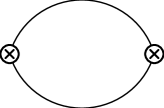
FIG. 1.: Fermion-antifermion propagation graph. The two $\otimes$ create and annihilate a fermion-antifermion pair.

Thus the effective field theory at $\mu=m$ must resum the ${\mathbf{p}}^{2}/2m$ term in the propagator to reproduce the infrared physics of full QCD, and to correctly reproduce the two-loop anomalous dimension. Once the ${\mathbf{p}}^{2}/2m$ term is included in the quark propagator, it is also necessary to perform a multipole expansion and include a quark-antiquark potential [8]. The matching from QCD to an effective theory with potentials is done at the scale $\mu=m$, so the potential in the effective theory at $\mu=m$ depends on $\alpha_{s}(m)$. Since the dominant momenta in the static potential are of order $mv$, one might expect that the relevant coupling is $\alpha_{s}(mv)$, and this is borne out by more detailed studies of the quark static potential [20, 21, 22]. One therefore requires that the potential generated at $\mu=m$ must run in the effective theory below $m$. This running can be implemented by the inclusion of soft gluon modes, with $(E,{\mathbf{p}})\sim(mv,mv)$, the importance of which was pointed out by Greisshammer [15]. Soft gluon modes should be integrated out of NRQCD, since they can never be produced on-shell; nevertheless they must be included in the running between $m$ and $mv$.

A Possible Hierarchies

In addition to the scale $mv$ and $mv^{2}$ the non-perturbative scale $\Lambda_{\rm QCD}$ also plays an important role for real quarkonium. Though $\Lambda_{\rm QCD}$ will not play an important role for the analysis of this paper, some aspects of its power counting are worth emphasizing.

For very large $m$, or equivalently, small $\alpha_{s}(m)$, one is in the regime $\Lambda_{\rm QCD}\ll mv^{2}\ll mv\ll m$, since $\Lambda_{\rm QCD}$ is formally smaller than any power of $\alpha_{s}$. These inequalities are only well satisfied for $t$ quarks; for charmonium and bottomium the situation is closer to $\Lambda_{\rm QCD}\sim mv^{2}$ or $\Lambda_{\rm QCD}\sim mv$, and non-perturbative effects become important. Of course, the apparent independence of $mv$, $mv^{2}$ and $\Lambda_{\rm QCD}$ for a Coulomb system is illusory. The velocity $v$ in a Coulomb bound state is given by solving $v=\alpha_{s}(mv)$,

$$v={4\pi\over b_{0}\ln\left(m^{2}v^{2}/\Lambda_{\rm QCD}^{2}\right)},$$ (7)

where

$$b_{0}=11-{2\over 3}n_{f}$$ (8)

which gives $v=\alpha_{s}(mv)$ as a function of $m/\Lambda_{\rm QCD}$. In Fig. 2,

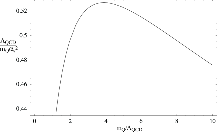
FIG. 2.: Plot of $\Lambda_{\rm QCD}/m\alpha_{s}^{2}(mv)$ as a function of $m/\Lambda_{\rm QCD}$, for $n_{f}=3$.

$\Lambda_{\rm QCD}/m\alpha_{s}^{2}(mv)$ is plotted as a function of $m/\Lambda_{\rm QCD}$, with $v=\alpha_{s}(mv)$. Clearly, for large $m/\Lambda_{\rm QCD}$, one can have $\Lambda_{\rm QCD}\ll mv^{2}\ll mv\ll m$. However, it is not possible to have $\Lambda_{\rm QCD}\gg mv^{2}$. The maximum possible value of $\Lambda_{\rm QCD}/mv^{2}$ is

$${\Lambda_{\rm QCD}\over mv^{2}}={b_{0}\over 2\pi e}=0.53\ \ (\hbox{for }n_{f}=3),$$ (9)

at

$${m\over\Lambda_{\rm QCD}}={eb_{0}\over 2\pi}=3.9,\ v={2\pi\over b_{0}}=0.70\ \ (\hbox{for }n_{f}=3).$$ (10)

[Here $e=2.718$.] (Of course these values should only be taken as illustrative, since if $\Lambda_{\rm QCD}\sim mv^{2}$ the system is no longer Coulombic). For the $J/\Psi$, $m_{c}/\Lambda_{\rm QCD}\sim 3$ and for the $\Upsilon$, $m_{b}/\Lambda_{\rm QCD}\sim 9$ so that $mv^{2}/\Lambda_{\rm QCD}$ is not very different in the two cases.

III The Effective Theory

To construct the effective theory, label the total energy $E$ and momentum $\mathbf{P}$ of the heavy quark by

$${\mathbf{P}=p+k},\qquad E=k^{0},$$ (11)

where the three-vector $\mathbf{p}$ is of the order of the soft scale $mv$, and the four-vector $k$ is of the order of the ultrasoft scale $mv^{2}$. Momentum space of size $mv$ is divided up into boxes of size $mv^{2}$. The location of each box is labeled by $\mathbf{p}$, and the points within a box are labeled by $\mathbf{k}$, as shown in Fig. 3

FIG. 3.: Momentum space of size $mv$ is divided into boxes of size $mv^{2}$. A point in momentum space is labeled by $\mathbf{p}$ and $\mathbf{k}$.

The variable $\mathbf{p}$ is a discrete label, and $\mathbf{k}$ is a continuous label. This procedure was originally used by Georgi for HQET [23], where the four-momentum $p^{\mu}$ was split between $mv^{\mu}$ of order $m$ and the residual momentum $k^{\mu}$ of order $\Lambda_{\rm QCD}$,

$$p^{\mu}=mv^{\mu}+k^{\mu}.$$ (12)

In HQET, the velocity $v$ is a discrete label, and $k$ is a continuous label, so that one sums on $v$ and integrates over $k$ [23]. In our case, we will sum over $\mathbf{p}$ and integrate over $\mathbf{k}$.

The quark field $\psi(x)$ in QCD is replaced by

$$\psi\left(x\right)\to\psi_{\mathbf{p}}\left(x\right).$$ (13)

The label $\mathbf{p}$ represents momenta of order the soft scale $mv$, and (the Fourier transform of) $x$ represents energy and momenta of order the ultrasoft scale $mv^{2}$.

The decomposition Eq. (12) is not unique, since one can redefine $k\to k+q$, $mv\to mv-q$, where $q$ is of order $k$. This redefinition, called reparameterization invariance, leads to constraints on the effective field theory, and relates different orders in the $1/m$ expansion [24]. One can make a similar redefinition here,

$$\mathbf{k}\to\mathbf{k+q},\qquad\mathbf{p}\to\mathbf{p-q},$$ (14)

where $\mathbf{q}$ is of order $mv^{2}$. In terms of fields, this transformation is

$$\psi_{\mathbf{p}}\left(x\right)\to e^{i\mathbf{q\cdot x}}\psi_{\mathbf{p-q}}\left(x\right).$$ (15)

The application of reparameterization invariance to spinors in HQET was subtle, because of the constraint ${\hbox to0.0pt{$v$\hss}/}\psi=\psi$, that projected out the particle component of the spinor. In our case $\psi_{\mathbf{p}}$ is a two-component spinor whose upper and lower components represent the amplitudes to annihilate a quark with spin $\pm 1/2$ along a fixed axis. The transformation Eq. (14) does not affect the spin labels, so the consequences of reparameterization invariance are similar to the case of HQET for spin-zero particles. [Spin would enter if the components of $\psi_{\mathbf{p}}$ represented helicity states.] The basic result is that derivatives on $\psi_{\mathbf{p}}(x)$ should be of the form $i\mathbf{p+\nabla}$ [24].

On-shell gauge fields have energy of order their momentum. One can have propagating gauge fields with energy and momentum of order $mv$ or of order $mv^{2}$, which are referred to as soft and ultrasoft gauge fields, respectively. The gauge fields in the full theory are replaced by two different fields in the effective theory, momentum-dependent gauge fields, $A_{p}^{\mu}(x)$, and momentum-independent gauge fields $A^{\mu}(x)$. The fields $A_{p}^{\mu}(x)$ represent the soft degrees of freedom and $A^{\mu}(x)$ represent the ultrasoft degrees of freedom. The total energy and momentum of the soft gauge fields is

$${\mathbf{P}=p+k},\qquad E=p^{0}+k^{0},$$ (16)

and of the ultrasoft gauge fields is $k^{\mu}$, where $k$ is the Fourier transform of the spacetime argument $x$. Note that soft gauge fields are labeled by a four-vector $p$, whereas quark fields are labeled by a three-vector $\mathbf{p}$. Any other light modes (such as light fermions and ghosts) in the theory must also be divided into soft and ultrasoft fields, as for the gauge fields.

The terms in the NRQCD effective Lagrangian describe the interactions of the soft gauge fields among themselves, and the interaction of two or more soft gauge fields with the fermions. There are no terms that involve the interaction of a fermion with a single soft gauge field, i.e. no vertex of the form $\psi^{\dagger}_{\mathbf{p}^{\prime}}A^{\mu}_{q}\psi_{\mathbf{p}}$, since energy cannot be conserved in the interaction.

The effective Lagrangian for NRQCD can now be written down in terms of the fields $\psi_{\mathbf{p}}$ which annihilate a quark, $\chi_{\mathbf{p}}$ which annihilate an antiquark, $A^{\mu}_{p}$ which annihilate and create soft gluons, and $A^{\mu}$ which annihilate and create ultrasoft gluons. The covariant derivative is $D^{\mu}=\partial^{\mu}+igA^{\mu}=(D^{0},-\mathbf{D})$, so that $D^{0}=\partial^{0}+igA^{0}$, ${\mathbf{D}}={\mathbf{\nabla}}-ig{\mathbf{A}}$, and involves only the ultrasoft photon fields. The effective Lagrangian is gauge invariant under ultrasoft gauge transformations, those in which the gauge parameter varies on a distance scale $1/(mv^{2})$. The full gauge invariance of the original Lagrangian is recovered by combining gauge invariance in the effective theory with reparameterization invariance.

The effective Lagrangian in the center of mass frame is

$${\cal L} = -{1\over 4}F^{\mu\nu}F_{\mu\nu}+\sum_{p}\left|p^{\mu}A^{\nu}_{p}-p^{\nu}A^{\mu}_{p}\right|^{2}+\sum_{\mathbf{p}}\psi_{\mathbf{p}}^{\dagger}\Biggl{\{}iD^{0}-{\left({\bf p}-i{\bf D}\right)^{2}\over 2m}\Biggr{\}}\psi_{\mathbf{p}}$$ (21)

$$-4\pi\alpha_{s}\sum_{q,q^{\prime}\mathbf{p},p^{\prime}}\Biggl{\{}{1\over q^{0}}\psi_{\mathbf{p^{\prime}}}^{\dagger}\left[A^{0}_{q^{\prime}},A^{0}_{q}\right]\psi_{\mathbf{p}}$$

$$+{g^{\nu 0}\left(q^{\prime}-p+p^{\prime}\right)^{\mu}-g^{\mu 0}\left(q-p+p^{\prime}\right)^{\nu}+g^{\mu\nu}\left(q-q^{\prime}\right)^{0}\over\mathbf{\left missing}(p^{\prime}-p\right)^{2}}\psi_{\mathbf{p^{\prime}}}^{\dagger}\left[A^{\nu}_{q^{\prime}},A^{\mu}_{q}\right]\psi_{\mathbf{p}}\Biggr{\}}$$

$$\qquad\qquad+\psi\leftrightarrow\chi,\ T\leftrightarrow\bar{T}$$

$$+\sum_{\mathbf{p},q}{4\pi\alpha_{s}\over\mathbf{\left missing}(p-q\right)^{2}}\psi_{\mathbf{q}}^{\dagger}T^{A}\psi_{\mathbf{p}}\chi_{\mathbf{-q}}^{\dagger}\bar{T}^{A}\chi_{\mathbf{-p}}+\ldots$$

where we have retained the lowest order terms in each sector of the theory. The matrices $T^{A}$ and $\bar{T}^{A}$ are the color matrices for the $\bf 3$ and $\bf\bar{3}$ representations, respectively. The field strength tensor $igF^{\mu\nu}=\left[D^{\mu},D^{\nu}\right]$ is constructed only out of ultrasoft gauge fields. If we were interested in including the effects of light quarks we would need to add new soft and ultrasoft fields for each flavor. The matching at the scale $m$ would then introduce additional non-local four fermion terms involving both the heavy and light quark fields.

In using Eq. (21), it is crucial to expand out the term $\left({\bf p}-i{\bf D}\right)^{2}$. The ${\mathbf{p}}^{2}$ piece is part of the leading order Lagrangian that gives the $\psi_{\mathbf{p}}$ propagator,

$$\psi_{\mathbf{p}}^{\dagger}\Biggl{\{}iD^{0}-{{\bf p}^{2}\over 2m}\Biggr{\}}\psi_{\mathbf{p}},$$ (22)

and the terms involving $\mathbf{D}$ are treated as a perturbation. This is the momentum space equivalent of the multipole expansion written in $x$ space in [8], since the ultrasoft gluons do not transfer three momentum to the quarks. This procedure will be justified when the velocity power counting rules for the Lagrangian are derived.

The QCD Lagrangian contains gauge fixing terms and ghost interactions. It is convenient to quantize the theory in background field gauge. The background fields can be taken to be the ultrasoft modes of the effective theory. The quantum fields represent the quark potential, and the soft modes of the effective theory. The effective Lagrangian is gauge invariant with respect to the ultrasoft modes, and contains the gauge fixing terms of the original theory for the soft modes. One can then gauge fix the ultrasoft gauge fields, to compute loop graphs involving the ultrasoft gauge fields. We will use Feynman gauge for both the soft and ultrasoft modes.

The terms in the effective Lagrangian Eq. (21) are obtained by matching graphs in QCD and the effective theory. The ultrasoft gluon fields $A^{\mu}$ in the effective Lagrangian cannot change the momentum label $\mathbf{p}$ on the fermion lines, so the single-quark terms in $L$ do not change $\mathbf{p}$. The Lagrangian in the single-quark sector is the same as the HQET Lagrangian, as pointed out in Ref. [7]. This relation between the NRQCD and HQET Lagrangians holds even if loop corrections are included. Consider a loop contribution to a term in the single-quark sector of the effective theory, such as that shown in Fig. 4.

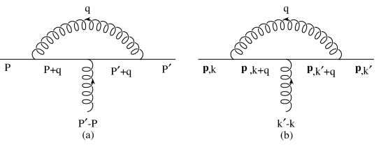
FIG. 4.: One loop vertex correction in the full theory and effective theory. The momenta are related by $P=p+k$, $P^{\prime}=p+k^{\prime}$.

In the effective theory, the incoming and outgoing momenta of the quark, $P$ and $P^{\prime}$ respectively, are broken up into a soft piece $\mathbf{p}$ and an ultrasoft piece $k,k^{\prime}$. The soft label $\mathbf{p}$ must be the same on the incoming and outgoing lines, since the ultrasoft gluons do not change $\mathbf{p}$, so the momentum transfer in the effective theory is $k^{\prime}-k=P^{\prime}-P$. The matching condition can be computed as the difference between Fig. 4(a) and (b), expanded in a power series in $1/m$. The full-theory computation is given by computing Fig. 4(a) on-shell, and expanding in powers of the external momenta over $m$. The effective theory contribution is given by evaluating Fig. 4(b) on-shell. The on-shell condition in the effective theory is $k^{0}={\mathbf{p}}^{2}/2m$. The intermediate fermion propagator

$${1\over k^{0}+q^{0}-{\mathbf{p}}^{2}/2m+i\epsilon}$$ (23)

is equal to

$${1\over q^{0}+i\epsilon}$$ (24)

when the on-shell condition is used. The Feynman rules Eq. (24) are precisely those that would be used to match from QCD to HQET, and are known not to violate the $1/m$ power counting in the effective theory. Thus the couplings of the ultrasoft gluons in the single-quark sector are precisely those in HQET. This was the procedure used to compute the HQET and NRQCD Lagrangians at one-loop in Ref [7].

The Coulomb potential can scatter quark states from one value of $\mathbf{p}$ to another. These effects are explicitly included in the two-body terms in $L$. The Coulomb potential is usually thought of as a nonlocal two-body operator. However, because of the use of the extra label $\mathbf{p}$, the Coulomb potential,

$${4\pi\alpha\over\mathbf{\left missing}(p-q\right)^{2}}\psi_{\mathbf{q}}^{\dagger}T^{A}\left(x\right)\psi_{\mathbf{p}}\left(x\right)\chi_{\mathbf{-q}}^{\dagger}\left(x\right)\bar{T}^{A}\chi_{\mathbf{-p}}\left(x\right)$$ (25)

is local, and manifestly gauge invariant. The Coulomb potential is obtained as the value of Fig. 5 evaluated in the full theory.

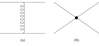
FIG. 5.: The Coulomb potential in the full theory, (a), is given by a local two-quark operator (b) in the effective theory.

The Coulomb potential is proportional to the Casimir $T^{A}\bar{T}^{A}$, and gives an attractive interaction in the color singlet channel and a repulsive interaction in the color octet channel.

The leading terms involving the soft gluons are given by matching the Compton scattering graphs Figs. 6(a,b,c) in the full theory to the local operator Fig. 6(d) in the effective theory.

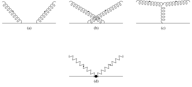
FIG. 6.: The Compton scattering graphs (a,b,c) match on to a local operator (d) in the effective theory. Soft gluon modes are denoted by a zigzag line.

Soft gluons have energy and momenta of order $mv$, whereas the quarks $\psi_{\mathbf{p}}$ have energies of order $mv^{2}$ and momenta of order $mv$. The intermediate quark in Fig. 6(a,b) is off-shell, and the Compton scattering graph in the full-theory can be replaced by a local vertex in the effective theory, as shown in the figure. The intermediate gluon in Fig. 6(c) is also off-shell, since energy cannot be transferred from the external gluons to the quark line. Thus the interaction in Fig. 6(c) can also be represented by a local vertex in the effective theory. The leading order soft interaction vanishes for QED. We will comment on this in Sec. V. Loop graphs involving the soft interaction of Fig. 6(d) are part of the running potential in the effective theory.

The Lagrangian Eq. (21) is similar to the pNRQCD Lagrangian constructed by Pineda and Soto in Ref. [25], but there are a few important differences. The Lagrangian is given by matching to QCD at the scale $\mu=m$, rather than at the scale $\mu=mv$. The Lagrangian also contains explicit soft modes. Soft modes are necessary to reproduce the running potential in the effective theory. Finally, the Coulomb potential is constructed using a $\mathbf{p}$-dependent, but local in $\mathbf{x}$ two-body operator, instead of a two-body operator nonlocal in $\mathbf{x}$. The use of $\mathbf{p}$-dependent fields is the momentum space analog of the multipole expansion, and simplifies the discussion of gauge invariance, particularly in the non-Abelian case.

A Power Counting in the Lagrangian

The NRQCD effective Lagrangian can be used to compute processes to a given order in the velocity $v$. To determine the order in $v$ of a given diagram, it is useful to have a velocity power counting scheme, and we will use the one in Table I.

TABLE I.: Velocity counting rules for the effective theory. The electric and magnetic fields are those constructed out of the ultrasoft gauge potential $A^{\mu}$.

${\mathbf{p}}$	$v$
$\psi,\ \chi$	$v^{3/2}$
$A_{p}^{\mu}$	$v$
$D^{0}$	$v^{2}$
$\mathbf{D}$	$v^{2}$
$A^{\mu}$	$v^{2}$
${\mathbf{E}}$	$v^{4}$
${\mathbf{B}}$	$v^{4}$

This velocity power counting scheme differs somewhat from that in BBL, since we have separated the gluon field into soft and ultrasoft modes, and the Coulomb interaction. The order in $v$ of the soft gluons modes $A_{p}$ is irrelevant, since they cannot appear as external states in the processes we are considering. The final power counting formula for graphs we will derive in Eq. (45) holds regardless of the order in $v$ chosen for $A_{p}$. The lowest dimension operator in the zero-quark sector of the Lagrange density is the gauge kinetic energy, which is of order $v^{8}$. All the terms in the field strength tensor $F^{\mu\nu}$ are of the same order in $v$, since $D^{\mu}$ and $A^{\mu}$ are both of order $v^{2}$.

The lowest dimension terms in the one-quark sector are

$$\psi_{\mathbf{p}}^{\dagger}\left(x\right)\left\{iD^{0}-{{\bf p}^{2}\over 2m}\right\}\psi_{\mathbf{p}}\left(x\right)$$ (26)

which are of order $v^{5}$. The lowest order Lagrangian Eq. (26) must be used to determine the $\psi_{\mathbf{p}}$ propagator. Terms that involve the covariant derivative $\mathbf{D}$ are of higher order than $v^{5}$. For example,

$$\psi_{\mathbf{p}}^{\dagger}{{\mathbf{p}\cdot D}\over m}\psi_{\mathbf{p}}$$ (27)

is of order $v^{6}$, and must be treated as a perturbation in the effective theory. Each replacement of $\mathbf{p}$ by $\mathbf{D}$ increases the order in $v$ by one.

The lowest dimension operator in the two-quark sector is the Coulomb interaction. Each quark field is of order $v^{3/2}$ and $1/({\mathbf{p}-q})^{2}$ is of order $1/v^{2}$, so the Coulomb interaction is of order $\alpha_{s}v^{4}$.

The lowest dimension terms that involve soft gluons are of order $\alpha_{s}v^{4}$. Consider, for example,

$$-4\pi\alpha_{s}\sum_{q,q^{\prime}\mathbf{p},p^{\prime}}{1\over q^{0}}\psi_{\mathbf{p^{\prime}}}^{\dagger}\left[A^{0}_{q^{\prime}},A^{0}_{q}\right]\psi_{\mathbf{p}}.$$ (28)

The two $\psi_{\mathbf{p}}$ fields are of order $v^{3}$, the two $A^{0}_{q}$ fields are of order $v^{2}$, and $1/q^{0}$ is of order $1/v$, so the vertex is of order $\alpha_{s}v^{4}$.

B Loop Graphs

The computation of loop graphs using the effective Lagrangian Eq. (21) involves some subtleties. There are three kinds of loops, which we will refer to as ultrasoft, potential and soft, respectively. We will determine the dominant momentum region for each graph by studying the pole structure of the diagram, which is what determines the behavior of the graph in the $\overline{\rm MS}$ scheme.

Consider graphs in the effective theory that involve only a single fermion line, such as Fig. 4(b). The internal fermion propagators are given by the lowest order term in the one-fermion sector, Eq. (23). These terms depend only on the soft momentum $\mathbf{p}$, and not on the ultrasoft momentum $\mathbf{k}$ carried by the gluon lines. Thus the two fermion propagators in Fig. 4(b) are

$${1\over k^{0}+q^{0}-{\bf p}^{2}/2m},\ \hbox{and}\ {1\over k^{\prime 0}+q^{0}-{\bf p}^{2}/2m},$$ (29)

respectively. These propagators do not depend on the space part of the loop momentum $\mathbf{q}$, but they do depend on $m$. The propagators have poles at energies of order ${\bf p}^{2}/2m$ or $k^{0}$. The pole positions are set by the external gluon and quark energies, and also by ${\bf p}^{2}/2m$, which depends on the quark momentum. The fact that the energy poles are determined by the momentum (and vice versa), is important, because it relates the soft and ultrasoft scales. We will refer to a typical external quark energy as of the order of the ultrasoft scale $\mu_{\rm U}$, and a typical external quark momentum as of the order of the soft scale $\mu_{\rm S}$. Then loop graphs in the one-fermion sector have poles at energies of order $\mu_{\rm U}$ and $\mu_{\rm S}^{2}/m$. The gauge boson propagator is $1/[(q^{0})^{2}-{\mathbf{q}}^{2}]$, so the typical momenta in the loop are of the same order as the gluon energy, $\mathbf{q}\sim q^{0}$. Loop graphs such as Fig. 4(b) in which the ultrasoft momentum $q$ is integrated over will be referred to as ultrasoft loops, and when evaluated in dimensional regularization, are dominated by energy and momenta of order $\mu_{\rm U}$ or $\mu_{\rm S}^{2}/m$.

The use of ${\bf p}^{2}/2m$ rather than $\left({\bf p+q}\right)^{2}/(2m)$ in the propagators removes the problem of the breakdown of the effective theory due to poles of order $m$ in loop graphs. The power counting scheme of Table I in which $\mathbf{p}$ is of order $mv$, but $\mathbf{q}$ is of order $mv^{2}$ requires that $\left({\mathbf{p}+q}\right)^{2}$ be expanded as $\mathbf{p}^{2}+2p\cdot q+q^{2}$, with $\bf p^{2}$ included in the fermion propagator, and the higher order terms $\mathbf{2}p\cdot q+q^{2}$ treated as vertex insertions.

Consider a graph that involves a potential loop, such as the one-loop correction to Coulomb scattering. The graph is shown as Fig. 7(a) in the full theory, and as Fig. 7(b) in the effective theory.

FIG. 7.: One loop correction to Coulomb Scattering in the full and effective theories.

The external fermions have energy $E$ and momenta $\pm\mathbf{p},p^{\prime}$. In the effective theory, the external fermions are labeled by the soft momentum $\pm\mathbf{p},p^{\prime}$, and the ultrasoft momentum $(E,0)$. The intermediate fermions in the effective theory have soft momentum $\pm q$, and ultrasoft momentum $(E,0)\pm k$. The graph in the effective theory is

$$\propto\sum_{\mathbf{q}}\int d^{4}k{1\over\mathbf{(}p-q)^{2}}\ {1\over\mathbf{(}p^{\prime}-q)^{2}}\ {1\over k^{0}+E-{\mathbf{q}}^{2}/2m}\ {1\over-k^{0}+E-{\mathbf{q}}^{2}/2m}.$$ (30)

There is an integral over the ultrasoft energy $k^{0}$, the ultrasoft momentum $\mathbf{k}$, and a sum over the soft momentum $\mathbf{q}$. Recall the decomposition of momentum space shown in Fig. 3. Summing over $\mathbf{q}$ and integrating over $\mathbf{k}$ is equivalent to integrating over the entire momentum space. Thus one can replace Eq. (30) by

$$\int d^{4}q{1\over\mathbf{(}p-q)^{2}}{1\over\mathbf{(}p^{\prime}-q)^{2}}{1\over q^{0}+E-{\mathbf{q}}^{2}/2m}{1\over-q^{0}+E-{\mathbf{q}}^{2}/2m},$$ (31)

where

$$dk^{0}\to dq^{0},\qquad\sum_{\mathbf{q}}\int d{\mathbf{k}}\to\int d{\mathbf{q}}.$$ (32)

The loop graph is dominated by $q^{0}\sim E$, and ${\mathbf{q}}\sim\sqrt{mE}$, which are ultrasoft, and soft, respectively. This is consistent with the picture that $q^{0}$ ranges over a box of size $mv^{2}$ and $\mathbf{q}$ over a box of size $mv$. It again shows that one cannot treat the soft and ultrasoft scales as independent of each other; they are related by $\hbox{(soft)}^{2}\sim\hbox{ultrasoft}\times m$.

Finally, consider a graph such as Fig. 8 that involves a soft loop.

FIG. 8.: One loop graph involving the soft gauge fields. This graph contributes to the running potential in the effective theory.

It gives a contribution of the form

$$\propto\sum_{q}\int d^{4}k{1\over\mathbf{(}p-p^{\prime})^{2}}\ {1\over\mathbf{(}p-p^{\prime})^{2}}\ {1\over\left(q^{0}\right)^{2}-{\mathbf{q}}^{2}}\ {1\over\left(q^{0}\right)^{2}-\left({\mathbf{q}+p-p^{\prime}}\right)^{2}},$$ (33)

where we have used the last interaction in Eq. (21) for the soft vertices. The sum on $q$ is over a four-vector. As for potential loops, one can make the replacement

$$\sum_{q}\int d^{4}{k}\to\int d^{4}{q},$$ (34)

where the replacement must be done for all four components of $q$, since soft gluons carry a four-vector label $q$. It is straightforward to see that Eq. (33) is dominated by $q^{0}$ and $q$ of order $mv$, which is consistent with using the replacement Eq. (32) for all four components of $q$.

C Power Counting Formula for Loop Graphs

It is now straightforward to derive a power counting rule for an arbitrary graph in NRQCD. A given graph has $L_{U}$ ultrasoft loops, $L_{P}$ potential loops, and $L_{S}$ soft loops. These can be determined from the structure of the diagram in a systematic way. The total number of loops is $L_{U}+L_{P}+L_{S}$. Now delete all the ultrasoft lines from the graph. The remaining number of loops is $L_{P}+L_{S}$. Finally, delete all quark lines from the diagram. The remaining number of loops is $L_{S}$. An example of loop counting is shown in Fig. 9.

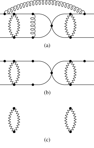
FIG. 9.: An example of counting ultrasoft, potential and soft loops and vertices. Graph (a) has 9 vertices and 6 loops. Deleting all ultrasoft lines gives graph (b), which has 9 vertices and 4 loops. Deleting all fermion lines from graph (b) gives graph (c), with 4 vertices and 2 loops, which is the number of soft vertices and loops. There are 5 potential vertices and 2 potential loops (the difference between (b) and (c)), and 4 ultrasoft vertices and 2 ultrasoft loops (the difference between (a) and (b)). The graph (c) has two connected soft components, $N_{S}=2$.

Let $V_{k}$ denote the number of vertices of order $v^{k}$ in a given graph. For example, $\psi_{\mathbf{p}}^{\dagger}iD^{0}\psi_{\mathbf{p}}$ is a vertex of type $V_{5}$, since it is a one-fermion vertex of order $v^{5}$. It is convenient to break up the vertices into ultrasoft, $V^{(U)}_{k}$, potential $V^{(P)}_{k}$ and soft $V^{(S)}_{k}$. The ultrasoft vertices $V^{(U)}_{k}$ are those vertices in $V_{k}$ that involve only ultrasoft fields, the potential vertices $V^{(P)}_{k}$ are those with at least one fermion field and no soft fields. The soft vertices $V^{(S)}_{k}$ involve at least one soft field. An example of vertex counting is shown in Fig. 9.

A diagram is of order $v^{\delta}$, where

$$\delta=\sum_{k}k\left[V^{(U)}_{k}+V^{(P)}_{k}+V^{(S)}_{k}\right]-5I_{F}-4I_{S}-8I_{U}+8L_{U}+5L_{P}+4L_{S}.$$ (35)

The first term simply adds up the powers in $v$ of all the vertices. Each internal quark line eliminates two $\psi_{\mathbf{p}}$ fields, and gives a factor of the fermion propagator $1/(E-{\bf p}^{2}/2m)$, which give a net factor of $1/(v^{3}v^{2})=v^{-5}$. This gives the term $-5I_{F}$, where $I_{F}$ is the number of internal fermion lines. Each internal soft line eliminates two $A_{p}$ fields, and gives a factor of the gauge propagator $1/((p^{0})^{2}-{\bf p}^{2})$, which gives a net factor of $1/(v^{2}v^{2})=v^{-4}$. This gives the term $-4I_{S}$, where $I_{S}$ is the number of internal soft lines. Each internal ultrasoft line eliminates two $A^{\mu}$ fields, and gives a factor of the gauge propagator $1/((k^{0})^{2}-{\bf k}^{2})$, which gives a net factor of $1/(v^{4}v^{4})=v^{-8}$. This gives the term $-8I_{U}$, where $I_{U}$ is the number of internal ultrasoft lines.

Ultrasoft loops are dominated by energy and momentum of order $mv^{2}$, and give give a factor of $v^{2}$ for each integral, so that one gets a factor of $v^{8}$ for each loop. Potential loops are dominated by energy of order $mv^{2}$ and momentum of order $mv$, and give a factor of $v^{2}$ for each time integration, and $v$ for each space integration, for a net factor of $v^{5}$ per loop. Soft loops are dominated by energy and momentum of order $mv$, and give a factor of $v$ for each integration, for a net factor of $v^{4}$ for each loop. These contributions give the $8L_{U}+5L_{P}+4L_{S}$ term in Eq. (35).

The identity

$$\sum_{k,n}\left[V^{(U)}_{k}+V^{(P)}_{k}+V^{(S)}_{k}\right]-I_{F}-I_{S}-I_{U}+L_{U}+L_{P}+L_{S}=1,$$ (36)

is the usual relation that the Euler character of a connected graph is unity. An analogous relation holds for the graph with all ultrasoft lines removed. We will assume that the graph remains connected when ultrasoft lines are removed, which is true for any process in which momentum of order $mv$ is transferred between the two fermion lines. The relation for the graph with ultrasoft lines removed is

$$\sum_{k}\left[V^{(P)}_{k}+V^{(S)}_{k}\right]-I_{F}-I_{S}+L_{P}+L_{S}=1.$$ (37)

For $I_{F}$ to be equal in the two relations Eq. (36) and (37), it is important that one not erase vertices where the gluons couple to the fermions (see Fig. 9), so the total number of vertices is given by $V^{(P)}_{k}+V^{(S)}_{k}$. Finally, one has the Euler character relation for the graph with all ultrasoft and fermion lines removed,

$$\sum_{k}V^{(S)}_{k}-I_{S}+L_{S}=N_{S},$$ (38)

where $N_{S}$ is the number of connected components in the soft graph.

Eliminating $I_{U}$, $I_{F}$ and $L_{S}$ between Eqs. (35–38) gives the result

$$\delta=5+\sum_{k}\left[(k-8)V^{(U)}_{k}+(k-5)V^{(P)}_{k}+(k-4)V^{(S)}_{k}\right]-N_{S}.$$ (39)

A given soft vertex in the Lagrange density has the generic form

$$\left(\psi_{\mathbf{p}}\right)^{a}\left(A_{q}\right)^{b}\left(A^{\mu}\right)^{c}{\mathbf{p}}^{d}\left(D\right)^{e}\left({1\over m}\right)^{f},$$ (40)

where $\psi_{\mathbf{p}}$ represents any quark or antiquark fields or their conjugates. The term Eq. (40) has dimension four,

$$4={3\over 2}a+b+c+d+e-f,$$ (41)

and is of order $v^{k}$, where

$$k={3\over 2}a+b+2c+d+2e.$$ (42)

Subtracting these two relations gives

$$k-4=c+e+f.$$ (43)

The vertex can only have positive powers of $D$, $A^{\mu}$, and $1/m$, so $c+e+f\geq 0$. [Note that $d$ need not be positive.] For a soft vertex, let $\sigma=c+e+f\geq 0$. Label the soft vertices $V^{(S)}_{k}$ by the values of $b$ and $\sigma$, so that they are denoted by $V^{(S)}_{b,\sigma}$, where $k=4+\sigma$. Then one finds

$$\sum_{k}(k-4)V^{(S)}_{k}=\sum_{b,\sigma}\sigma V^{(S)}_{b,\sigma}.$$ (44)

Substituting this result into Eq. (39) gives the power counting formula

$$\delta=5+\sum_{k}\left[(k-8)V^{(U)}_{k}+(k-5)V^{(P)}_{k}\right]+\sum_{\sigma}\sigma V^{(S)}_{b,\sigma}-N_{S}.$$ (45)

This is an important result. All terms in the zero-fermion sector have $k\geq 8$, and in the nonzero fermion sector have $\sigma\geq 0$. Thus the contributions of $(k-8)V^{(U)}_{k}$, and $\sigma V^{(S)}_{b,\sigma}$ are each positive. There can be negative powers of $v$ from both soft and potential exchange, but these come with compensating factors of $\alpha_{s}$. The Coulomb interaction is $k=4$ vertex in $V^{(P)}$, but is of order $\alpha_{s}$. Iterating the Coulomb interaction $n$ times produces terms of order $(\alpha_{s}/v)^{n}$, so for $v\sim\alpha_{s}$, the Coulomb interaction must be summed to all orders. The $N_{S}$ term is negative, but each soft component must contain at least one power of $\alpha_{s}$.

As an example of Eq. (39), consider the electron self-energy diagram Fig. 10

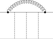
FIG. 10.: Graph contributing to the Lamb shift. The dot represents a $\mathbf{p}\cdot A$ interaction.

which produces the Lamb shift. The graph contains two $\mathbf{p}\cdot A$ vertices, each of which is of order $v^{6}$, and one ultrasoft loop, so the net power is $\delta=5+(6-5)\times 2=7$. The graph has a factor of $\alpha_{s}$ from the two gauge couplings, and so is of order $\alpha_{s}v^{7}$ compared to the leading term in the single-fermion sector (which is of order $v^{5}$), i.e. it is of relative order $\alpha_{s}v^{2}$. Similarly the soft loop graph in Fig. 8 has $\sigma=0$, and $N_{S}=1$, and so is of order $\alpha_{s}^{2}v^{4}$. This is the same order in $v$, but one higher order in $\alpha_{s}$ than the Coulomb interaction.

IV Velocity Renormalization Group Equation

Loop diagrams in the effective theory can be divergent, and the effective theory is renormalized using the $\overline{\rm MS}$ scheme. A scale parameter $\mu_{\rm U}$ is introduced when one analytically continues the Lagrangian from four to $D=4-2\epsilon$ dimensions, as in conventional dimensional regularization of gauge theories. There is a subtlety in the use of dimensional regularization in NRQCD. In evaluating loop graphs with potential loops, we made the replacement Eq. (32). In $D$ dimensions, the relation should read

$$dk^{0}\to dq^{0},\qquad\sum_{\mathbf{q}}\int d^{D-1}{\mathbf{k}}\to\left({\mu_{\rm S}\over\mu_{\rm U}}\right)^{4-D}\int d^{D-1}{\mathbf{q}}.$$ (46)

The factor of $\left({\mu_{\rm S}/\mu_{\rm U}}\right)^{4-D}$ is needed to ensure the correct dimensionality on the two sides of Eq. (46). The integral over $d{\mathbf{k}}$ is over a volume of the order of $\mu_{\rm U}^{D-1}$, since the typical range of integration is of order $\mu_{\rm U}$. The integral over $d{\mathbf{q}}$ is over a volume of the order of $\mu_{\rm S}^{D-1}$, since the range of integration is of order $\mu_{\rm S}$. The number of terms in the sum on ${\mathbf{q}}$ on the left-hand side of Eq. (46) is the ratio of the two volumes in four dimensions, $\left({\mu_{\rm S}/\mu_{\rm U}}\right)^{3}$. Away from four dimensions, this number does not properly account for the momentum space volumes on the two sides of Eq. (46), and the additional factor of $\left({\mu_{\rm S}/\mu_{\rm U}}\right)^{D-4}$ is needed. The mismatch of dimensions in $D\not=4$ occurs only for the space part of the integral. The factor above is correct when the NRQCD integrals are done in the conventional way, by first doing the $k^{0}$ integral using the method of residues disregarding the contour at infinity, followed by the $\mathbf{k}$ integral in $3-2\epsilon$ dimensions. Similarly, for soft loops Eq. (34) should be replaced by

$$\sum_{q}\int d^{D}{k}\to\left({\mu_{\rm S}\over\mu_{\rm U}}\right)^{4-D}\int d^{D}{q}.$$ (47)

The effective theory renormalized in the $\overline{\rm MS}$ scheme has two $\mu$ parameters, $\mu_{\rm S}$ and $\mu_{\rm U}$. However, the two parameters are not independent, since the soft and ultrasoft scales are related, $\mu_{\rm S}^{2}=m\mu_{\rm U}$. It is better to think of the parameters as $\mu_{\rm S}=m\nu$ and $\mu_{\rm U}=m\nu^{2}$, where $\nu$ is the subtraction point velocity. One can now derive a new kind of renormalization group equation for the effective theory, since the bare theory is independent of the subtraction velocity $\nu$. This velocity renormalization group equation can be used to scale the coefficients in the effective theory from the matching scale $\mu_{\rm S}=m$, $\mu_{\rm U}=m$ to $\mu_{\rm S}=mv$, $\mu_{\rm U}=mv^{2}$, i.e. from $\nu=1$ to $\nu=v$.

The velocity renormalization group equation addresses an important point about the effective theory, the simultaneous existence of two related scales $\mu_{\rm S}$ and $\mu_{\rm U}$. Loop graphs involving gluon loops will typically have logarithms of the form $\ln\mu/E$, where $E\sim mv^{2}$ is the typical photon energy. The scale $\mu$ is equal to $\mu_{\rm U}$, since $\mu_{\rm U}$ is the scale parameter introduced in $D$ dimensions. Loop graphs containing four-fermion terms, (the potential and soft loop graphs discussed earlier), typically have logarithms of the form $\ln\mu/\sqrt{mE}$ or $\ln\mu/{\mathbf{p}}$. These graphs use the replacement Eq. (46), and so have have a factor of

$$\left({\mu_{\rm S}\over\mu_{\rm U}}\right)^{2\epsilon}\mu_{\rm U}^{2\epsilon}=\mu_{\rm S}^{2\epsilon}$$ (48)

for each loop, where the first factor is from Eq. (46), and the second factor is the conventional factor for each loop in dimensional regularization. Thus in potential and soft loops, logarithms are of the form $\ln\mu_{\rm S}/\sqrt{mE}$ or $\ln\mu_{\rm S}/{\mathbf{p}}$. The radiation and potential logarithms are

$$\ln{\mu_{\rm U}\over E}=\ln{m\nu^{2}\over mv^{2}},\qquad\ln{\mu_{\rm S}\over\sqrt{mE}}=\ln{m\nu\over mv}.$$ (49)

The choice of renormalization point $\nu=v$ ensures that both logarithms are simultaneously small. Thus using the velocity renormalization group equation from $\nu=1$ to $\nu=v$ simultaneously sums the logarithms involving the soft and ultrasoft scales. The velocity renormalization group equation is the $\overline{\rm MS}$ equivalent of using an energy cutoff $m\nu^{2}$ and a momentum cutoff $m\nu$ in a hard cutoff scheme. The VRG allows one to have a static potential with an effective coupling constant $\alpha_{s}(m\nu)$, and radiation corrections with an effective coupling constant $\alpha_{s}(m\nu^{2})$.

In a conventional renormalization group approach, one would scale the effective theory from $\mu=m$ to $\mu=mv$, and then down to $\mu=mv^{2}$. The VRG differs from this in an important way, because it uses a subtraction velocity rather than a subtraction scale. Scaling the theory from $\nu=1$ to $\nu=v$ is equivalent to simultaneously scaling potential and soft graphs from $m$ to $mv$, and radiation graphs from $m$ to $mv^{2}$. The scale $mv$ and $mv^{2}$ are coupled in the theory, and this coupling of scales is better treated using a subtraction velocity rather than a subtraction scale.

V Examples

The formalism we have developed will be applied to three illustrative examples in this section, the one-loop correction to the static potential, integrating out a heavy fermion, and the two-loop anomalous dimension of the production current [10, 11].

A Box Graph and the Static Potential

The first example we consider is the renormalization of the static potential at one-loop. At tree-level, the fermion-fermion scattering amplitude is reproduced in the effective theory by a local operator, the Coulomb vertex in Eq. (21). At one-loop, the QCD diagrams that contribute are shown in Table II above the horizontal line, and the graphs in the effective theory are shown below the horizontal line.

TABLE II.: One-loop correction to quark-antiquark scattering. The color factors listed in the table are for the color singlet channel. The column labeled QCD gives the contribution of the graph evaluated in QCD in the $\overline{\rm MS}$ scheme in Feynman gauge, from Titard and Yndurain [26, 27]. Only the logarithmic contributions are given. $\lambda$ is a gluon mass used as an infrared regulator, $k$ is the momentum transfer, and $\mu$ is the scale parameter of dimensional regularization. The gluon vacuum polarization graph includes the contribution from the ghost loop. The column labeled HQET gives the contributions of the diagrams in HQET, where $m\to\infty$. The breakup of the total diagram into soft and ultrasoft contributions is given in the last two columns. The two diagrams below the horizontal line are the contributions to quark-antiquark scattering in the effective theory. The complete set of ultrasoft diagrams is show in Fig. 11.

$\displaystyle\begin{array}[]{lc|cc|cc}\hbox{Diagram}&\hbox{Color Factor}&\hbox{QCD}&\hbox{HQET}&\hbox{Soft}&\hbox{Ultrasoft}\\ \hline\cr\hline\cr&&&&&\\ \lower 15.0pt\hbox{\epsfbox{9911_fdb1.eps}}&C_{F}&2\ln{\lambda\over k}&2\ln{\lambda\over k}&-2\ln{k\over\mu}&2\ln{\lambda\over\mu}\\ &&&&&\\ \lower 15.0pt\hbox{\epsfbox{9911_fdb2.eps}}&\left(C_{F}-{1\over 2}C_{A}\right)&-2\ln{\lambda\over k}&-2\ln{\lambda\over k}&2\ln{k\over\mu}&-2\ln{\lambda\over\mu}\\ &&&&&\\ \lower 15.0pt\hbox{\epsfbox{9911_fdb5.eps}}&C_{F}&-\ln{\mu\lambda^{2}\over m^{3}}&-2\ln{\lambda\over\mu}&0&-2\ln{\lambda\over\mu}\\ &&&&&\\ \lower 15.0pt\hbox{\epsfbox{9911_fdb3.eps}}&\left(C_{F}-{1\over 2}C_{A}\right)&\ln{\mu\lambda^{2}\over m^{3}}&2\ln{\lambda\over\mu}&0&2\ln{\lambda\over\mu}\\ &&&&&\\ \lower 15.0pt\hbox{\epsfbox{9911_fdb4.eps}}&C_{A}&{3\over 2}\ln{\mu\over m}&0&0&0\\ &&&&&\\ \lower 20.0pt\hbox{\epsfbox{9911_fdb6.eps}}&C_{A}&-{5\over 6}\ln{k\over\mu}&-{5\over 6}\ln{k\over\mu}&-{5\over 6}\ln{k\over\mu}&0\\ &&&&&\\ \hline\cr&&&&&\\ \lower 20.0pt\hbox{\epsfbox{9911_fd8.eps}}&C_{A}&&&-{11\over 6}\ln{k\over\mu}&\\ &&&&&\\ \lower 18.0pt\hbox{\epsfbox{9911_fdb7.eps}}&&&&&0\end{array}$

The sum of the QCD diagrams gives the net one-loop contribution to the static potential (in the color singlet channel),

$$V({\mathbf{k}})=-{4\pi\alpha_{s}(\mu)C_{F}\over\left|\mathbf{k}\right|^{2}}\left[1-C_{A}{11\over 6}{\alpha_{s}(\mu)\over\pi}\ln{k\over\mu}\right],$$ (50)

where only the logarithmic term has been retained. This gives the well-known result that the potential can be rewritten as

$$V({\mathbf{k}})={4\pi\alpha_{s}(\left|\mathbf{k}\right|)\over\left|\mathbf{k}\right|^{2}}T\cdot\bar{T},$$ (51)

where $T\cdot\bar{T}=-C_{F}$ in the color singlet channel.

The box graph (the first diagram in Table II) was computed using the threshold expansion by Beneke and Smirnov [4], and it is interesting to see how the effective field theory reproduces the various contributions. The hard part of the box graph is the matching condition between QCD and NRQCD, i.e. a local two-fermion operator in the effective Lagrangian, and is also equal to the difference between the graphs computed in QCD and HQET. The potential part of the box graph is reproduced in the effective theory by the one-loop contribution from the iteration of two Coulomb interactions Fig. 7. The HQET value of the box diagram, $2C_{F}\ln\lambda/k$, is both infrared and ultraviolet finite if a gluon mass $\lambda$ is introduced as an infrared regulator. This total contribution is split, in the the threshold expansion, into an infrared divergent soft contribution $2C_{F}\ln\mu/k$, and an ultraviolet divergent ultrasoft contribution $2C_{F}\ln\lambda/\mu$. The sum of the soft and ultrasoft contributions has no $1/\epsilon$ pole, since the ultraviolet and infrared divergences cancel.

The ultrasoft contribution vanishes in the full and effective theories, if the infrared divergence is regulated by dimensional regularization. The non-trivial contribution is the soft part of the box graph. The importance of this contribution was pointed out by Griesshammer [15], who argued that one needed to introduce soft gauge fields, as well as soft quark fields. In our approach, the soft part of the box graph is reproduced in the effective theory by the loop graph shown in Fig. 8, where the interaction vertex is from the last two lines of Eq. (21). It is not necessary to introduce soft quark fields, as advocated by Griesshammer.

In QED, the soft part of the box and crossed-box graph cancel. This is consistent with the effective Lagrangian Eq. (21), where the soft interaction vertex vanishes for QED. In QED, the soft modes can be integrated out directly at $\nu=1$, and replaced by local operators at the scale $\mu=m$. This approach does not resum the logarithms of $v$ in the potential (which are absent for QED), and so is not a satisfactory procedure for QCD.

The effective theory correctly reproduces the soft and ultrasoft contributions to the static potential. The soft vertex in Fig. 8 is computed from the Compton scattering graphs in Fig. 6. Fig. 8 reproduces the sum of the soft part of the box, vertex and vacuum polarization corrections to fermion-fermion scattering. We have seen that the soft vertex is proportional to the commutator of two gauge fields, so the soft graph Fig. 8 is proportional to $C_{A}$. This automatically implements the cancellation between the various $C_{F}$ contributions to quark-antiquark scattering in the full QCD calculation. An explicit computation of Fig. 8 gives the contribution

$$-{\left(4\pi\alpha_{s}T\cdot\bar{T}\right)\over\left|\mathbf{k}\right|^{2}}{\alpha_{s}\over\pi}C_{A}\left(1+{5\over 6}\right)\ln{k\over\mu_{\rm S}}$$ (52)

to the scattering potential, where the first term (1) is an infrared divergent contribution, and the second (5/6) is an ultraviolet divergent contribution. Note that the soft graph is infrared divergent even if a gluon mass is used as an infrared regulator. The infrared divergent contribution of Eq. (52) is converted to an ultraviolet divergent contribution if tadpole graphs are included. Equation (52) agrees with the sum of the soft contributions listed in Table II.

The ultrasoft contributions in the QCD theory add up to zero. The ultrasoft contributions in the effective theory are the renormalization of the local four-fermion quark-antiquark potential, shown in Fig. 11.

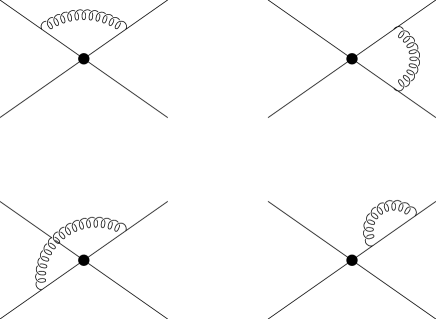
FIG. 11.: Renormalization of the four-quark operator representing the quark-antiquark potential by ultrasoft gluons.

Each graph is ultraviolet divergent, and proportional to $\ln\mu_{\rm U}/k$. The sum of all the graphs is zero, in both the singlet and octet channels. In the effective theory, ultrasoft radiative corrections do not renormalize the quark-antiquark potential. They do, however, cause mixing between the leading order potential, and corrections to the potential suppressed by powers of $1/m$.

The quark-antiquark potential is VRG invariant. This implies that the coupling $\alpha_{s}$ of the soft gluons must satisfy a $\beta$-function equation, where the $\beta$-function for the VRG is the same as the conventional one, since $\mu_{\rm S}=m\nu$, so that $\mu_{\rm S}d/d\mu_{\rm S}=\nu d/d\nu$. In other words, the quark-antiquark potential takes the form Eq. (50), with the coupling constant renormalized at the soft scale $\mu=\mu_{\rm S}=m\nu$. Choosing $m\nu=\left|\mathbf{k}\right|$ sums the leading logarithms, and gives Eq. (51).

The effective theory has performed an interesting rearrangement of the terms in the radiative correction to the static potential, compared with those in the corresponding HQET computation in Feynman gauge. In the HQET computation, the vertex and wavefunction renormalization graphs contribute $-C_{A}\ln k/\mu$, and the vacuum polarization graph contributes an additional $-(5/6)C_{A}\ln k/\mu$. The box diagram is finite, and does not contribute to the running of the static potential. The vertex and wavefunction graphs involve ultrasoft loops, whereas the vacuum polarization graph involves soft loops. In the effective theory, the box graph contribution $\ln k/\lambda$ is broken up into a soft piece, $\ln k/\mu$, and an ultrasoft piece, $\ln\mu/\lambda$. The ultrasoft piece cancels the vertex and wavefunction graphs, leaving the soft contribution, so that the static potential depends only on $\mu_{\rm S}$, and not on $\mu_{\rm U}$. The breakup of the box graph into soft and ultrasoft can be done without double counting in a mass-independent scheme such as $\overline{\rm MS}$ [4].

Terms in the one-fermion sector of the theory are renormalized by ultrasoft gluons. The ultrasoft gluon coupling constant is renormalized due to their self-interactions. All these graphs can be computed as for HQET [7, 28, 29]. The VRG anomalous dimension is twice the usual anomalous dimension, since $\nu d/d\nu=2\mu_{\rm U}d/d\mu_{\rm U}$.

There are relations between the soft and ultrasoft gluon couplings in the effective theory. The two couplings have a $\beta$-function that is related to the QCD $\beta$-function, so that the soft coupling is $\alpha_{\rm soft}(\nu)=\alpha_{s}(m\nu)$ and the ultrasoft coupling is $\alpha_{\rm ultrasoft}(\nu)=\alpha_{s}(m\nu^{2})$, where $\alpha_{s}(\mu)$ obeys the usual renormalization group equation. This can be verified by explicit computation in the effective theory.

B Integrating out a light fermion

Consider the NRQCD theory with an additional fermion $\Psi$ of mass $m_{\Psi}$, with $\Lambda_{\rm QCD}\ll m_{\Psi}\ll m$. At the scale $m$, one can match from QCD to an effective theory that contains, in addition to the fields we have been discussing, the fermion $\Psi$. At the scale $m$, the fermion $\Psi$ behaves like a massless particle, so the effective theory contains soft and ultrasoft fermion fields for $\Psi$, $\Psi_{q}(x)$ and $\Psi(x)$, respectively. The VRG equation is used to scale the theory below $m$. At the velocity $m\nu^{2}=m_{\Psi}$, i.e. $\nu=\sqrt{m_{\Psi}/m}$, the ultrasoft fermion modes $\Psi(x)$ can be integrated out of ultrasoft loops such as Fig. 12, and at the velocity $m\nu=m_{\Psi}$, i.e.  $\nu={m_{\Psi}/m}$, the soft fermion modes $\Psi_{q}(x)$ can be integrated out of soft loops such as Fig. 13.

FIG. 12.: A light fermion bubble contributions to an ultrasoft loop.

FIG. 13.: A light fermion bubble contributions to a soft loop.

This sums logarithms of $m/m_{\Psi}$ in both soft and ultrasoft loops.

C Two-loop running of the production current

A highly non-trivial check of the effective theory is the computation of the two-loop running of the production current. This was computed by Hoang for QED [10, 11], and the computation has been recently extended to the non-Abelian case by Czarnecki and Melnikov [12], and by Beneke, Signer and Smirnov [13].

Consider production of a $\bar{Q}Q$ pair near threshold by a virtual photon. The electromagnetic current in the full theory matches to the effective current Eq. (2) in the effective theory, where the two-loop matching condition [10, 11, 12, 13] between the full and effective theories is given in Eq. (5). The electromagnetic current has no anomalous dimension in the full theory, which implies that in the effective theory, $c_{2}$ must have an anomalous dimension,

$$\mu{dC(\mu)\over d\mu}=-\pi^{2}C_{F}\left({1\over 3}C_{F}+{1\over 2}C_{A}\right)\alpha_{s}^{2}$$ (53)

at $\mu=m$.

The anomalous dimension Eq. (53) is of order $\alpha_{s}^{2}v^{0}$, so we need to compute all diagrams of this order in the effective theory. The interactions needed are in the quark-antiquark potential to order $v^{2}$ in the color singlet channel. The potential in the center of mass frame for the process $Q({\mathbf{p}})+\bar{Q}({\mathbf{-}p})\to Q({\mathbf{p}^{\prime}})+\bar{Q}({\mathbf{-}p^{\prime}})$ with momentum transfer $\mathbf{k}=p-p^{\prime}$ is (borrowing the notation of Titard and Yndurain [26, 27])

$$V=V_{C}\left({1\over\left|\mathbf{k}\right|^{2}}+{\left|\mathbf{p}\right|^{2}\over m^{2}\left|\mathbf{k}\right|^{2}}\right)+V_{\left|\mathbf{k}\right|}{\pi^{2}\over m\left|\mathbf{k}\right|}+{V_{2}\over m^{2}}+{V_{hf}\over m^{2}}{\mathbf{S}}^{2}+{V_{LS}\over m^{2}}\Lambda({\mathbf{k}})+{V_{T}\over m^{2}}T$$ (54)

where

$${\mathbf{S}} = {\mbox{\boldmath$\sigma$}_{1}+\mbox{\boldmath$\sigma$}_{2}\over 2},$$ (55)

$$\Lambda({\mathbf{k}}) = -i{\mathbf{S}\cdot(k\times p)\over k^{2}},$$ (56)

$$T = \mbox{\boldmath$\sigma$}_{1}\cdot\mbox{\boldmath$\sigma$}_{2}-{3\over{\mathbf{k}}^{2}}\mathbf{(}k\cdot\mbox{\boldmath$\sigma$}_{1})(k\cdot\mbox{\boldmath$\sigma$}_{2})$$ (57)

and the coefficients we need are

$$V_{C}(\mu=m) = -{4\pi\alpha_{s}(m)C_{F}},$$ (58)

$$V_{\left|\mathbf{k}\right|}(\mu=m) = \alpha_{s}^{2}(m)C_{F}\left({1\over 2}C_{F}-C_{A}\right),$$ (59)

$$V_{2}(\mu=m) = 0,$$ (60)

$$V_{hf}(\mu=m) = {4\pi\alpha_{s}(m)C_{F}\over 3},$$ (61)

using tree-level matching at $\mu=m$ for $V_{C,2,hf}$ and one-loop matching at $\mu=m$ for $V_{\left|\mathbf{k}\right|}$. Note that the $1/\left|\mathbf{k}\right|^{2}$ and $\left|\mathbf{p}\right|^{2}/\left|\mathbf{k}\right|^{2}$ terms have the same coefficient, which follows from reparameterization invariance. In addition to the above terms, we also need the $p^{4}/8m^{3}$ kinetic energy correction in the Lagrangian, whose coefficient is also fixed by reparameterization invariance.

The diagrams which contribute to the two-loop anomalous dimension of the production current in the effective theory are shown in Fig. 14.

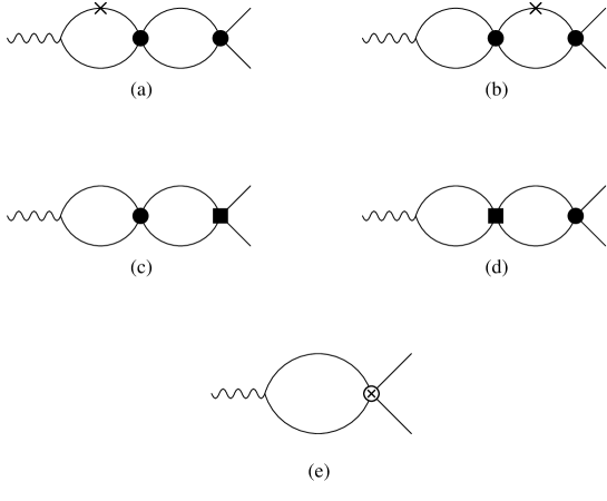
FIG. 14.: Diagrams which contribute to the two-loop anomalous dimension of the production current. The dot and box represent terms in the tree-level potential at order 1 ($V_{C}$), and $v^{2}$ ($V_{C}$, $V_{2}$, $V_{hf}$, $V_{LS}$, $V_{T}$) respectively. The $\otimes$ is an insertion of the order $v^{2}$ term proportional to $\alpha_{s}^{2}/m\left|\mathbf{k}\right|$ in the one-loop potential ($V_{\left|\mathbf{k}\right|}$). The $\times$ is an insertion of the $p^{4}/8m^{3}$ kinetic energy correction.

The contribution from the diagrams to the anomalous dimension will be called $\gamma_{a}$–$\gamma_{e}$, respectively, where

$$\mu_{\rm S}{dC\over d\mu_{\rm S}}=\nu{dC\over d\nu}=\gamma.$$ (62)

One finds that

$$\gamma_{a} = 0,$$ (63)

$$\gamma_{b} = -{1\over 64}V_{C}^{2},$$ (64)

$$\gamma_{c} = -{1\over 16}V_{C}\left(V_{2}+2V_{hf}\right)-{1\over 32}V_{C}^{2},$$ (65)

$$\gamma_{d} = -{1\over 32}V_{C}^{2},$$ (66)

$$\gamma_{e} = {\pi^{2}\over 2}V_{\left|\mathbf{k}\right|}$$ (67)

and the total anomalous dimension is

$$\gamma = \gamma_{a}+\gamma_{b}+\gamma_{c}+\gamma_{d}+\gamma_{e}=-{5V_{C}^{2}\over 64}-{V_{C}\left(V_{2}+2V_{hf}\right)\over 16}+{\pi^{2}V_{\left|\mathbf{k}\right|}\over 2}$$ (68)

which agrees with the known result for QCD at $\mu=m$, Eq. (53), when the coefficients Eq. (61) are used.

To complete the renormalization group analysis of the two-loop anomalous dimension, one needs the running values for $V_{C}$, $V_{hf}$ and $V_{\left|\mathbf{k}\right|}$, which will be presented elsewhere. Note, however, that our analysis disagrees with the results of [14], in which the running of these terms in the potential was neglected.

VI Conclusions

We have discussed a formulation of nonrelativistic QCD that can be used with a mass-independent subtraction scheme such as $\overline{\rm MS}$. The effective theory passes several non-trivial checks: (1) it has a consistent $v$ power counting expansion, (2) it correctly reproduces the running of the quark-antiquark potential at one loop, and (3) it correctly reproduces the two-loop running of the production current. The effective theory allows one to simultaneously treat the momentum regions of order $mv$ and $mv^{2}$.

In the way we have formulated the effective theory, all large logarithms have been summed at the scale $\nu=v$. At this point, one can integrate out the soft and modes, and at the same time switch from a theory of quarks and antiquarks to a theory of quarkonia, i.e. to an effective Lagrangian representing quarkonia interacting with background color fields, as first studied by Voloshin [30] and Leutwyler [31].

The methods described here should also be applicable to other nonrelativistic field theories, such as those describing nucleon-nucleon scattering at low energies [32].

- [1] For a review, see A.V. Manohar and M.B. Wise, Heavy Quark Physics, Cambridge University Press.
- [2] G.T. Bodwin, E. Braaten and G.P. Lepage, Phys. Rev. D51, 1125 (1995) hep-ph/9407339.
- [3] W.E. Caswell and G.P. Lepage, Phys. Lett. 167B, 437 (1986).
- [4] M. Beneke and V.A. Smirnov, Nucl. Phys. B522, 321 (1998) hep-ph/9711391.
- [5] P. Labelle, Phys. Rev. D58, 093013 (1998) hep-ph/9608491.
- [6] M. Luke and A.V. Manohar, Phys. Rev. D55, 4129 (1997) hep-ph/9610534.
- [7] A.V. Manohar, Phys. Rev. D56, 230 (1997) hep-ph/9701294.
- [8] B. Grinstein and I.Z. Rothstein, Phys. Rev. D57, 78 (1998) hep-ph/9703298.
- [9] M. Luke and M.J. Savage, Phys. Rev. D57, 413 (1998) hep-ph/9707313.
- [10] A.H. Hoang, Phys. Rev. D56, 5851 (1997) hep-ph/9704325.
- [11] A.H. Hoang, Phys. Rev. D56, 7276 (1997) hep-ph/9703404.
- [12] A. Czarnecki and K. Melnikov, Phys. Rev. lett. 80, 2531 (1998) hep-ph/9712222.
- [13] M. Beneke, A. Signer and V.A. Smirnov, Phys. Rev. lett. 80, 2535 (1998) hep-ph/9712302.
- [14] M. Beneke, A. Signer and V.A. Smirnov, Phys. Lett. B454, 137 (1999) hep-ph/9903260.
- [15] H.W. Griesshammer, Phys. Rev. D58, 094027 (1998) hep-ph/9712467.
- [16] A. Pineda and J. Soto, Nucl. Phys. Proc. Suppl. 64, 428 (1998) hep-ph/9707481.
- [17] A. Pineda and J. Soto, Phys. Lett. B420, 391 (1998) hep-ph/9711292.
- [18] A. Pineda and J. Soto, Phys. Rev. D58, 114011 (1998) hep-ph/9802365.
- [19] N. Brambilla, A. Pineda, J. Soto and A. Vairo, hep-ph/9907240.
- [20] T. Appelquist, M. Dine and I.J. Muzinich, Phys. Lett. 69B, 231 (1977).
- [21] T. Appelquist, M. Dine and I.J. Muzinich, Phys. Rev. D17, 2074 (1978).
- [22] W. Fischler, Nucl. Phys. B129, 157 (1977).
- [23] H. Georgi, Phys. Lett. B240, 447 (1990).
- [24] M. Luke and A.V. Manohar, Phys. Lett. B286, 348 (1992) hep-ph/9205228.
- [25] A. Pineda and J. Soto, Phys. Rev. D59, 016005 (1999) hep-ph/9805424.
- [26] S. Titard and F.J. Yndurain, Phys. Rev. D49, 6007 (1994) hep-ph/9310236.
- [27] S. Titard and F.J. Yndurain, Phys. Rev. D51, 6348 (1995) hep-ph/9403400.
- [28] B. Blok, J.G. Korner, D. Pirjol and J.C. Rojas, Nucl. Phys. B496, 358 (1997) hep-ph/9607233.
- [29] C. Bauer and A.V. Manohar, Phys. Rev. D57, 337 (1998) hep-ph/9708306.
- [30] M.B. Voloshin, Nucl. Phys. B154, 365 (1979).
- [31] H. Leutwyler, Phys. Lett. 98B, 447 (1981).
- [32] R. Seki, U. van Kolck and M.J. Savage, “Nuclear physics with effective field theory. Proceedings, Joint Caltech/INT Workshop, Pasadena, USA, February 26-27, 1998,” Singapore, Singapore: World Scientific (1998) 274 p.