Asymptotic scaling of the gluon
propagator on the lattice

Abstract

We pursue the study of the high energy behaviour of the gluon propagator on the lattice in the Landau gauge in the flavorless case ($n_{f}=0$). It was shown in a preceding paper that the gluon propagator did not reach three-loop asymptotic scaling at an energy scale as high as 5 GeV. Our present high statistics analysis includes also a simulation at $\beta=6.8$ ($a\simeq 0.03$ fm), which allows to reach $\mu\simeq 10$ GeV. Special care has been devoted to the finite lattice-spacing artifacts as well as to the finite volume effects, the latter being acute at $\beta=6.8$ where the volume is bounded by technical limits. Our main conclusion is a strong evidence that the gluon propagator has reached three-loop asymptotic scaling, at $\mu$ ranging from 5.6 GeV to 9.5 GeV. We buttress up this conclusion on several demanding criteria of asymptoticity, including scheme independence. Our fit in the 5.6 GeV to 9.5 GeV window yields $\Lambda^{\overline{{\rm MS}}}\ =\ 319\pm 14\ ^{+10}_{-20}$ MeV, in good agreement with our previous result, $\Lambda^{\overline{{\rm MS}}}\ =\ 295\pm 20$ MeV, obtained from the three gluon vertex, but it is significantly above the Schrödinger functional method estimate : $238\pm 19$ MeV. The latter difference is not understood. Confirming our previous paper, we show that a fourth loop is necessary to fit the whole ($2.8\div 9.5$) GeV energy window.

LPT Orsay/99-72

In previous works, we tackled the non-perturbative calculation of the QCD running coupling constant in two different ways: (i) by using the three gluon coupling [1, 2], and (ii) by matching the behaviour of the lattice regularized gluon propagator to the one predicted by perturbation theory [3]. The latter method was expected to take benefit of the very good statistical accuracy of the propagators and thus to yield a rather precise estimate of the strong coupling constant in its ultraviolet (UV) regime, i.e. of $\Lambda_{\rm QCD}$. Unluckily we could not fulfill this program for the unexpected reason that the gluon propagator has not yet reached the asymptotic scaling at scales of $\mathsf{2.5\div 5.0}$ GeV. This conclusion was supported by several different tests. In particular, the remainder of a strong scheme dependence when using one-, two- and three-loop formulae indicated the compelling need of higher orders in the perturbative expansion. Still we observed that the inclusion of third-loop corrections improved the asymptoticity (albeit not enough) over the two-loop results. We were naturally tempted to extend the analysis to higher energy scales where any perturbative expansion, with a fixed number of terms, should progressively improve. This is the basic motivation of the present paper.

Since we want to reach ever larger momenta on the lattice, we have to assure that the dominant lattice artifacts are under control. We must also ensure that the energy window, in which we could test scaling of the gluon propagator, is large enough. The reason is that at large scales, the coupling constant has a very mild logarithmic dependence. If the window is too narrow, the higher order terms might mimic the lower order ones, that we consider, and thus introduce a bias in $\Lambda_{\rm QCD}$. A very wide energy window has been explored in ref. [18] by using the Schrödinger functional technique. When using the methods based on Green functions [1, 2, 3], it is more difficult to vary the energy scales on several orders of magnitude. Moreover, one deals with more scales: the lattice spacing $a$, the linear lattice extension $L$, and the momenta of the gluons $p^{2}$. On the other hand, compared to the Schrödinger functional method, we believe that the Green functions have a simpler physical meaning and, being conceptually very different, represent a necessary test.

The requirement of larger momentum scales implies smaller lattice spacings if we are to keep the UV ${\cal O}(a^{2}p^{2})$ artifacts under control ($ap\ll 1$). Equivalently, we need to perform the simulations at larger $\beta$, which (for reasonable computing time) also means smaller volumes and potentially dangerous infrared (IR) finite volume artifacts. To prevent these problems, we need to ensure $Lp\gg 1$.

The question is whether we can find an ensemble of lattice results  fulfilling all requirements, i.e. that the lattice artifacts are small enough (${\cal O}(L^{-1})\ll p\ll{\cal O}(a^{-1})$), and that the energy window is large. This is a very demanding requirement because a small change in the coupling constant can induce a large uncertainty in $\Lambda_{\rm QCD}$. To avoid the statistical uncertainties in that respect, we work with $1.000$ independent gauge field configurations at every stage of this research . To keep the energy window large enough, we need to fit simultaneously the lattice data obtained at different lattice spacings. In other words, we must ensure that the small momentum lattice data with large $\beta$, and large momentum data with small (but reasonable) $\beta$, are compatible. In order to achieve that, and to reduce systematic uncertainties to the level of statistical ones, one evidently needs to control both IR and UV lattice artifacts for all the data. Therefore, a major part of this paper is devoted to these issues: the reduction of the UV and IR systematic uncertainties. The discretization errors are monitored by working at three values of the bare lattice coupling:

$$\beta\ =\ \left\{\hskip 19.91692pt6.0,\hskip 34.1433pt6.2,\hskip 39.83385pt6.8\hskip 19.91692pt\right\}\;.$$ (1)

A lattice spacing $a^{-1}=2.72(11)$ GeV has recently been measured at $\beta=6.2$ with a non-perturbatively improved action [16]. For a direct comparison with [1, 2, 3], in this paper we will keep $a^{-1}(\beta=6.2)=2.75$ GeV which is well within the error bars. Other lattices are calibrated relatively to this one, by using the lattice measurement of the string tension [15]. We take:

$$a^{-1}\ =\ \left\{\ 1.97\ {\rm GeV},\ 2.75\ {\rm GeV},\ 6.10\ {\rm GeV}\ \right\}\;,$$ (2)

at $\beta$ = 6.0, 6.2 and 6.8 respectively. Thus, our lattice spacings vary from $0.03$ fm to $0.10$ fm. The study at $\beta=6.8$ ($a\simeq 0.03$ fm) allows us to reach momenta up to $\sim 10$ GeV. The main study of the finite volume effects is performed at $\beta=6.0$, by repeating the calculation with the following lattice volumes:

$$V\ =\ \left\{\ 12^{4},\ 16^{4},\ 24^{4},\ 32^{4}\ \right\}\;.$$ (3)

From this study we deduced an efficient parametrization of the finite volume effects (18), which allows us to extrapolate our high momentum data to the $V\to\infty$ limit. An important cross check is provided by two volumes at $\beta=6.8$:

$$V\ =\ \left\{\ 16^{4},\ 24^{4}\ \right\}\;,$$ (4)

while for $\beta=6.2$, we work with the volume $V=24^{4}$ only.

An improved version of the method used in ref. [3] to cure lattice hypercubic effects, has been applied. The non-hypercubic finite spacing effects have been dealt with by comparing different values of $\beta$.

Curing the above-mentioned artifacts, we could keep most of our lattice points. We discarded those which exhibit large corrections.

In this paper, we will not deal with the small momentum behaviour of the gluon propagator. We postpone it to our forthcoming publications. This part has so far attracted a lot of attention in the literature [4]-[10] (for a review with a rather complete list of references, see ref. [11]), while, to our knowledge, the large momentum gluon propagator has not been studied in detail. Preliminary results of this paper were presented in ref. [12].

The remainder of this paper is organized as follows: In section 1 we outline the generalities of the method we use (previously described in ref. [3]), and introduce the main perturbation theory tools. In section 2, the lattice artifacts are discussed. Those related to hypercubic geometry are eliminated by improving the method presented in ref. [3]. A procedure allowing to treat empirically the finite-volume effects is described. In section 3 we perform a three-loop fit to the gluon propagator in the $\widetilde{\hbox{MOM}}$ scheme and apply the test of scheme independence, by considering a $(5.6\div 9.5)$ GeV window in which only the data at $\beta=6.8$ are used. Section 4 is devoted to the study of the whole window, ranging from 2.8 up to 9.5 GeV by combining all lattice data. We discuss our results in section 5 and conclude in section 6.

1 General description of the method

The Euclidean two point Green function in momentum space writes in the Landau gauge:

$$G_{\mu_{1}\mu_{2}}^{(2)\,a_{1}a_{2}}(p,-p)\ =\ \delta_{a_{1}a_{2}}\left(\delta_{\mu_{1}\mu_{2}}-\frac{p_{\mu_{1}}p_{\mu_{2}}}{p^{2}}\right)\ G^{(2)}(p^{2})\,,$$ (5)

where $a_{1},a_{2}$ are the color indices ranging from 1 to 8. The bare gluon propagator in the Landau gauge (see for instance ref. [3]), is such that

$$\lim_{\Lambda\to\infty}\frac{d\ln Z_{3}(\mu,\Lambda)}{d\ln\mu^{2}}\;\equiv\;\lim_{\Lambda\to\infty}\frac{d\ln[\mu^{2}G^{(2)}_{\rm bare}(\mu,\Lambda)]}{d\ln\mu^{2}}\,,$$ (6)

is independent of any regularization scheme. $Z_{3}(\mu,\Lambda)$ is the gluon renormalization constant in the MOM (or $\widetilde{\rm MOM}$) scheme at the point $p^{2}=\mu^{2}$, and $\Lambda$ is a generic notation for the UV cut-off ($a^{-1}$ or $(d-4)^{-1}$).

It is well known that the $\mu$ and the $\Lambda$ dependences of $Z_{3}(\mu,\Lambda)$ factorize when one drops all the terms vanishing as $\Lambda\to\infty$ (see ref. [13]), and we can write:

$$Z_{3}(\mu,\Lambda)=Z_{3}^{R}(\mu)Z_{3}^{b}(\Lambda)+{\cal O}(1/\Lambda)\;\;;$$ (7)

where the evolution of both, $Z_{3}^{R}(\mu)$ and $Z_{3}^{b}(\Lambda)$, is described by Callan-Symanzik equations

$$\left({d\over d\ln\mu^{2}}-\Gamma^{R}(\mu)\right)\ Z_{3}^{R}(\mu)\ =0\ ,$$

$$\left({d\over d\ln\Lambda^{2}}-\Gamma^{b}(\Lambda)\right)\ Z_{3}^{b}(\Lambda)\ =0\ .$$ (8)

From the QCD perturbation theory we know that

$$\frac{d\ln Z_{3}^{R}(\mu)}{d\ln\mu^{2}}=\Gamma^{R}(\mu)=-\left(\frac{\gamma_{0}}{4\pi}\alpha+\frac{\gamma_{1}}{(4\pi)^{2}}\alpha^{2}+\frac{\gamma_{2}}{(4\pi)^{3}}\alpha^{3}+O(\alpha^{4})\right)\,,$$ (9)

where it is understood that the coupling constant in a given scheme is a function of $\mu$ such that

$$\frac{\partial\alpha}{\partial\ln\mu}=\beta(\alpha)=-\frac{\beta_{0}}{2\pi}\alpha^{2}-\frac{\beta_{1}}{(2\pi)^{2}}\alpha^{3}-\frac{\beta_{2}}{(4\pi)^{3}}\alpha^{4}+O(\alpha^{5})$$ (10)

with

$$\beta_{0}=11,\quad\beta_{1}=51,\quad\gamma_{0}=\frac{13}{2}\,,$$ (11)

in the flavorless case ($n_{f}=0$), while $\gamma_{1},\gamma_{2}$ and $\beta_{2}$ are scheme dependent. To be specific, in the flavorless $\widetilde{\hbox{MOM}}$ scheme:

$$\beta_{2}\simeq 4824.,\quad\gamma_{1}=\frac{29}{8},\quad\gamma_{2}\simeq 960\,.$$ (12)

Lattice calculations provide us with the bare propagator but in a finite volume which, besides the UV cut-off ($\Lambda\sim 1/a$), introduces an additional length dimension, $L$ (the physical volume being $L^{4}$). As we shall see, finite volume effects, as well as hypercubic artifacts, should be eliminated first in order to have access to the renormalization constant in eq. (6), $Z_{3}(\mu,1/a)$.

Equations formally analogous to (9) and (10) can be obtained from the second line of eq. (8), with the substitutions of $1/a$ for $\Lambda$ and of the lattice bare coupling constant, $\alpha^{b}=3/(2\pi\beta)$, for the renormalized one. Unhappily the anomalous dimension coefficients, $\gamma_{1}^{b},\gamma_{2}^{b}$, have not been determined to our knowledge, presumably due to the difficulty of the task. Any perturbative calculation of $Z_{3}^{b}(1/a)$ appears thus to be limited to one loop,

$${d\ln Z_{3}^{b}(1/a)\over d\alpha^{b}(1/a)}\ ={\gamma_{0}^{b}\over\beta_{0}}{1\over\alpha^{b}(1/a)}$$ (13)

for which it can easily be proven that $\gamma_{0}^{b}=-\gamma_{0}$.

Our general “strategy”, as explained in ref. [3], will be to integrate simultaneously eqs. (9,10), up to three loops in a given scheme. The solutions depend on the initial values $Z^{R}_{3}(\mu_{0})$ and $\alpha(\mu_{0})$. They are related to the lattice results, $Z_{3}(\mu,1/a)$, through eq. (7). When we restrict our computation to the lattice data at $\beta=6.8$, $Z^{b}_{3}(1/a)$ is just an overall irrelevant multiplicative constant. With our three values of $\beta$, two ratios of three ($Z^{b}_{3}(6.8)/Z^{b}_{3}(6.2)$, $Z^{b}_{3}(6.8)/Z^{b}_{3}(6.0)$, $Z^{b}_{3}(6.2)/Z^{b}_{3}(6.0)$) are necessary for appropriate matching of all our lattice data. These ratios will be fitted and compared to one-loop predictions in section 4.

Finally, the knowledge of $\alpha(\mu_{0})$ in a given scheme allows the determination of $\Lambda_{QCD}$ in this scheme, and hence of $\Lambda_{\rm QCD}^{\overline{\rm MS}}$.

2 Lattice artifacts

We refer to ref. [1] for technical details concerning the lattice setup in our simulations, the calculation of the Green functions, their Fourier transform, the checks of the $\delta_{a_{1},a_{2}}$ color dependence of the propagators, and the set of momenta considered for the different lattices studied. Since the release of ref. [1], we increased the statistical quality of our data, and further explored various lattice volumes and various values of $\beta$. As mentioned in the introduction, of special interest for this study are the results of our simulation performed at $\beta=6.8$, at two volumes: $16^{4}$ and $24^{4}$. The high statistical accuracy of our data made a detailed study of systematic uncertainties possible and mandatory.

2.1 Hypercubic artifacts and other $(a^{2}p^{2})$ effects

We start with the discretization errors. In a finite hypercubic volume the momenta are the discrete sets of vectors

$$p_{\mu}\ =\ \frac{2\pi}{L}\ n_{\mu}\;,$$ (14)

where the components of $n_{\mu}$ are integers and $L$ is the lattice size. The propagators have been averaged as usual, over the hypercubic isometry group $H_{4}$. The momenta corresponding to different orbits of $H_{4}$, but belonging to the same orbit of the continuum isometry group $SO(4)$ (e.g. $n_{\mu}=(2,0,0,0)$, and $n_{\mu}=(1,1,1,1)$), have been analyzed according to an improved version of the method proposed in ref. [3].

Let us briefly recall the elements of that method. The main idea is based on the fact that, on the lattice, an invariant scalar form factor, like $G^{(2)}(p^{2})$, is indeed a function of 4 invariants $p^{[n]}\equiv\sum_{\mu}p_{\mu}^{n}$, $n=2,4,6,8$. We will neglect the invariants with degree higher than 4 since, in any case, they vanish at least as $\sim a^{4}$. Thus, we parametrize and expand the lattice two-point scalar form factor as a function of the two remaining invariants which, on dimensional grounds, appear as $p^{2}$ and $a^{2}p^{[4]}$:

$$G_{\rm lat}^{(2)}(p^{2},a^{2}p^{[4]};L,a)=G_{\rm lat}^{(2)}(p^{2},0;L,a)\ +\ \left.{\partial G\over\partial(a^{2}p^{[4]})}\right|_{a^{2}p^{[4]}=0}a^{2}p^{[4]}\ .$$ (15)

$\left.{\partial G/\partial(a^{2}p^{[4]})}\right|_{a^{2}p^{[4]}=0}$ is a symbolic notation for the lattice hypercubic slope. This equation summarizes our method to reduce hypercubic artifacts and contains all the assumptions on which the method relies. We make the hypothesis that the lattice propagator for the discrete momenta belonging to different $H_{4}$-orbits takes values according to a certain continuous functional behaviour. When several orbits exist for one $p^{2}$, to the extent that a linear approximation is licit, the hypercubic slope can be extracted and the extrapolation to $a^{2}p^{[4]}=0$, by using eq. (15), can be made. We have checked that the linear approximation (15) is indeed good enough. This is what has been done in ref. [3]. Now we elaborate further on this method in order to improve its accuracy and extend its applicability.

A simple dimensional argument leads to: $\left.{\partial G/(a^{2}\partial p^{[4]})}\right|_{a^{2}p^{[4]}=0}\propto 1/p^{4}$, as $L\to\infty$, suggesting the fitting form $b/p^{4}$, where $b$ is a constant . At this point, from the study of the lattice hypercubic slope for different values of $\beta$, we extracted the values of term $b/p^{4}$ and examined the behaviour of the remainder. We find that the logarithm of $\left(-b+p^{4}\left.{\partial G/(a^{2}\partial p^{[4]})}\right|_{a^{2}p^{[4]}=0}\right)$ is well described by a linear function of $Lp$. This leads us to:

$$\left.{\partial G\over\partial(a^{2}p^{[4]})}\right|_{a^{2}p^{[4]}=0}=\ {b\over p^{4}}\ \biggl{(}1+c\ \exp(-d\ Lp)\biggr{)}\ .$$ (16)

By fitting our data to the above form and by keeping $\chi^{2}/d.o.f.\simeq 1$ (see Fig.1a), we obtained the following set of parameters:

lj $\beta$	$b$	$c$	$d$
lj 6.0	0.117(9)	1.1(1.5)	0.15(8)
lj 6.2	0.109(2)	1.9(1.2)	0.18(3)
lj 6.8	0.100(5)	0.6(8)	0.13(5)

Table 1: The values of the parameters $b$, $c$, $d$, as obtained by fitting our data to eq.(16).

The values for $c$ and $d$ in Tab. 1 are presented to show the order of magnitude. Their errors, estimated by using the jackknife method, are misleading since the parameters are strongly correlated. A refined statistical study is not necessary for our purpose, since we follow the jackknife analysis cluster by cluster to the end.

On the other hand it is rewarding that the errors on $b$ in (1) are small, which is essential for an accurate infinite volume limit. It is also encouraging that $b$ varies only slowly with $a$, which justifies our neglecting higher order terms, ${\cal O}(a^{4}\ p^{[6]})$ etc., and it clearly confirms that we do control the lattice hypercubic artifacts. We can now take advantage of the good fit obtained with eq. (16) and compute the lattice hypercubic slope in cases where only one orbit exists (for instance, when $n^{2}=5$, we only have $n_{\mu}=(2,1,0,0)$ and its $H_{4}$ orbit).

(a)
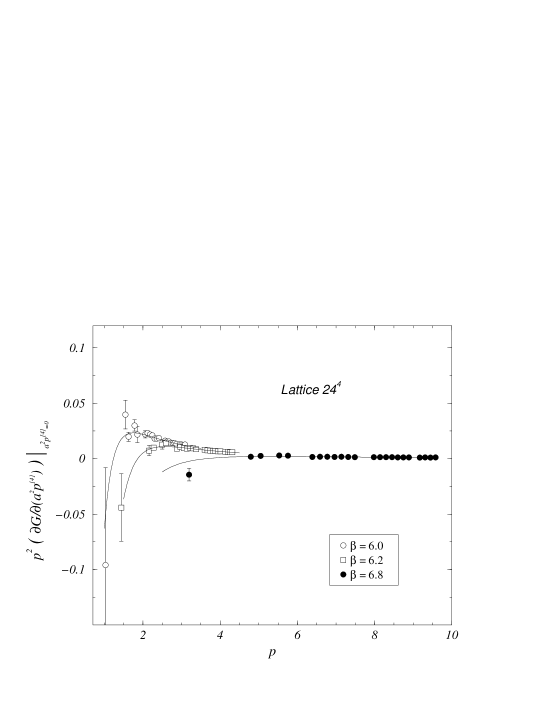
(b)

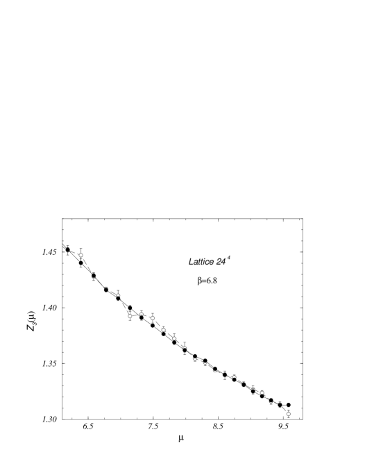
Figure 1: Plot (a) shows $p^{2}\left.{\partial G\over a^{2}\partial p^{[4]}}\right|_{a^{2}p^{[4]}=0}$, as a function of the scale $p$ evaluated on $24^{4}$ lattices at $\beta=6.0,6.2,6.8$. Plot (b) compares the “hypercubic-free propagator” defined from eqs. (15,16) (black circles) and the propagator computed by direct extrapolation to $a^{2}p^{[4]}=0$ (white circles), plotted as a function of the momentum.

To summarize, by using eq. (16), we extrapolate $G_{\rm lat}^{(2)}(p^{2},a^{2}p^{[4]};L,a)$ to what we will call the hypercubic-free propagator, $G_{\rm lat}^{(2)}(p^{2},0;L,a)$. In ref. [3], we discussed the improvement brought in by our previous ($a^{2}p^{[4]}=0$)-extrapolation approach with respect to other methods to reduce hypercubic artifacts. The use of eq. (16) allows even better accuracy on slopes: not only does it allow an extrapolation to $a^{2}p^{[4]}=0$ when only one orbit exists but it also helps to reduce the uncertainty by taking benefit of the neighboring values of $n^{2}$ when the error is locally too large. The outcome of this improvement is depicted in Fig. 1b, where the resulting curve joining the points obtained by using eq. (16) is much smoother than the one obtained by separate extrapolation  for each $n^{2}$.

It is important to add that not all ${\cal O}(a^{2})$ artifacts are eliminated: for instance, the lattice artifacts $\propto a^{2}\ p^{2}$, which do not break $SO(4)$ invariance, are still present. One way to deal with this problem is to compare the data at different values of $\beta$. One can also study the stability of the results when the maximum value of $p^{2}$ used in the fits is varied. We have checked this stability in the fits presented below.

2.2 Finite volume effects

After removing hypercubic artifacts, we are left with the hypercubic-free propagator. The dependence on the length scale, $L$, as we previously mentioned, is apparent from Fig. 2. The elimination of this additional length scale should be done in order to compute the renormalization constant for the Landau gauge gluon propagator,

$$Z_{3}(\mu,1/a)\ =\ \lim_{L\to\infty}\bigl{(}p^{2}G_{\rm lat}^{(2)}(p^{2},0;L,a)\bigr{)}_{p^{2}=\mu^{2}}\ .$$ (17)

In doing so, we will not attempt a theoretical understanding of the expected finite volume dependence of the bare propagator. We will be content if we obtain a reliable empirical parametrization for the dependence on the lattice volume of $G_{\rm lat}^{(2)}(p^{2},0;L,a)$ which will allow us to take the required limit (17). For dimensional reasons, we will take it as a function of $Lp$ and $a/L$. We note that the difference amongst the data at fixed $\beta$ and various volumes gets bigger as we move towards lower $p^{2}$. This is illustrated in Fig. 2 where we plot $p^{2}G_{\rm lat}^{(2)}(p^{2},0;L,a)$. We tried several ansätze for this parametrization function and finally found that

$$G_{\rm lat}^{(2)}(p^{2},0;L,a)\ =\ G_{\rm lat}^{(2)}(p^{2},0;\infty,a)\ \left(1+v_{1}\left({a\over L}\right)^{4}+v_{2}\exp(-v_{3}Lp)\right)\ ,$$ (18)

with

$$v_{1}=450(40),\;\;\;\;v_{2}=0.44(16),\;\;\;v_{3}=0.177(25),$$ (19)

gives the best fit to the behaviour on $L$ of hypercubic-free propagators evaluated on $12^{4}$, $16^{4}$, $24^{4}$, $32^{4}$ lattices in the energy window  ($1.5\div 3.0)$ GeV at $\beta=6.0$. This parametrization is not efficient at lower energies, as it can be seen in Fig. 2b.

(a)		(b)

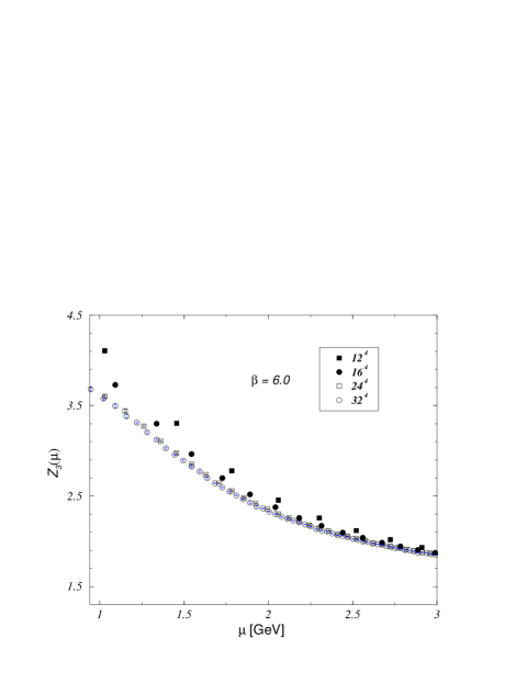
Figure 2: Plot (a) contains the hypercubic-free propagators evaluated on $12^{4}$ (black squares), $16^{4}$ (black circles), $24^{4}$ (white circles), $32^{4}$ (white squares) lattices at $\beta=6.0$. The same data extrapolated to $L\to\infty$ according to the parametrization given by eqs. (18,19) are plotted in (b) .

Once the parametrization function from propagators evaluated at $\beta=6.0$ is established, it can be applied to our results at $16^{4}$ and $24^{4}$ lattices at $\beta=6.8$. The agreement after extrapolation shown by the curves resulting from the extrapolation in Fig. 3 is a crucial test for the validity of such a parametrization for the finite volume effects.

(a)		(b)

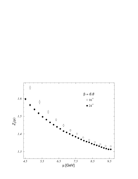
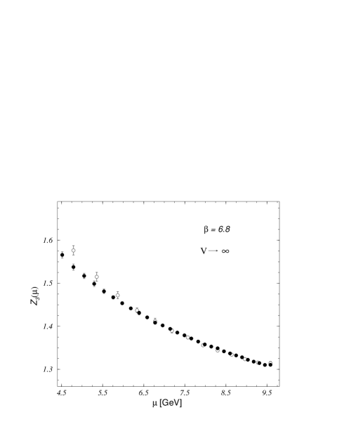
Figure 3: This figure is analogous to Fig. 2 for $\beta=6.8$. Black (white) circles correspond to $24^{4}$ ($16^{4}$) lattices.

Thus, eqs. (17-19) lead to a non-perturbative evaluation of the renormalization constant, $Z_{3}(\mu,1/a)$, which is precisely the quantity we want to compare to the predictions of perturbative QCD.

3 Fitting in the $\widetilde{\rm MOM}$ scheme at high energies

In this section we perform the matching of the perturbative predictions for $\widetilde{\rm MOM}$ renormalization constant to our lattice result at high energies. We follow the method outlined in section 1 and refer the reader to ref. [3] for more details.

We consider the coupled differential equations (9,10) in the $\widetilde{\rm MOM}$ scheme, where the coefficients $\gamma_{1}$, $\gamma_{2}$, $\beta_{2}$ are those given in eq. (12). We fit our data at $\beta=6.8$ for $Z_{3}(\mu,1/a)$, with a solution of these coupled equations in the energy window $(5.6\div 9.5)$ GeV. The result of this fit is

$$Z_{3}(9.5\ {\rm GeV})=1.3107(9),\quad\alpha_{\widetilde{\rm MOM}}(9.5\ {\rm GeV})=0.190(3),\quad\chi^{2}/{d.o.f.}=0.29\,.$$ (20)

The $\chi^{2}/d.o.f$ is significantly smaller than $1$ which may be a sign of some correlation between the points at different values of the energy $\mu$.

As explained in [3], $\Lambda^{\overline{\rm MS}}$ can be estimated from the above quantities (20), by using the perturbative expressions to two- and three-loop accuracy. We obtain:

$$\Lambda_{(3\rm{loop})}^{\overline{\rm MS}}\ \simeq\ 0.346\;\Lambda_{(3\rm{loop})}^{\widetilde{\rm MOM}}\ =\ 319\pm 14\ {\rm MeV},\quad$$ (21)

(22)

$$\Lambda_{(2\rm{loop})}^{\overline{\rm MS}}\ \simeq\ 0.346\;\Lambda_{(2\rm{loop})}^{\widetilde{\rm MOM}}\ \simeq\ 375\ {\rm MeV},$$ (23)

where the error is only statistical at this stage. The existence of a good fit (see Fig. 4) by itself is not a sufficient proof of asymptoticity: next-to-three-loop corrections could be mimicked by a simple rescaling of $\Lambda_{\rm QCD}$ in the considered energy range [3]. This is why we developed a consistent method to test asymptoticity by exploring the scheme dependence within the domain of so-called “good schemes”: one investigates the dispersion of the result for $\Lambda^{\overline{\rm MS}}$ when we vary the schemes , by varying $\gamma_{1}$ and $\gamma_{2}$, in all the possible ways such that the successive terms in the perturbative series (9,10) are at most as large as the preceding ones . In ref. [3], we found that this dispersion is of $\sim 35$ MeV, for $\Lambda^{\overline{\rm MS}}$ fixed from the fit of the gluon propagator at $\sim 4$ GeV to the three-loop perturbative expression. In the present study, when fixing $\Lambda^{\overline{\rm MS}}$ at around $9.5$ GeV, this dispersion (in the same domain of schemes) is of $\sim 10$ MeV only.

Note that the difference in eq. (23) between two and three loops, although smaller than at $4$ GeV, is still sizable indicating the necessity to include the third loop term.

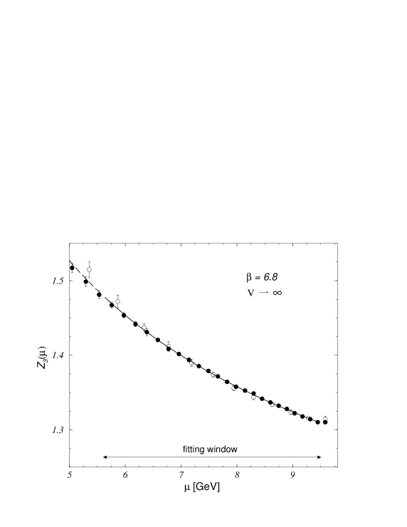
Figure 4: The plot shows (full line) the best fit to $Z_{3}(\mu,1/a)$ with the three-loop formula together with the lattice results at $\beta=6.8$ after extrapolation to $L\to\infty$ from both $16^{4}$ and $24^{4}$ lattice volumes, for $5.6\ {\rm GeV}<\mu<9.5{\rm GeV}$. The fit is continued outside the energy window as a dashed line.

4 Global description and asymptotic pattern

Our analysis at high energy in the previous section seems to establish that a signal of three-loop perturbative scaling is found in the energy window $(5.6\div 9.5)$ GeV. By including the data obtained at $\beta=6.0$ and $\beta=6.2$, one can make the energy window larger: $2.8$ GeV$\lesssim\mu\lesssim 9.5$ GeV (the choice for the lower limit will be discussed below). However, as already mentioned in the end of Sec. 1, any global fit involves two additional parameters, the ratios $Z_{3}^{b}(6.0)/Z_{3}^{b}(6.8)$ and $Z_{3}^{b}(6.2)/Z_{3}^{b}(6.8)$. Moreover, we do not expect a three-loop perturbative behaviour to work in the whole energy window. In ref. [3], we showed that the propagator was not asymptotic to three-loops at $\sim 4$ GeV. The difference between $\Lambda_{(3\rm{loop})}^{\overline{\rm MS}}$ in eq. (23) and $\sim 350$ MeV as found in ref. [3], confirms that statement. Thus, at least the fourth loop correction is necessary for the global fit. Unfortunately, such a perturbative result is not available in the ${\widetilde{\rm MOM}}$ scheme.

With these fives free parameters, a global fit turns out to be unstable. A global study of our lattice data would nevertheless enable a direct test of consistency for the the whole information we extract from gluon propagator. For that reason we adopt the following strategy. First, we take the value of $\Lambda^{\overline{\rm MS}}_{\rm(3loop)}$ given in eq. (23), to be the asymptotic one, i.e. we assume the gluon propagator to reach asymptotia at three-loop for the energy window studied in the previous section. Then we fix the fourth loop correction to the three-loop perturbative expression, by fitting the data obtained in our simulations at $\beta=6.0$ and $\beta=6.2$, corresponding to the energy range $(2.8\div 4.3)$ GeV. Once, the fourth loop correction is known, we will verify the asymptoticity of the gluon propagator in the entire energy window ($2.8\div 9.5$) GeV.

The four-loop information about the gluon propagator in ${\widetilde{\rm MOM}}$-scheme is encoded in the coefficients $\gamma_{3}^{\widetilde{\rm MOM}}$ and $\beta_{3}^{\widetilde{\rm MOM}}$. These two coefficients are not independent but related through the expression [14, 3]

$$\frac{\gamma_{3}^{\widetilde{\rm{MOM}}}}{(4\pi)^{4}}+\frac{\beta_{3}^{\widetilde{\rm{MOM}}}}{(4\pi)^{4}}\frac{\gamma_{0}}{\beta_{0}}=\frac{\gamma_{3}}{(4\pi)^{4}}+\frac{\beta_{3}}{(4\pi)^{4}}\frac{\gamma_{0}}{\beta_{0}}\ ,$$ (24)

which is valid for any renormalization scheme in which $\gamma_{1}=\gamma_{1}^{\widetilde{\rm{MOM}}}$, $\gamma_{2}=\gamma_{2}^{\widetilde{\rm{MOM}}}$ and $\beta_{2}=\beta_{2}^{\widetilde{\rm{MOM}}}$, listed in eq. (12). Thus, there is only one free parameter to be fitted. For simplicity, we choose among the set of schemes satisfying  (24), the one with $\beta_{3}=0$, $\widehat{\gamma_{3}}$ being that free parameter. For such a renormalization scheme,

$$Z^{R}(\mu)\ =\ Z^{(3)}(\mu)\ \exp\left(\frac{1}{3(4\pi)^{3}}\frac{\widehat{\gamma}_{3}}{\beta_{0}}\ (\widehat{\alpha}^{3}(\mu)-\alpha^{3}_{0}\ )\ \right)$$ (25)

(a)
(b)

Figure 5: One-, two-, three- and four-loop perturbative curves obtained from our best fits of $\alpha_{\widetilde{\rm{MOM}}}(9.5\rm{GeV})$ and $\widehat{\gamma}_{3}$ are presented in plot (a). Notice that all these curves are computed with $\Lambda^{\widetilde{\rm MOM}}\ =\ 319\pm 14\ {\rm MeV}$. The points correspond to the lattice evaluations at $\beta=6.0$, $6.2$ divided by our best fits of the ratios of $Z^{b}_{3}$ referred to $\beta=6.8$ ($Z^{b}_{3}$ is taken to be $1$ at $\beta=6.8$). Plot (b) shows the same perturbative curves and the lattice data at $\beta=6.8$.

is, up to higher irrelevant orders, the solution to the four-loop coupled equations analogous to (9) and (10), where $Z^{(3)}(\mu)$ is the solution of the three-loop problem, with $\alpha_{0}$ being the initial strong coupling constant at $\mu_{0}$ for both, three- and four-loops. The results of the fit in the energy window $(2.8\div 4.3)$ GeV read (see Fig. 5)

$$\frac{Z^{b}_{3}(a(6.0))}{Z^{b}_{3}(a(6.8))}\ =\ 0.995(3)\ ,\quad\;\frac{Z^{b}_{3}(a(6.2))}{Z^{b}_{3}(a(6.8))}\ =\ 1.012(2)\ ,$$

$$\widehat{\gamma}_{3}\ =\ (2.2\pm 1.6)\cdot 10^{4}\quad\quad\left(\chi^{2}/{d.o.f.}=1.17\right)\,;$$ (26)

where the errors on the ratios of $Z^{b}_{3}$’s do not take into account the uncertainty coming from the errors on the lattice spacing ratios. This uncertainty does not exceed one percent. When the lower limit of the energy window takes values below $2.8$ GeV, the $\chi^{2}/d.o.f.$ rapidly increases, which indicates the end of the four-loop matching. This is illustrated in Fig. 6a. The upper limit is fixed by $ap\leq\pi/2$. We note also that the fitted values of the ratios (26) are very close to $1.0$, and somewhat larger than the results obtained by using the one-loop lattice perturbation theory .

The estimated $\widehat{\gamma}_{3}$, is not as large as it might look:

$${\widehat{\gamma}_{3}\ \alpha/4\pi\over\gamma_{2}}\simeq 0.6\,,\quad{\rm and}\quad{\widehat{\gamma}_{3}\ \alpha^{3}/(4\pi)^{3}\over\gamma_{0}}\sim 0.05\,$$ (27)

at $\mu=4.0$ GeV. The large error for $\widehat{\gamma_{3}}$ quoted in eq. (26) is not surprising because the determination of $\widehat{\gamma}_{3}$ strongly depends on $\alpha_{\widetilde{\rm MOM}}(9.5\ {\rm GeV})$. In other words, a very small uncertainty on $\alpha_{\widetilde{\rm MOM}}$ reflects in large error for $\widehat{\gamma}_{3}$, in our energy window $(2.8\div 4.3)$ GeV. Thus the computation of the value for $\widehat{\gamma_{3}}$ from perturbation theory would considerably reduce the systematic uncertainty of $\alpha_{\widetilde{\rm MOM}}(9.5\ {\rm GeV})$, and hence of $\Lambda^{\overline{\rm MS}}$.

(a)
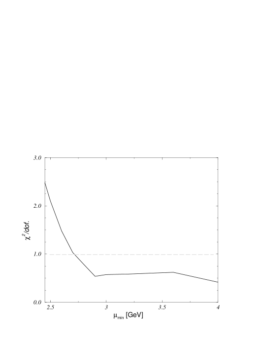
(b)

Figure 6: Plot(a): the $\chi^{2}/{\rm d.o.f.}$ for the global fit obtained after the estimation of the four-loop contribution as a function of the lower limit for the energy window. Plot (b): the global fit of all the lattice results with the four-loop corrected perturbative formula (the full line curve on Fig. 5) from eq. (25).

At this point, we can check the consistency by performing a global fit over the entire window $2.8\ {\rm GeV}\leq\mu\leq 9.5$ GeV, with the values of $\widehat{\gamma}_{3}$ and of the ratios $Z^{b}_{3}$ taken from (26). The result of such a fit is depicted in Fig. 6. The global estimate of $\Lambda^{\overline{\rm MS}}$ does not modify the one we obtained at large energies ($5.6\ {\rm GeV}\leq\mu\leq 9.5$ GeV) given in eq. (23), whereas the global $\chi^{2}/{d.o.f.}$ is $0.79$.

Finally, we should assess the systematic uncertainty introduced by the assumption of the three-loop asymptoticity (i.e. $\widehat{\gamma_{3}}=0$), for $5.6\ \rm{GeV}\ \leq\ \mu\ \leq\ 9.5\ \rm{GeV}$. The simplest estimate of the non-asymptoticity errors consists in monitoring the value of $\Lambda^{\overline{\rm MS}}$, while varying the coefficient $\widehat{\gamma_{3}}\neq 0$. $|\widehat{\gamma_{3}}|$ is reasonably bounded by $4\pi\gamma^{\widetilde{\rm MOM}}_{2}/\alpha(\mu)$ over the whole window. From the previous works [3, 18] and from the present study we see that the non-asymptoticity has a tendency to provoke overestimates of $\Lambda^{\overline{\rm MS}}$ (the effective $\Lambda^{\overline{\rm MS}}_{\rm(3loop)}$ decreases as the matching is performed at higher energies). This observation is sufficient to exclude the negative values of $\widehat{\gamma_{3}}$. Then, by varying $0\leq\widehat{\gamma_{3}}\leq 4\pi\gamma^{\widetilde{\rm MOM}}_{2}/\alpha(5.6\rm{GeV})\sim 42000$ we obtain the uncertainty in $\Lambda^{\overline{\rm MS}}$ of $\sim 20$ MeV. Thus, the Landau gauge gluon propagator analysis results in

$$\Lambda^{\overline{\rm MS}}=319\pm 14^{+10}_{-20}\ ,$$ (28)

where the upper limit for the systematic uncertainty comes from the dispersion we observed by exploring the domain of three-loop good schemes, around ${\widetilde{\rm MOM}}$, over the ($\gamma_{1},\gamma_{2}$)-plane. It is important to note that the uncertainty on the value of $\Lambda^{\overline{\rm MS}}$ would be considerably reduced if the value $\gamma^{\widetilde{\rm MOM}}_{3}$ was known. Not only the $-20$ MeV would be reduced, but also the dispersion over the set of good schemes to four loops would be fairly restrained.

Reciprocally, if $\Lambda^{\overline{\rm MS}}$ was known accurately from any other source, we could use our data to fit $\widehat{\gamma}^{3}$ rather accurately. For example taking $\Lambda^{\overline{\rm MS}}$ strictly equal to the central value in eq. (28), would give

$$\left.\frac{\gamma_{3}^{\widetilde{\rm{MOM}}}}{(4\pi)^{4}}+\frac{\beta_{3}^{\widetilde{\rm{MOM}}}}{(4\pi)^{4}}\frac{\gamma_{0}}{\beta_{0}}\quad\right|_{\Lambda^{\overline{\rm MS}}=319\,{\rm MeV}}=\ 0.88\pm 0.04.$$ (29)

where we have used eq. (24). But let us repeat, the fitted value for $\widehat{\gamma}^{3}$ varies quickly when $\Lambda^{\overline{\rm MS}}$ is varied within the error bars, which explains the large error in (26) or equivalently:

$$\frac{\gamma_{3}^{\widetilde{\rm{MOM}}}}{(4\pi)^{4}}+\frac{\beta_{3}^{\widetilde{\rm{MOM}}}}{(4\pi)^{4}}\frac{\gamma_{0}}{\beta_{0}}=0.9\pm 0.6.$$ (30)

5 Discussion

The estimate of $\Lambda^{\overline{{\rm MS}}}$ is significantly higher than the one obtained with the Schrödinger functional [18], $\Lambda^{\overline{{\rm MS}}}=238\pm 19$ MeV. Zero flavour NRQCD results [19], although not directly expressed in terms of $\Lambda^{\overline{{\rm MS}}}$, seem to agree with the result from Schrödinger functional. Estimates from string tension cover a large range of values: $244(8)$ MeV [15], $293(18)^{+25}_{-63}$ MeV [20]. On the other hand, the value recently obtained directly from the triple gluon vertex, $\Lambda^{\overline{{\rm MS}}}=295\pm 20$ MeV in [1], and the less recent $340(50)$ MeV [2], along with the one obtained in this paper, favor the larger values of $\Lambda^{\overline{{\rm MS}}}$. The discrepancy is of the order of three sigma. Method based on Schrödinger functional and the one based on Green functions are quite different so that a direct comparison is not easy. Could it be that the reason for this discrepancy is simply that we did not reach a enough large energy ? In other words, could it be that the difference between $\Lambda^{\overline{{\rm MS}}}=238\pm 19$ MeV and the result (28) were simply due to the fact that next to third order terms, which are not used in the fit leading to (28), do mimic a larger $\Lambda^{\overline{{\rm MS}}}$ ? To investigate this question we use a simple check: had we assumed the result for $\Lambda^{\overline{{\rm MS}}}$ in ref. [18] to be the right asymptotic one, we would have obtained

$$\left.\frac{\gamma_{3}^{\widetilde{\rm{MOM}}}}{(4\pi)^{4}}+\frac{\beta_{3}^{\widetilde{\rm{MOM}}}}{(4\pi)^{4}}\frac{\gamma_{0}}{\beta_{0}}\quad\right|_{\Lambda^{\overline{\rm MS}}=238\,{\rm MeV}}=\ 8.42\pm 0.08\ ,$$ (31)

over the same energy window used for (29), $(2.8\div 9.5)$ GeV, the $\chi^{2}/{\rm d.o.f.}$ being $0.89$. The Schrödinger functional result applied to our data would then imply that the Landau gauge gluon propagator is not asymptotic at three-loops at the energy scale of $9$ GeV. The four-loop contribution in this case would be much bigger than the three-loop one (about four times). This seems rather unlikely! We therefore conclude that the value $\Lambda^{\overline{{\rm MS}}}$ obtained by using the Schrödinger functional technique is difficult to accommodate with the gluon propagator data by using the three-loop expression. There may be some unknown systematic effect explaining this discrepancy.

Let us finally make a comment about the convergence of the gluon propagator. The direct connection between the renormalization constant in the ${\widetilde{\rm MOM}}$-scheme and the gluon propagator makes the gluon momentum the natural scale in this scheme. The scales in the ${\widetilde{\rm MOM}}$-scheme are significantly larger than the corresponding ones in the ${\overline{\rm MS}}$ scheme, typically by a factor 1/0.346 (see eq. (23). The Landau pole in the ${\widetilde{\rm MOM}}$ scheme is around $1$ GeV. As the perturbative regime of the propagator is expected to settle in when $\log(\mu/\Lambda_{{\widetilde{\rm MOM}}})$ is large enough, it is then not too surprising that high perturbative orders are important around $\sim 3$ GeV and higher energies are needed to reach a three-loop perturbative scaling.

6 Conclusions

The main goal of the present work was to go deeper into the study of the asymptoticity of the Landau gauge gluon propagator. The matching of its non-perturbative evaluation from lattice with perturbative predictions, gives us an estimate of the strong coupling constant and hence of $\Lambda^{\rm{QCD}}$ [3].

We have carefully examined the lattice spacing effects, particularly the hypercubic artifacts, and the finite volume ones. We find a close linearity in $a^{2}p^{[4]}$ of the gluon propagator, with the slope given by eq. (16) which removes efficiently the hypercubic artifacts. The finite volume effects, in the region of large momenta, are parametrized by the relation (18).

After having subtracted the lattice artifacts, we found that the four-loop contribution is negligible above $\mathsf{\sim 5.}$ GeV, but becomes important below this energy, confirming the conclusion of ref. [3]. In its turn the four-loop perturbative scaling fails below $\mathsf{2.8}$ GeV: the Landau gauge gluon propagator reaches very slowly the asymptotia.

We therefore have fitted with a three-loop formula over the energy window $5.6\ {\rm GeV}\ \leq\ \mu\ \leq\ 9.5\ {\rm GeV}$. The rather good fit leads to $\Lambda_{(3\rm{loop})}^{\overline{{\rm MS}}}\ =\ 319\pm 14$ MeV. A fitted four-loop formula has been used to extend the fit over the larger energy window ($2.8\div 9.5$) GeV. We have obtained a consistent description of all our lattice data.

Our final result is

$$\Lambda^{\overline{{\rm MS}}}\ =\ 319\pm 14^{+10}_{-20}\;\;\;\frac{a^{-1}(6.2)}{2.75{\rm GeV}}\;\;\;{\rm MeV}\ \ ,$$ (32)

with the errors discussed in detail in Sec. 4. Although a combination of theoretical results is always delicate, we may try to combine this result with the one obtained from the study of the three gluon vertex [1], $\Lambda^{\overline{{\rm MS}}}=295\pm 20$ MeV. This results in an overall flavorless estimate from the gluon Green functions : $275\ \rm{MeV}\leq\Lambda^{\overline{{\rm MS}}}\leq 343\ \rm{MeV}$ .

References

- [1] Ph. Boucaud, J.P. Leroy, J. Micheli, O. Pène and C. Roiesnel, JHEP10 (1998) 017, [hep-ph/9810322 ].
-
[2]
B. Alles, D. Henty, H. Panagopoulos, C. Parrinello, C. Pittori, D.G. Richards, Nucl. Phys. B502 (1997) 325;
C. Parrinello et al, Nucl. Phys. Proc. Suppl. 63 (1998) 245, [hep-lat/9710053 ];
B. Alles, D. Henty, H. Panagopoulos, C. Parrinello, C. Pittori, IFUP-TH-23-96, [hep-lat/9605033 ]. - [3] D. Becirevic, Ph. Boucaud, J.P. Leroy, J. Micheli, O. Pène, J. Rodríguez–Quintero, C. Roiesnel, LPT Orsay-99/16, [hep-ph/9903364] (to appear in Phys.Rev. D).
- [4] C. Bernard, C. Parrinello and A. Soni, Phys. Rev. D49 (1994) 1585.
-
[5]
P. Marenzoni, G. Martinelli and N. Stella, Nucl. Phys. B455 (1995) 339, [hep-lat/9410011];
P. Marenzoni, G. Martinelli, N. Stella and M. Testa Phys. Lett. B318 (1993) 511. - [6] D.B. Leinweber, J.I. Skullerud, A.G. Williams and C. Parrinello, Nucl. Phys. B544, (1999) 669.
- [7] H. Nakajima and S. Furui, Nucl. Phys. Proc. Suppl. 73 (1999) 635 [hep-lat/9809081].
- [8] A. Nakamura and S. Sakai, Prog. Theor. Phys. Suppl. 131 (1998) 585.
-
[9]
A. Cucchieri,
Phys. Rev. D60 (1999) 034508, [hep-lat/9902023];
A. Cucchieri, T. Mendes, [hep-lat/9902024]. - [10] J.P. Ma, [hep-lat/9903009].
-
[11]
J.E. Mandula, Phys. Rept. 315 (1999) 273, [hep-lat/9903009];
P. Weisz, Nucl. Phys. Proc. Suppl. 47 (1996) 866, [hep-lat/9511017].. - [12] D. Becirevic, P. Boucaud, J.P. Leroy, J. Micheli, O. Pene, J. Rodriguez-Quintero and C. Roiesnel, [hep-lat/9908056].
- [13] G. Grunberg, Phys. Rev. D29 (1984) 2315.
- [14] Ph. Boucaud , J.P. Leroy, J. Micheli, O. Pène and C. Roiesnel, JHEP 12 (1998) 004, [hep-ph/9810437].
- [15] G.S. Bali and K. Schilling, Phys. Rev. D47 (1993) 661.
- [16] D. Becirevic et al., [hep-lat/9809129].
- [17] T.A. Springer, Lecture Notes in Mathematics 585, Springer-verlag (1977).
-
[18]
S. Capitani, M. Lüscher, R. Sommer,
H. Wittig, Nucl. Phys. B544 (1999) 669, [hep-lat/9810063].;
M. Lüscher, in “Probing the Standard Model of particle interactions”, Les Houches, Session LXVIII, (North Holland,), pp. 229, [hep-lat/9802029];
M. Lüscher, R. Sommer, P. Weisz, U. Wolf, Nucl. Phys. B413(1994) 481, [hep-lat/9309005 ]. - [19] C.T.H. Davies et al., Phys. Lett. B345 (1995) 42, [hep-ph/9408328 ], Phys. Rev. D56 (1997) 2755, [hep-lat/9703010].
- [20] G.S.Bali, In Protvino 1993, “Problems on high energy physics and field theory” (147-163), Protvino 1993, [hep-lat/9311009].