Penguin diagrams in the $\Delta I=1/2$ rule and $\epsilon^{\prime}/\epsilon$ with $\sigma$ models

Abstract

We study the correlation between ${\epsilon^{\prime}/\epsilon}$ and $\Delta I=1/2$ rule in the framework of non-linear $\sigma$ model including scalar mesons. Using this model we estimate the chiral corrections by resumming to all orders in Chiral Perturbation Theory, the contribution of a class of diagrams within the factorization approximation. With these matrix elements and changing the scalar meson mass, we find that there is correlation between ${\epsilon^{\prime}/\epsilon}$ and $\Delta I=1/2$ amplitude. However, it is difficult to explain both ${\epsilon^{\prime}/\epsilon}$ and $\Delta I=1/2$ amplitude simultaneously. In order to be compatible with ${\epsilon^{\prime}/\epsilon}$, typically, about half of $\Delta I=1/2$ amplitude can be explained at most. Our result suggests there may be substantial non-factorizable contribution to CP conserving $K\rightarrow\pi\pi$ amplitudes.

I Introduction

According to recent measurements of direct CP violation in $K\rightarrow\pi\pi$ decays, ${\epsilon^{\prime}/\epsilon}$ is $O(10^{-3})$ [1, 2]. Theoretical prediction ranges around $10^{-4}\sim 10^{-3}$. It strongly depends on the hadronic matrix elements of QCD [3] and EW penguin operators [4, 5, 6].

An interesting possibility is suggested as an explanation for large ${\epsilon^{\prime}/\epsilon}=O(10^{-3})$ in the standard model [7]. The authors argue that the mechanism which enhances $\Delta I=1/2$ amplitude may also enhance ${\epsilon^{\prime}/\epsilon}$ and it naturally leads to the measured values. The enhancement comes from the Feynman diagram which includes the scalar $\sigma$ meson as intermediate state. The mechanism was found in the framework of linear $\sigma$ model [8, 9]. Though qualitative picture of the linear $\sigma$ model may be correct, for quantitative analysis, some improvement can be made. In the linear $\sigma$ model employed in Ref.[9], $\sigma$ meson mass can be written in terms of the physical quantities $F_{K},F_{\pi},M_{K}$ and $M_{\pi}$ and its mass is predicted to be about $900$ MeV. SU(3) breaking ratio ${m_{u}/m_{s}}$ is also determined by the same input and numerically it is around ${1/30}$. The enhancement factor of a QCD penguin operator is written as ${F_{K}/(3F_{\pi}-2F_{K})}=({M_{n}\sigma}^{2}-{M_{\pi}}^{2})/({M_{\sigma}}^{2}-{M_{K}}^{2})\cdot({F_{K}}^{2}/{F_{\pi}}^{2})\simeq 2.$ These relations and numbers are specific predictions of the linear $\sigma$ model. Because the dynamical property of the linear $\sigma$ model is not same as that of QCD, these relations and numbers may be taken as semi-quantitative [7].

In this paper, we study the matrix elements of the QCD and EW penguins with the non-linear $\sigma$ model including scalar mesons. The model is built with chiral symmetry as a guide. It is more general than the linear $\sigma$ model and less dependent on dynamical assumption. The cost is that it has more parameters. They can be determined with the experimental measured quantities, i.e., decay width, mass spectrum, etc. Still $\sigma$ meson mass is left as a free parameter because the spectroscopy of $\sigma$ meson $f_{0}(400-1200)$ allows wide range for the mass. (See Refs. [10, 11, 12, 13, 14, 15] for scalar meson mass spectroscopy.) We study how QCD and EW penguin matrix elements depend on the mass of $\sigma$ meson.

Here we write a few words on the difference between our approach and the conventional treatment of the resonances in Chiral Perturbation Theory (CHPT). CHPT is a systematic treatment, in the sense of the small momentum expansion, and describes low energy processes involved pions and kaons well. However higher order terms in CHPT are of great importance if threshold of the $\sigma$ meson is near to kaon mass. Thus it is very interesting to explore non-linear $\sigma$ model with scalar resonances in kaon decays. Correspondence between non-linear $\sigma$ model with resonances and CHPT was well discussed in Refs.[16, 17] at order of $p^{4}$ and their results indicate that the resonance contributions dominate the low energy coupling constants in the strong part of $p^{4}$ chiral lagrangian. In our approach, we compute the full contribution of the $\sigma$ meson to the factorizable part of QCD and EW penguins using non-linear $\sigma$ model with scalar resonances, so that a certain class of higher order terms of $p^{n}(n>4)$ in momentum expansion are included. We show how these higher order terms contribute to observable in kaon decays.

As a phenomenological application, we compute ${\epsilon^{\prime}/\epsilon}$ and $\Delta I=1/2$ amplitude in isospin limit. We use the Wilson coefficients for four-fermi interaction at $\mu=0.8\sim 1.2$ GeV in the next to leading log (NLL) approximation [18, 19, 20]. The four-fermi operator is factorized into products of color singlet currents (or densities) and they are identified with those of the $\sigma$ model [21]. The density$\times$density type operators are enhanced for small strange quark mass by a factor of $(1/m_{s})^{2}$. Therefore numerical values for the strange quark mass are important. As for the strange quark mass, we choose the range which is suggested by QCD sum rule [22] and lattice simulations [23]. We also study the correlation between ${\epsilon^{\prime}/\epsilon}$ and $\Delta I=1/2$ amplitude. This is done by varying the $\sigma$ mass, strange quark mass $m_{s}$, and factorization scale $\mu$. By studying the dependence of ${\epsilon^{\prime}/\epsilon}$ and $\Delta I=1/2$ amplitude on the $\sigma$ meson mass, we search for the range of the mass which may reproduce both $\displaystyle{{\epsilon^{\prime}/\epsilon}}$ and $\Delta I=1/2$ amplitude.

The paper organized as follows: In section II, we summarize the outline of the computation ${\epsilon^{\prime}/\epsilon}$ and $\Delta I=1/2$ amplitude. In section III, we derive the matrix elements of penguin operators. In section IV, numerical results of ${\epsilon^{\prime}/\epsilon}$ and $\Delta I=1/2$ are summarized. In section V, we discuss the implication of our results. Some useful formulae are collected in appendix.

II $\Delta I=1/2$ rule and ${\epsilon^{\prime}/\epsilon}$ in the standard Model

In this section, we summarize our notations and show outline of computation of ${\epsilon^{\prime}/\epsilon}$ and $\Delta I=1/2$ amplitude. Some details of definitions of isospin amplitudes can be found in appendix A. We start with the effective hamiltonian for $\Delta S=1$ non-leptonic decays [18],

$$H_{eff}={G_{F}\over\sqrt{2}}V_{ud}V_{us}^{*}\sum_{i=1}^{10}\{z_{i}+\tau y_{i}\}Q_{i}+h.c,$$ (1)

where $\tau=-(V_{td}V_{ts}^{*})/(V_{ud}V_{us}^{*})$. The isospin amplitudes of $K\rightarrow\pi\pi$ are defined as $\langle I|H_{eff}|K^{0}\rangle=ia_{I}\exp{i\delta_{I}},\quad\langle I|H_{eff}|\bar{K^{0}}\rangle=-i{a_{I}}^{*}\exp{i\delta_{I}}$. $\epsilon^{\prime}$ is expressed in terms of $a_{0}$ and $a_{2}$.

$$\epsilon^{\prime}={1\over\sqrt{2}}{Rea_{2}\over Rea_{0}}({Ima_{2}\over Rea_{2}}-{Ima_{0}\over Rea_{0}})\exp\{i(\delta_{2}-\delta_{0}+{\pi\over 2})\}.$$ (2)

In the factorization approximation, $a_{I}$ s are written as,

$$Rea_{I}={G_{F}\over\sqrt{2}}ReV_{ud}V_{us}^{*}$$ (3)

$$\times\sum_{i=1}^{5}\left[(z_{2i-1}+{z_{2i}\over{N_{c}}})\langle I|Q_{2i-1}|K^{0}\rangle+(z_{2i}+{z_{2i-1}\over{N_{c}}})\langle I|Q_{2i}|K^{0}\rangle\right]\frac{1}{i},$$ (4)

$$Ima_{I}=-{G_{F}\over\sqrt{2}}ImV_{td}V_{ts}^{*}$$ (5)

$$\times\sum_{i=1}^{5}\left[(y_{2i-1}+{y_{2i}\over{N_{c}}})\langle I|Q_{2i-1}|K^{0}\rangle+(y_{2i}+{y_{2i-1}\over{N_{c}}})\langle I|Q_{2i}|K^{0}\rangle\right]\frac{1}{i},$$ (6)

where the matrix elements $\langle I|Q_{i}|K^{0}\rangle$ is defined in large $N_{c}$ limit. As we discuss in detail in the next section, we compute the hadronic matrix element in large $N_{c}$ limit, i.e., we factorize the four-fermi operators into products of color singlet currents (densities). The currents (densities) are identified with those of the chiral lagrangian. The factorization scale is chosen at $0.8$ $-$ $1.2$ GeV, i.e., below charm quark mass $m_{c}$. In the factorization approximation, this choice is mandatory because above $m_{c}$, real part of the Wilson coefficient of QCD penguin operators is zero and it is born below $m_{c}$ due to the incomplete cancellation of GIM mechanism. About Wilson coefficients, we use NLL approximation [18, 19, 20] and compute them at the factorization scale. Combining the matrix elements with the Wilson coefficients, $a_{I}$ s are given as,

$$Rea_{0}={G_{F}\over\sqrt{6}}\lambda\frac{X}{i}\left[2z_{2}+3z_{4}-z_{1}+3z_{6}{Y_{6}\over X}\right],$$ (7)

$$Rea_{2}={G_{F}\over\sqrt{3}}\lambda\frac{X}{i}\left[z_{1}+z_{2}\right],$$ (8)

$$Ima_{0}={-\sqrt{3}G_{F}\over\sqrt{2}}\frac{X}{i}{(A\lambda^{2})}^{2}\lambda\eta\left[y_{4}+\frac{y_{7}-y_{9}+y_{10}}{2}+y_{6}\frac{Y_{6}}{X}+{2\over 3}y_{8}\frac{\tilde{Y}_{8}-\frac{3}{4}Y_{6}}{X}\right],$$ (9)

$$Ima_{2}={-\sqrt{3}G_{F}\over 2}\frac{X}{i}{(A\lambda^{2})}^{2}\lambda\eta\left[{-y_{7}+y_{9}+y_{10}}+\frac{2}{3}y_{8}\frac{\tilde{Y}_{8}}{X}\right],$$ (10)

where matrix elements are denoted by $X$, $Y_{6}$, and ${\tilde{Y}}_{8}$. $X$ is the matrix element of current$\times$current type operators, $Y_{6}$ corresponds to the matrix element of a density$\times$density QCD penguin operator, ${\tilde{Y}}_{8}$ is the matrix element of EW penguin operator. Their derivation and precise definition will be given in the next section and are summarized in Table I and II.

III Non-linear $\sigma$ model including scalar mesons and the matrix elements of QCD and EW Penguin operators

The non-linear $\sigma$ model with higher resonances are studied in [16, 17]. In $K\rightarrow\pi\pi$ decays, in large $N_{c}$ limit, scalar meson may contribute to the matrix elements of density$\times$density type four-fermi operators ($Q_{6}$, $Q_{8}$). For current$\times$current type four-fermi interactions, the amplitude is proportional to the form factor of semi-leptonic decay, i.e., ${f_{+}}({M_{K}}^{2}-{M_{\pi}}^{2})+{f_{-}}M_{\pi}^{2}$. Because the form factors $f_{\pm}(q^{2})$ near soft-pion limit ($q^{2}={M_{\pi}}^{2}$) are important, vector mesons contribution to the form factors is small and their effect can be safely neglected. Therefore we include only scalar mesons in chiral lagrangian,

$${\cal L} = {f^{2}\over 4}Tr\partial U\partial U^{\dagger}+B~{}Tr{\cal M}(U+U^{\dagger})+{g_{1}\over 4}Tr\partial U\partial U^{\dagger}{\xi S\xi^{\dagger}}$$ (11)

$$+ g_{2}~{}Tr{\cal M}(\xi S\xi+\xi^{\dagger}S\xi^{\dagger})+Tr(DSDS-{M_{\sigma}}^{2}S^{2}),$$ (12)

where ${\cal M}=diag(m_{u},m_{d},m_{s})$, $U=\exp\left(i2\pi/f\right)=\xi^{2}$ and $S$ is a scalar nonet field,

$$S=\frac{1}{2}\left(\begin{array}[]{ccc}\sigma+\delta^{0}&\sqrt{2}\delta^{0}&\sqrt{2}\kappa^{+}\\ \sqrt{2}\delta^{0}&\sigma-\delta^{0}&\sqrt{2}\kappa^{0}\\ \sqrt{2}{\kappa^{-}}&\sqrt{2}\bar{\kappa^{0}}&\sqrt{2}\delta_{ss}\end{array}\right).$$ (16)

$DS$ is covariant derivative and is defined by,

$$D_{\mu}S = \partial_{\mu}S+i[\alpha_{//\mu},S],$$ (17)

$$\alpha_{//\mu} = {\xi^{\dagger}\partial_{\mu}\xi+\xi\partial_{\mu}\xi^{\dagger}\over 2i}={[\pi,\partial_{\mu}\pi]\over 2if^{2}}+\ldots$$ (18)

In the lagrangian, the scalar mesons couple to pions through two terms denoted by $g_{1}$ and $g_{2}$. One is a coupling in SU(3) limit and the other is a coupling with SU(3) breaking. The mass splitting term for the scalar nonets and isospin breaking effect are neglected. By shifting the scalar meson fields from their vacuum expectation value,

$$S\rightarrow S+<S>,~{}~{}~{}<S>={g_{2}\over{M_{\sigma}}^{2}}{\cal M},$$ (19)

we obtain the mass formulae and decay constants [16]. They are given in the appendix B. The parameters in the chiral lagrangian can be written in terms of physical quantity $F_{K},F_{\pi},M_{K},M_{\pi}$ and quark masses $m_{u}(=m_{d})$ and $m_{s}$.

$$B={2\over m_{s}(1-\Delta)}\left[{(\Delta+1)M_{\pi}^{2}F_{\pi}^{2}\over 8\Delta}-{\Delta M_{K}^{2}F_{K}^{2}\over 2(1+\Delta)}\right],$$ (20)

$${g_{2}^{2}\over{M_{\sigma}}^{2}}={2\over m_{s}^{2}(1-\Delta)}\left[-{F_{\pi}^{2}M_{\pi}^{2}\over 4\Delta}+{F_{K}^{2}M_{K}^{2}\over 2(1+\Delta)}\right],$$ (21)

$${g_{1}g_{2}\over{M_{\sigma}}^{2}}={2(F_{K}^{2}-F_{\pi}^{2})\over m_{s}(1-\Delta)},$$ (22)

where $\Delta={m_{u}/m_{s}}$. For computation of the weak matrix elements, we need strong interaction vertices. They can be found in appendix C.

In our calculation using the lagrangian Eq.(12), a certain class of the higher order terms in the CHPT are summed up due to the effect of the scalar resonance exchange. These are very important in the process $K\rightarrow\pi\pi$ if the $\sigma$ meson mass is light as kaon mass, $M_{\sigma}\sim M_{K}$. Though systematic treatment of momentum expansion in the CHPT is lost, a class of the higher order terms in the CHPT are automatically summed up using lagrangian of Eq.(12).

Now we turn to the matrix element of QCD and EW penguins. The explicit derivation is given for two density$\times$density type operators $Q_{6}$ and $Q_{8}$. Their definitions are,

$$\displaystyle Q_{6} = -8\sum_{q=u,d,s}({\bar{s}_{L}}q_{R})({\bar{q}_{R}}d_{L}),$$ (23)

$$Q_{8} = -12\sum_{q=u,d,s}({\bar{s}_{L}}q_{R})e_{q}({\bar{q}_{R}}d_{L})={\tilde{Q}}_{8}-\frac{1}{2}Q_{6},$$ (24)

$${\tilde{Q}}_{8} = -8({\bar{s}_{L}}u_{R})({\bar{u}_{R}}d_{L}),$$ (25)

where the subsidiary operator ${\tilde{Q}}_{8}$ is introduced. These operators can be written in terms of meson fields by identifying quark bilinear as corresponding density,

$$\bar{q}_{R}^{j}q_{L}^{i}=-BU_{ij}-g_{2}\left(~{}\xi(S+\langle S\rangle)\xi~{}\right)_{ij}.$$ (26)

After some algebra, we express $Q_{6}$ in terms of the meson fields,

$$Q_{6} = -8\left[~{}~{}\frac{i}{\sqrt{2}}{g_{2}^{2}(m_{s}-m_{u})\over{M_{\sigma}}^{2}}\left(2B+{g_{2}^{2}(m_{s}+m_{u})\over{M_{\sigma}}^{2}}\right){K^{0}\over F_{K}}\right.$$ (27)

$$- \left.{i\over 24\sqrt{2}}{g_{2}^{2}(m_{s}-m_{u})\over{M_{\sigma}}^{2}}\left(2B+{g_{2}^{2}(m_{s}+m_{u})\over{M_{\sigma}}^{2}}\right){{K^{0}{\pi^{0}}^{2}}\over{F_{K}F_{\pi}^{2}}}\right.$$ (28)

$$- \left.{ig_{2}\over 2\sqrt{2}}\left\{\left(2B+g_{2}^{2}{(m_{s}+m_{u})\over{M_{\sigma}}^{2}}\right){\pi^{0}\kappa\over F_{\pi}}+\left(2B+{g_{2}^{2}2m_{u}\over{M_{\sigma}}^{2}}\right){\sigma K^{0}\over F_{K}}\right\}~{}~{}\right].$$ (29)

There are four diagrams which may contribute to $K^{0}\rightarrow\pi^{0}\pi^{0}$ amplitude $Y_{6}$. (See Feynman diagrams in Fig.3 - Fig.5) They are classified as follows.
1) The diagram in which $K^{0}$ decays into $K^{0}\pi^{0}\pi^{0}$ through the strong vertex and subsequently $K^{0}$ vanishes into vacuum through the $Q_{6}$ ( $T_{tadpole}$).
2) The diagram in which $K^{0}$ directly decays into $2\pi^{0}$ ($T_{direct}$).
3) The diagram in which $K^{0}$ is converted into $\sigma$ and subsequently $\sigma$ decays into $2\pi^{0}$ ($T_{\sigma\mbox{-}pole}$).
4) The diagram in which K decays into $\kappa,\pi^{0}$ through strong vertex and $\kappa$ is converted into $\pi^{0}$ ($T_{\kappa\mbox{-}pole}$).
The sum of the contribution is denoted by $Y_{6}$ and it can be simplified as,

$$Y_{6} = {i\sqrt{2}\over F_{K}F_{\pi}^{2}}\left[~{}-{g_{1}g_{2}\over{M_{\sigma}}^{2}}\left\{\bar{B}_{0}{M_{K}^{2}\over 1-\delta_{\pi}^{2}}+\bar{B}{M_{K}^{2}-2M_{\pi}^{2}\over 1-\delta_{k}^{2}}\right\}\right.$$ (32)

$$+{g_{2}^{2}\over{M_{\sigma}}^{2}}\left\{{4\bar{B}_{0}\over 1-\delta_{\pi}^{2}}\left(m_{s}+m_{u}-{(m_{s}-m_{u})M_{K}^{2}\over 2{M_{\sigma}}^{2}}\right)-{8\bar{B}m_{u}\over 1-\delta_{k}^{2}}-(m_{s}-m_{u})\left(2\bar{B}_{0}+\bar{B}(1+{1\over R^{2}})\right)\right\}$$

$$-\left.{g_{1}g_{2}^{3}\bar{B}(m_{s}-m_{u})^{2}\over 2F_{K}^{2}{M_{\sigma}}^{4}}+{g_{2}^{4}(m_{s}-m_{u})^{2}\over{M_{\sigma}}^{4}}~{}\right],$$

where $R={F_{K}/F_{\pi}}$ and $\delta_{K(\pi)}={M_{K(\pi)}/M_{\sigma}}$. We also introduce the auxiliary quantities,

$$\bar{B}=B+{g_{2}^{2}(m_{s}+m_{u})\over 2{M_{\sigma}}^{2}},~{}~{}~{}~{}~{}\bar{B}_{0}=B+{g_{2}^{2}m_{u}\over{M_{\sigma}}^{2}}.$$ (33)

They can be written in terms of physical quantities,

$$\bar{B}={M_{K}^{2}F_{K}^{2}\over 2m_{s}(1+\Delta)},~{}~{}~{}~{}~{}~{}~{}~{}\bar{B}_{0}={M_{\pi}^{2}F_{\pi}^{2}\over 4m_{s}\Delta}.$$ (34)

The matrix element of EW penguin operator $Q_{8}$ is straightforward. Technically we split $Q_{6}$ from $Q_{8}$ so that we do not have to repeat the calculation of $Q_{6}$. The rest is called ${\tilde{Q}}_{8}$ and given by,

$${\tilde{Q}}_{8}=\left[ig_{2}\bar{B}_{0}\frac{\pi^{-}\kappa^{+}}{F_{\pi}}-i\frac{g_{2}\bar{B}_{0}(\bar{B}_{0}+\bar{B})}{\sqrt{2}}\frac{K^{0}\pi^{+}\pi^{-}}{F_{K}F_{\pi}^{2}}\right]+\cdots.$$ (35)

In $K^{0}\rightarrow\pi^{+}\pi^{-}$ amplitude, there are two contributions to the hadron matrix element of $\widetilde{Q}_{8}$, i.e., (a) $\kappa$-pole contribution and (b) direct contribution. The sum is called ${\tilde{Y}}_{8}$ and is given by,

$${\tilde{Y}}_{8} = -i\frac{3}{\sqrt{2}F_{K}F_{\pi}^{2}}\frac{\bar{B}_{0}}{{M_{\sigma}}^{2}-M_{\pi}^{2}}\left[g_{1}g_{2}M_{K}^{2}-2g_{2}^{2}\left\{(m_{s}+3\bar{m})-(m_{s}-\bar{m})\frac{M_{K}^{2}-M_{\pi}^{2}}{{M_{\sigma}}^{2}}\right\}\right]$$ (37)

$$+i6\sqrt{2}\frac{1}{F_{K}F_{\pi}^{2}}\bar{B}_{0}\left(\bar{B}+\bar{B}_{0}\right).$$

Keeping leading terms of $1/M_{\sigma}$ the matrix elements $Y_{6},\tilde{Y}_{8}$ reduce to the well known results $Y_{6}^{0},\tilde{Y}_{8}^{0}$ [24], which correspond to those in the leading order of momentum expansion and in large $N_{c}$ limit.

$$Y_{6}^{0}=-4\sqrt{2}i\left(F_{K}-F_{\pi}\right)\left(\frac{M_{K}^{2}}{m_{s}+m_{u}}\right)^{2},~{}~{}~{}~{}~{}\tilde{Y}_{8}^{0}=3\sqrt{2}iF_{\pi}\left(\frac{M_{K}^{2}}{m_{s}+m_{u}}\right)^{2}.$$ (38)

This approximation is valid only when $M_{K}\ll M_{\sigma}$. In the next section we will show how the values of the matrix elements of the density$\times$density operators are different from $Y_{6}^{0},\tilde{Y}_{8}^{0}$ numerically.

The matrix elements of the other current$\times$current operators $Q_{i}(i\neq 6,8)$ are also shown in Table I and II, and are expressed by a single amplitude X:

$$X=i\sqrt{2}f({M_{K}}^{2}-{M_{\pi}}^{2}).$$ (39)

IV Numerical Results

In this section, we first estimate the hadronic parameters $B_{6,8}$ corresponding to the matrix element $Q_{6}$ and $Q_{8}$ in the factorization approximation. We compare our results with those from the linear $\sigma$ model. As an application, we also compute $\epsilon^{\prime}/\epsilon$ and $Rea_{0},Rea_{2}$. This is done in isospin limit.

The conventional bag-factors $B_{6}^{1/2}$, $B_{8}^{3/2}$, which people often refer, is defined by the following equation in our notation,

$$B_{6}^{1/2}=\frac{Y_{6}}{Y_{6}^{0}},~{}~{}~{}~{}~{}B_{8}^{3/2}=\frac{2\tilde{Y_{8}}-X}{2\tilde{Y_{8}^{0}}-X}.$$ (40)

As explained in section III, using $M_{\pi}$, $M_{K}$, $F_{\pi}$, $F_{K}$ as inputs our model can be described by three free parameters in the lagrangian $M_{\sigma}$, $m_{s}$, $\Delta=m_{u}/m_{s}$ and another parameter $\mu$ in the matching process which is the factorization scale.

We find that our model predicts that the factorizable part of $B_{6}^{1/2}$ ranges around $1.6\sim 3.0$ depending on the $\sigma$ meson mass $M_{\sigma}$. The quark mass dependence is not significant. On the other hand, $B_{8}^{3/2}$ ranges around $0.7\sim 1.1$ depending on $\Delta$. We varied $\Delta$ in the range of $1/20-1/30$ and smaller $\Delta$ gives larger value of $B_{8}^{3/2}$. $M_{\sigma}$ dependence is negligible for $B_{8}^{3/2}$. The numerical value is given in Table III.

Let us now compare our results with those from linear $\sigma$ model [9]. The factorizable bag-factors are given by the following equations.

$$B_{6}^{1/2} = \frac{F_{K}}{3F_{\pi}-2F_{K}}\sim 2,$$ (41)

$$B_{8}^{3/2} \simeq \frac{F_{K}}{F_{\pi}}\sim 1.2,$$ (42)

Because there are only four parameters in the linear $\sigma$ model lagrangian, after using $M_{\pi,K},F_{\pi,K}$ there are no free parameters left, so that the model predicts $\Delta=1/30$ and $M_{\sigma}\sim 0.9$ GeV.

From Table III we find that $B_{8}^{3/2}$ from our model with $\Delta=1/30$ and that from the linear $\sigma$ model are consistent. It can be seen that the factorizable part of $B_{6}^{1/2}$ for $M_{\sigma}=0.9$ GeV is around 1.5, which is smaller than the linear $\sigma$ model result.

Next we apply our result to $\epsilon^{\prime}/\epsilon$ and $Rea_{0},Rea_{2}$. For numerical computation of ${\epsilon^{\prime}/\epsilon}$, we use the experimental values for $Rea_{I}$.

We have calculated the next to leading order Wilson coefficients in NDR scheme. we could reproduce the numerical values tabulated in Ref. [18] to a good extent. We chose the following values for the computation, $m_{t}$ = 165.00 GeV, $m_{W}$ = 80.20 GeV, $m_{b}$ = 4.40 GeV, $m_{c}$ = 1.30 GeV, $1/\alpha_{QED}$ = 129.0, $sin^{2}(\theta_{W})$ = 0.230, $\Lambda_{QCD}^{(5)}$ = 0.226 GeV, $\Lambda_{QCD}^{(4)}$ = 0.325 GeV, $\alpha^{\overline{MS}}(m_{Z})^{(5)}$ = 0.11799. We list the Wilson coefficients $z_{i},y_{i}$ at scales $\mu$ = 1.2, 1.0, 0.8 GeV in Table IV. In this calculation, we used the anomalous dimensions at the NLO by Buras et al.

As was explained in section II, in the leading order in large $N_{c}$ expansion, $Rea_{I},Ima_{I}$ are obtained by multiplying Wilson coefficients $z_{i}(\mu),y_{i}(\mu)$ with the matrix elements of $Q_{1}(\mu),\cdots,Q_{10}(\mu)$ in our model, where $\mu$ is the factorization scale which is assumed to be 0.8 $-$ 1.2 GeV.

Here we should remark one point about the quark mass. In large $N_{c}$ limit, we approximate the matrix elements with $Q_{6}(\mu)$ operator by the product of matrix elements with scalar quark operator at scale $\mu$. Using PCAC relation, we then convert them to $F_{K}M_{K}^{2}/m_{s}(\mu)$. Here, the scale of the strange quark mass should be the same scale $\mu$. Therefore, when we substitute the mass parameter $m_{s}$ in our final result, we should run the quark mass to the factorization scale $\mu$=0.8,1.0,1.2 GeV. For example, $m_{s}$(2GeV)= 80 $-$ 120 MeV corresponds to $m_{s}$(0.8GeV)=136 $-$ 204 MeV.

Figure 1 shows the dependence of $\eta$ from our model on the scalar resonance mass $M_{\sigma}$. Here, we take $m_{s}^{\overline{MS}}$(2GeV)=80,120,180 MeV, which cover the recent QCD calculations [22, 23], and the scale $\mu$ is chosen to be 0.8 GeV. Upper and lower lines correspond to the maximum and minimum values of $\epsilon^{\prime}/\epsilon$, respectively. We find that when $M_{\sigma}$ is larger than $0.8$ GeV in order for $\eta$ to lie within 0.27-0.52, which is favored by other measurements of CKM parameters, $m_{s}^{\overline{MS}}$(2GeV) should take rather small value 0.09 $-$ 0.12 GeV. These values are consistent with recent lattice QCD calculations [23] but smaller compared with QCD sum rule results [22]. On the other hand, as $M_{\sigma}$ becomes smaller the $Q_{6}$ amplitude gets enhanced, in order for $\eta$ to lie within 0.27-0.52, larger value of $m_{s}^{\overline{MS}}$(2GeV) is preferred.

Finally, in Figure 2, we show the correlation of $\displaystyle{a_{0}/a_{0}^{\rm exp}}$ and $\displaystyle{\epsilon^{\prime}/\epsilon}$ by changing the scalar meson mass from 0.6 GeV to 1 GeV. We take three different values of $m_{s}^{\overline{\rm MS}}$(2GeV), which are 80, 100 and 120 MeV. We take three values for the factorization scale $\mu$, which are 0.8, 1.0 and 1.2 GeV. We used the experimental values of $Rea_{I}$ for the numerical analysis of ${\epsilon^{\prime}/\epsilon}$. CP violation parameter is chosen to be 0.3 in the figure. The shaded region is the experimental data from KTeV and NA48 for $\displaystyle{\epsilon^{\prime}/\epsilon}$ at 2-$\sigma$ confidence level.

We find that $\displaystyle{\epsilon^{\prime}/\epsilon}$ can be easily explained in our model by a suitable choice of the parameters. Typical value of $M_{\sigma}$, and $m_{s}^{\overline{\rm MS}}$(2GeV) is around 0.8 GeV and around 80 MeV respectively almost independent of the factorization scale $\mu$. On the other hand, $Rea_{0}$ in our model are smaller than experiment. We find that it is quite sensitive to the factorization scale $\mu$, and as $\mu$ gets smaller, $Rea_{0}$ becomes larger towards the experimental value. For $\mu$=0.8 GeV, $\displaystyle{a_{0}/a_{0}^{\rm exp}}$ is around 0.5 $-$ 0.6.

The sensitivity of $a_{0}$ amplitude on $\mu$ can be understood as follows. The Wilson coefficient $z_{6}(\mu)$ vanishes when the GIM cancellation between the charm penguin and up penguin loop is exact. In our calculation, since we take the $\overline{MS}$ scheme, the cancellation is exact above charm threshold. Therefore, $z_{6}(\mu)$ takes nonzero value only when $\mu<m_{c}$. Since the factorization scale is very close to the charm threshold, the result of $z_{6}(\mu)$ changes quite a lot.

In contrast, the Wilson coefficient $y_{6}(\mu)$ vanishes when the GIM cancellation between the top penguin charm penguin loop is exact. Since top decouples already below $M_{W}$, this cancellation is completely violated and $y_{6}(\mu)$ takes nonzero value from the start and keeps growing all the way down to the factorization scale. Since $log(M_{W}/1.2\mbox{GeV})$ and $log(M_{W}/0.8\mbox{GeV})$ is almost identical, $y_{6}(\mu)$ is not so sensitive to the factorization scale. About $Rea_{2}$, our result is about $1.5$ times larger than the experimental value.

V Summary and Discussion

In this paper, we study the correlation of $\Delta I=1/2$ amplitude and ${\epsilon^{\prime}/\epsilon}$ in the framework of non-linear $\sigma$ model including the scalar mesons. We have calculated the matrix elements of the QCD and EW penguins using that model and within the factorization approximation.

We can not find the scalar meson mass region which is compatible with both ${\epsilon^{\prime}/\epsilon}$ and $\Delta I=1/2$ amplitude simultaneously. The reason is follows. We can read from Fig.2, the maximum allowed value for $({\epsilon^{\prime}/\epsilon})/\eta$ is about $0.01$. The bag-factor ${B_{6}}^{1/2}$ required for ${\epsilon^{\prime}/\epsilon}$ is at most $2-3$, which corresponds to $M_{\sigma}|_{min}\simeq 0.6-0.7$ GeV. In the range of the scalar meson mass, about $half$ of $\Delta I=1/2$ amplitude may be explained. Therefore, if we impose the ${\epsilon^{\prime}/\epsilon}$ constraint, we can not explain the whole $\Delta I=1/2$ amplitude. Moreover, ${\epsilon^{\prime}/\epsilon}$ is rather stable for the change of the factorization scale. This suggests that the prediction of ${\epsilon^{\prime}/\epsilon}$ may be more reliable. Though there is strong correlation between $\Delta I=1/2$ amplitude and ${\epsilon^{\prime}/\epsilon}$, we conclude the understanding of $\Delta I=1/2$ rule may not be complete.

Finally, we argue what kind of effects may remedy the problem. Because QCD penguin $Q_{6}$ is born just below $m_{c}$, the coefficient is not stable about the change of the factorization scale around 1 GeV. In the scheme, in which GIM cancellation is incomplete above $\mu\geq m_{c}$, the leading order results of the Wilson coefficient of $Q_{6}$ becomes larger by a factor of 2 [21]. This effect was not incorporated in the Wilson coefficients of NLL approximation employed here. Therefore the same effect may further enhance the Wilson coefficient of $Q_{6}$ used in our analysis. We also note that the real part of the $\Delta I=3/2$ amplitude is larger by a factor of 1.5 than the experimental value. This may tell us that there is some suppression (enhancement) coming from the low energy evolution (pion loops) for CP conserving $\Delta I=3/2$ ($\Delta I=1/2$) amplitudes [25, 26, 27, 28, 29]. A plausible explanation is that the non-factorizable contributions are very large. Including these effects may help for the entire understanding of both ${\epsilon^{\prime}/\epsilon}$ and $\Delta I=1/2$ rule.

Acknowledgements
We would like to thank T. Yamanaka, C. S. Lim and U. Nierste for fruitful discussion and comments. Y.-Y. K. is grateful to M. Kobayashi for his encouragement. He would like to thank C.D. Lu for their hospitality during his staying at Hiroshima University. His work is supported by the Grant-in Aid for Scientific from the Ministry of Education, Science and Culture, Japan. Work of T. M. is supported by the Grant-in Aid for Scientific Research (Physics of CP violation) from the Ministry of Education, Science and Culture, Japan.

A $\Delta I=1/2$ rule and $\epsilon^{\prime}/\epsilon$

Here we summarize isospin amplitudes and $\epsilon^{\prime}/\epsilon$.

$$\Gamma[K_{s}\rightarrow\pi^{0}\pi^{0}] = Br(K_{s}\rightarrow\pi^{0}\pi^{0})\times 1/\tau_{s},$$ (A1)

$$\Gamma[K_{s}\rightarrow\pi^{+}\pi^{-}] = Br(K_{s}\rightarrow\pi^{+}\pi^{-})\times 1/\tau_{s},$$ (A2)

$$\Gamma[K^{+}\rightarrow\pi^{0}\pi^{+}] = Br(K^{+}\rightarrow\pi^{0}\pi^{+})\times 1/\tau_{+},$$ (A3)

where

$$\tau_{s}=(0.8927\pm 0.0009)10^{-10}sec,$$ (A4)

$$\tau_{+}=(1.2386\pm 0.0024)10^{-8}sec,$$ (A5)

$${1\over\tau_{+}}=5.3142\times 10^{-14}\mbox{MeV},$$ (A6)

$$Br(K_{s}\rightarrow\pi^{0}\pi^{0})=31.39\pm 0.28\%,$$ (A7)

$$Br(K_{s}\rightarrow\pi^{+}\pi^{-})=68.61\pm 0.28\%,$$ (A8)

$$Br(K^{+}\rightarrow\pi^{0}\pi^{+})=21.16\pm 0.14\%,$$ (A9)

$$|I=0\rangle = \sqrt{1\over 3}|\pi^{0}\pi^{0}\rangle+\sqrt{2\over 3}|\pi^{+}\pi^{-}\rangle,$$ (A10)

$$|I=2,I_{3}=0\rangle = -\sqrt{2\over 3}|\pi^{0}\pi^{0}\rangle+\sqrt{1\over 3}|\pi^{+}\pi^{-}\rangle,$$ (A11)

$$|I=2,I_{3}=1\rangle = |\pi^{0}\pi^{+}\rangle,$$ (A12)

where $|\pi^{+}\pi^{-}\rangle$ and $|\pi^{0}\pi^{+}\rangle$ are the symmetrized states defined as

$$|\pi^{+}\pi^{-}\rangle = (|\pi^{+}\rangle\times|\pi^{-}\rangle+|\pi^{-}\rangle\times|\pi^{+}\rangle)/\sqrt{2},$$ (A13)

$$|\pi^{+}\pi^{0}\rangle = (|\pi^{+}\rangle\times|\pi^{0}\rangle+|\pi^{0}\rangle\times|\pi^{+}\rangle)/\sqrt{2}.$$ (A14)

We can write the decay rates in terms of the isospin amplitudes:

$$\langle\pi^{0}\pi^{0}|H_{w}|K_{s}\rangle = i\sqrt{2}\{\sqrt{{1\over 3}}Rea_{0}\exp{i\delta_{0}}-\sqrt{{2\over 3}}Rea_{2}\exp{i\delta_{2}}\},$$ (A15)

$$\langle\pi^{+}\pi^{-}|H_{w}|K_{s}\rangle = i\sqrt{2}\{\sqrt{{2\over 3}}Rea_{0}\exp{i\delta_{0}}+\sqrt{{1\over 3}}Rea_{2}\exp{i\delta_{2}}\},$$ (A16)

$$\langle\pi^{+}\pi^{0}|H_{w}|K^{+}\rangle = i\sqrt{{3\over 2}}a_{2},$$ (A17)

where $ia_{I}\exp(i\delta_{I})=\langle I|H_{w}|K^{0}\rangle,I=0,2$ and $|K_{s}\rangle\simeq\frac{1}{\sqrt{2}}(|K_{0}\rangle-|{\bar{K}_{0}}\rangle).$ With the definition, we can write:

$$\Gamma({K_{s}\rightarrow\pi^{0}\pi^{0}}) = P{2\over 3}|Rea_{0}\exp{i\delta_{0}}-\sqrt{2}Rea_{2}\exp{i\delta_{2}}|^{2}{1\over 2},$$ (A18)

$$\Gamma({K_{s}\rightarrow\pi^{+}\pi^{-}}) = P{2\over 3}|\sqrt{2}Rea_{0}\exp{i\delta_{0}}+Rea_{2}\exp{i\delta_{2}}|^{2}{1\over 2},$$ (A19)

$$\Gamma({K^{+}\rightarrow\pi^{0}\pi^{+}}) = P{3\over 4}{Rea_{0}}^{2},$$ (A20)

where imaginary parts are neglected. $P$ is a phase space factor of two body decay and is defined as:

$$P = {1\over 16\pi M_{K}}\sqrt{1-4M_{\pi}^{2}/{M_{k}}^{2}}$$ (A21)

$$= 3.34919\times 10^{-5}(MeV^{{}^{1}}).$$ (A22)

Here we use $\quad M_{K^{+}}=493.677$ MeV and ${\bar{M}}_{\pi}=({M_{\pi^{0}}+M_{\pi^{+}}})/2=137.273$ MeV. With these definitions, we obtain,

$${Br(K^{+}\rightarrow\pi^{0}\pi^{+})\over{Br(K_{s}\rightarrow\pi^{0}\pi^{0})+Br(K_{s}\rightarrow\pi^{+}\pi^{-})}}{\tau_{s}\over\tau_{+}}={3\over 4}{{Rea_{2}}^{2}\over{Rea_{2}}^{2}+{Rea_{0}}^{2}}.$$ (A23)

We can extract the following ratio and values for $a_{0}$ and $a_{2}$,

$${Rea_{0}\over Rea_{2}} = 22.15,$$ (A24)

$$Rea_{2} = 2.114\times 10^{-5}(\mbox{MeV}),$$ (A25)

$$Rea_{0} = 4.686\times 10^{-4}(\mbox{MeV}).$$ (A26)

B Decay constants, mass formulae

In this appendix, we collect the formulae for the decay constants and masses which can be derived using Eq.(6).

$$M_{\pi}^{2} = \frac{1}{F_{\pi}^{2}}[4Bm_{u}+4{g_{2}^{2}{m_{u}}^{2}\over{M_{\sigma}}^{2}}],$$ (B1)

$$M_{K}^{2} = \frac{1}{F_{K}^{2}}[2B(m_{s}+m_{u})+{g_{2}^{2}(m_{s}+m_{u})^{2}\over{M_{\sigma}}^{2}}],$$ (B2)

$$F_{\pi} = \frac{f}{\sqrt{Z_{\pi}}}[1+{g_{1}g_{2}m_{u}\over{M_{\sigma}}^{2}f^{2}}],$$ (B3)

$$F_{K} = \frac{f}{\sqrt{Z_{K}}}[1+{g_{1}g_{2}(m_{u}+m_{s})\over 2{M_{\sigma}}^{2}f^{2}}],$$ (B4)

$$Z_{\pi} = 1+{g_{1}g_{2}m_{u}\over{M_{\sigma}}^{2}f^{2}},$$ (B5)

$$Z_{K} = 1+{g_{1}g_{2}(m_{u}+m_{s})\over 2{M_{\sigma}}^{2}f^{2}},$$ (B6)

where $Z_{\pi}$ and $Z_{K}$ are wave function renormalization constants, $F_{\pi}$ is 92.42 MeV.

C Lagrangian

Here we record the part of the lagrangian which is relevant for calculation.

$${\cal L}_{4\pi} = -{\pi^{2}\partial K^{0}\partial{\bar{K}^{0}}\over 12F_{\pi}^{2}}-{K^{0}{\bar{K}^{0}}\partial{\pi^{0}}^{2}\over 12F_{K}^{2}}+{\pi^{0}\partial{\pi^{0}}(K^{0}\partial{\bar{K}^{0}}+{\bar{K}^{0}}\partial K^{0})\over 24}\left({1\over F_{K}^{2}}+{1\over F_{\pi}^{2}}\right)$$ (C2)

$$+{{\pi^{0}}^{2}K^{0}{\bar{K}^{0}}\over 12F_{\pi}^{2}F_{K}^{2}}\left(F_{\pi}^{2}M_{\pi}^{2}+F_{K}^{2}M_{K}^{2}-{3g_{2}^{2}(m_{s}-m_{u})^{2}\over 4{M_{\sigma}}^{2}}\right),$$

$${\cal L}_{s\pi\pi} = {g_{1}\over 4}\left[\sigma\left({(\partial{\pi^{0}})^{2}\over F_{\pi}^{2}}+{\partial K^{0}\partial{\bar{K}^{0}}\over F_{K}^{2}}\right)-\left({\bar{\kappa}^{0}}{\partial{\pi^{0}}\partial K^{0}\over F_{\pi}F_{K}}+h.c.\right)\right]$$ (C5)

$$-g_{2}\left[\sigma\left({(\pi^{0})^{2}\over F_{\pi}^{2}}m_{u}+{K^{0}{\bar{K}^{0}}\over F_{K}^{2}}\left({m_{u}+m_{s}\over 2}\right)\right)-\left({\bar{\kappa}^{0}}{\pi^{0}\over F_{\pi}}{K^{0}\over F_{K}}\left(3m_{u}+m_{s}\over 4\right)+h.c.\right)\right]$$

$$~{}~{}+~{}~{}{\cal\delta L}_{s\pi\pi}~{}~{}+~{}~{}{\cal\delta L}_{4\pi},$$

where ${\cal\delta L}_{s\pi\pi}$ and ${\cal\delta L}_{4\pi}$ come from the covariant derivative term. (See Eq.(8) and Eq.(9).) Their explicit forms are,

$${\cal\delta L}_{s\pi\pi} = {g_{2}(m_{s}-m_{u})\over{M_{\sigma}}^{2}4F_{K}F_{\pi}}\left[\partial{\bar{\kappa}^{0}}(K\stackrel{{\scriptstyle\leftrightarrow}}{{\partial}}\pi^{0})+h.c.\right],$$ (C7)

$${\cal\delta L}_{4\pi} = {g_{2}^{2}(m_{s}-m_{u})^{2}\over 16{M_{\sigma}}^{4}F_{K}^{2}F_{\pi}^{2}}\left[(K^{0}\stackrel{{\scriptstyle\leftrightarrow}}{{\partial}}\pi^{0})({\bar{K}^{0}}\stackrel{{\scriptstyle\leftrightarrow}}{{\partial}}\pi^{0})\right].$$ (C8)

D The matrix element of $Q_{6}$

We give the derivation of the matrix element of $Q_{6}$.

$$Y_{6} = T_{tadpole}+T_{direct}+T_{\sigma\mbox{-}pole}+T_{\sigma\mbox{-}tad}+T_{\kappa\mbox{-}pole}+T_{\kappa\mbox{-}tad}.$$ (D1)

The explicit expression of the parts of Eq.(32) is given by,

$$T_{tadpole}+T_{direct} = -\sqrt{2}i{g_{2}^{2}\over{M_{\sigma}}^{2}F_{K}}(m_{s}-m_{u}){\bar{B}}$$ (D2)

$$\times \left\{{1\over F_{K}^{2}}+{1\over F_{\pi}^{2}}-{g_{2}^{2}(m_{s}-m_{u})^{2}\over M^{4}F_{K}^{2}F_{\pi}^{2}}-{g_{2}^{2}(m_{s}-m_{u})^{2}\over F_{K}^{2}F_{\pi}^{2}{M_{\sigma}}^{2}M_{K}^{2}}+{g_{2}^{2}(m_{s}-m_{u})^{2}M_{\pi}^{2}\over F_{K}^{2}F_{\pi}^{2}{M_{\sigma}}^{4}M_{K}^{2}}\right\},$$ (D3)

$$T_{\sigma\mbox{-}pole}+T_{\sigma\mbox{-}tad} = {i\sqrt{2}\bar{B}\over F_{K}F_{\pi}^{2}(M_{K}^{2}-{M_{\sigma}}^{2})}\left\{-g_{1}g_{2}\left(2M_{\pi}^{2}-M_{K}^{2}\right)+8g_{2}^{2}m_{u}\right\},$$ (D4)

$$T_{\kappa\mbox{-}pole}+T_{\kappa\mbox{-}tad} = {i\sqrt{2}\bar{B}\over F_{K}F_{\pi}^{2}({M_{\sigma}}^{2}-M_{\pi}^{2})}\left\{1-{g_{2}^{2}(m_{s}-m_{u})(m_{s}+m_{u})\over M_{\sigma}^{2}F_{K}^{2}M_{K}^{2}}+{g_{2}^{2}(m_{s}-m_{u})^{2}\over 2F_{K}^{2}M_{K}^{2}{M_{\sigma}}^{2}}\left(1-{M_{\pi}^{2}\over{M}^{2}}\right)\right\}$$ (D5)

$$\times \left\{-g_{1}g_{2}M_{K}^{2}+4g_{2}^{2}(m_{s}+m_{u})-2(m_{s}-m_{u})g_{2}^{2}{M_{K}^{2}\over{M_{\sigma}}^{2}}-2(m_{s}-m_{u})g_{2}^{2}\left(1-{M_{\pi}^{2}\over{M}^{2}}\right)\right\}.$$ (D6)

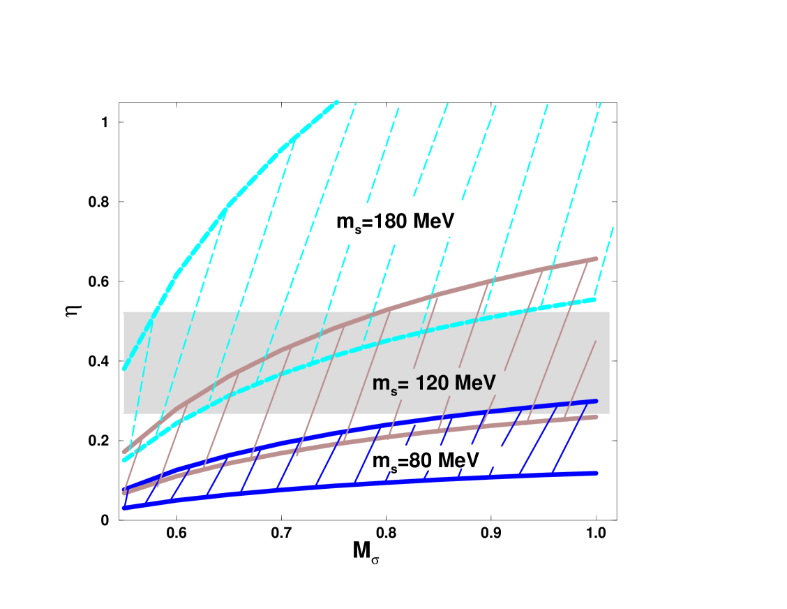
FIG. 1.: Allowed regions for $M_{\sigma}$-$\eta$ from $\epsilon^{\prime}/\epsilon$ data at 2-$\sigma$ confidence level. They are shown for three different values for the strange quark mass, i.e.,$m_{s}$(2GeV)= 80, 120, 180 MeV.

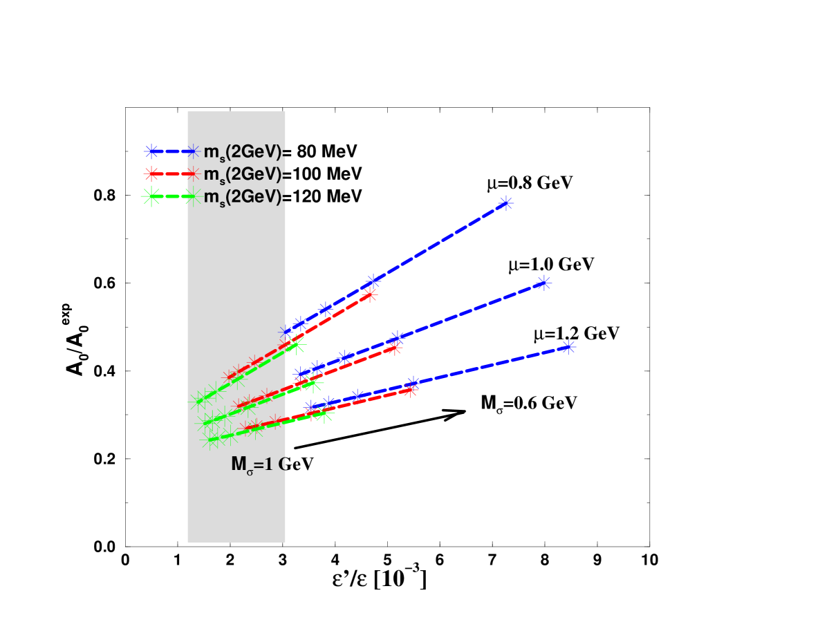
FIG. 2.: Correlation of $a_{0}$ and $\epsilon^{\prime}/\epsilon$. The stars on the lines correspond to $M_{\sigma}$ =0.6, 0.7, 0.8, 0.9, 1.0 GeV, $m_{s}$(2GeV)=80, 100, 120 MeV at factrization scale $\mu$ =0.8, 1.0, 1.2 GeV.

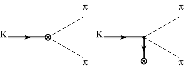
FIG. 3.: Feynman diagrams for $T_{direct}+T_{tadpole}$.

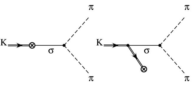
FIG. 4.: Feynman diagrams for $T_{\sigma\mbox{-}pole}+T_{\sigma\mbox{-}tad}$.

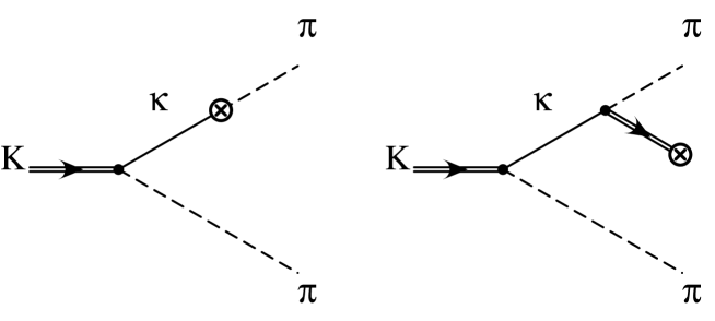
FIG. 5.: Feynman diagrams for $T_{\kappa\mbox{-}pole}+T_{\kappa\mbox{-}tad}$.

	$\pi^{0}\pi^{0}$	$|\pi^{+}>\times|\pi^{-}>$	$|\pi^{0}>\times|\pi^{+}>$
$Q_{1}$	$-X$	$0$	$X/\sqrt{2}$
$Q_{2}$	$0$	$X$	$X/\sqrt{2}$
$Q_{3}$	$0$	$0$	$0$
$Q_{4}$	$X$	$X$	$0$
$Q_{5}$	$0$	$0$	$0$
$Q_{6}$	$Y_{6}$	$Y_{6}$	$0$
$Q_{7}$	$3X/2$	$0$	$-3X/2\sqrt{2}$
$\tilde{Q}_{8}$	$0$	$\tilde{Y}_{8}$	$\tilde{Y}_{8}/\sqrt{2}$
$Q_{9}$	$-3X/2$	$0$	$3X/2\sqrt{2}$
$Q_{10}$	$-X/2$	$X$	$X/\sqrt{2}$
$Q_{11}$	$X$	$0$	$X/\sqrt{2}$

TABLE I.: The matrix elements, where $X=i\sqrt{2}f({M_{k}}^{2}-{M_{\pi}}^{2})$. $\tilde{Y}_{8}$ and $Y_{6}$ are defined in the text.

	$a_{0}$	$a_{2}$
$Q_{1}$	$-\sqrt{1\over 3}X$	$\sqrt{2\over 3}X$
$Q_{2}$	${2\over\sqrt{3}}X$	$\sqrt{2\over 3}X$
$Q_{3}$	$0$	$0$
$Q_{4}$	$\sqrt{3}X$	$0$
$Q_{5}$	$0$	$0$
$Q_{6}$	$\sqrt{3}Y_{6}$	$0$
$Q_{7}$	${\sqrt{3}\over 2}X$	$-\sqrt{3\over 2}X$
$Q_{8}$	${2\over\sqrt{3}}\tilde{Y}_{8}-{\sqrt{3}\over 2}Y_{6}$	${\sqrt{2\over 3}}\tilde{Y}_{8}$
$Q_{9}$	$-{\sqrt{3}\over 2}X$	$\sqrt{3\over 2}X$
$Q_{10}$	${\sqrt{3}\over 2}X$	$\sqrt{3\over 2}X$

TABLE II.: Contribution to isospin amplitudes.

	$M_{\sigma}$ (GeV)	0.55	0.6	0.7	0.8	0.9	1.0
$\Delta=1/20$	$B^{1/2}_{6}$	5.27	3.29	2.22	1.84	1.64	1.52
	$B^{3/2}_{8}$	0.70	0.73	0.77	0.79	0.81	0.82
	$M_{\sigma}$ (GeV)	0.55	0.6	0.7	0.8	0.9	1.0
$\Delta=1/25$	$B^{1/2}_{6}$	4.81	3.06	2.12	1.78	1.61	1.50
	$B^{3/2}_{8}$	0.90	0.93	0.96	0.99	1.00	1.01
	$M_{\sigma}$ (GeV)	0.55	0.6	0.7	0.8	0.9	1.0
$\Delta=1/30$	$B^{1/2}_{6}$	4.48	2.90	2.05	1.75	1.60	1.51
	$B^{3/2}_{8}$	1.13	1.15	1.17	1.19	1.20	1.21

TABLE III.: Bag-factor

Wilson coeff.	$\mu=80.2$ GeV	$\mu=1.2$ GeV	$\mu=1.0$ GeV	$\mu=0.8$ GeV
$y_{1}$	0.0	0.0	0.0	0.0
$y_{2}$	0.0	0.0	0.0	0.0
$y_{3}$	0.0014715	0.03058	0.03335	0.03722
$y_{4}$	-0.0019375	-0.05871	-0.05884	-0.05844
$y_{5}$	0.0006458	0.00311	-0.00168	-0.01384
$y_{6}$	-0.0019375	-0.09797	-0.11672	-0.16226
$y_{7}/\alpha_{QED}$	0.1262367	-0.03714	-0.03822	-0.04038
$y_{8}/\alpha_{QED}$	0.0	0.14352	0.17174	0.23136
$y_{9}/\alpha_{QED}$	-1.0606455	-1.46549	-1.54058	-1.69377
$y_{10}/\alpha_{QED}$	0.9	0.57829	0.68795	0.89882
$z_{1}$	0.0526643	-0.45108	-0.52381	-0.64505
$z_{2}$	0.9812457	1.23913	1.28816	1.37464
$z_{3}$	0.0	0.00674	0.01353	0.03059
$z_{4}$	0.0	-0.01980	-0.03704	-0.07439
$z_{5}$	0.0	0.00569	0.00784	0.00844
$z_{6}$	0.0	-0.01950	-0.03698	-0.08023
$z_{7}/\alpha_{QED}$	0.0	0.00940	0.01249	0.01989
$z_{8}/\alpha_{QED}$	0.0	0.00349	0.01551	0.04725
$z_{9}/\alpha_{QED}$	0.0	0.01127	0.02019	0.03993
$z_{10}/\alpha_{QED}$	0.0	-0.00219	-0.00893	-0.02287

TABLE IV.: List of Wilson coefficients $y_{i},z_{i}$.

REFERENCES

- [1] A. Alavi-Harati et. al. Phys. Rev. Lett. 83, 22 (1999).
- [2] M. S. Sozzi, NA48 experiment at CERN, talk given at Kaon ’99, June 21 (1999).
- [3] A. I. Vainstein, V. I. Zakharov and M. A. Shifman, JETP 45, 670 (1977).
- [4] J. Bijnens and M. B. Wise, Phys. Lett. B137, 245 (1984).
- [5] J. M. Flynn and L. Randall, Phys. Lett. B224, 221 (1989).
-
[6]
C. Dib, I. Dunietz, and F. J. Gilman,
Phys. Lett. B218, 487 (1989),
Phy. Rev. D39, 2639 (1989). - [7] Y.Y. Keum, U. Nierste and A.I. Sanda, Phys. Lett. B457, 157 (1999).
- [8] E.P.Shabalin, Yad. Fiz. 48, 272 (1988) [Sov.J. Nucl. Phys. 48, 404 (1988)].
- [9] T. Morozumi, C. S. Lim and A. I. Sanda, Phys. Rev. Lett. 65, 404 (1990).
-
[10]
M. Harada, F. Sannino and J. Schechter,
Phys. Rev. D54, 1991 (1996);
Phys. Rev. Lett. 78, 1603 (1997). - [11] N. A. Törnqvist and M. Roos, Phys. Rev. Lett. 76, 1575 (1996).
- [12] S. Ishida, M. Y. Ishida, H. Takahashi, T. Ishida, K. Takamatsu and T. Tsuru, Prog. Theor. Phys. 95, 745 (1996).
- [13] D. Morgan and M. Pennington, Phys. Rev. D48, 1185 (1993).
- [14] G. Janssen, B. C. Pearce, K. Holinde and J. Speth, Phys. Rev. D52, 2690 (1995).
- [15] Review of Particle Physics, The European Physical Journal, 3, 363 (1998).
- [16] G. Ecker, J. Gasser, A. Pich and E. De Rafael, Nucl. Phys. B321, 311 (1989).
- [17] G. Ecker, J. Kambor, D. Wyler, Nucl.Phys. B394,101 (1993).
- [18] G. Buchalla, A. J. Buras, and M. E. Lautenbacher, Rev.Mod.Phys. 68, 1125 (1996).
- [19] A. J. Buras, M. Jamin, M. E. Lautenbacher Nucl. Phys. bf B408, 209 (1993).
- [20] G. Buchalla, A. J. Buras, and K. Harlander, Nucl. Phys. B337, 313 (1989).
- [21] W. A. Bardeen, A. J. Buras, and J.-M. Grard, Phys. Lett. B180, 133 (1986).
-
[22]
P. Colangelo, F. De Fazio, G. Nardulli and N. Paver,
Phys. Lett. B408, 340 (1997);
M. Jamin, Nucl. Phys. Proc. Suppl. 64, 250 (1998);
C. A. Dominguez, L. Pirovano and K. Schilcher, Phys. Lett. B425, 193 (1998);
K. Maltman, preprint, hep-ph/9904370;
S. Narison, preprint, hep-ph/9905264;
A. Pich and J. Prades, JHEP 9910, 004 (1999). -
[23]
C. R. Allton et al., Nucl. Phys. B431,667 (1994);
R. Gupta and T. Bhattacharya, Phys. Rev. D55,7203 (1997);
B. J. Gough et al. Phys. Rev. Lett 79, 1622 (1997);
N. Eicker et al., SESAM Collaboration, Phys. Lett.B407,290 (1997);
N. Eicker et al., SESAM Collaboration, Phys. Rev.D 59,014509 (1999);
A. Cucchieri et al., Phys. Lett. B422,212(1998);
M. Gockeler et al., Phys. Rev. D57,5562(1998);
V. Gimenez et al., Nucl. Phys. B540,472(1999);
D. Becirevic et al., Phys. Lett. B444,401(1998);
S. Aoki et al., Phys. Rev. Lett. 82,4392(1999);
S. Aoki et al. UTCCP-P-65, preprint, hep-lat/9904012;
T. Blum, A. Soni, M. Wingate, BNL-HET-99-2, preprint, hep-lat/9902016. -
[24]
R. S. Chivukula, J. M. Flynn and H. Georgi,
Phys. Lett. B171, 453 (1986);
A. J. Buras adn J. -M. Gerard, Phys. Lett. B192, 156 (1987). - [25] W. A. Bardeen, A. J. Buras, and J.-M. Grard, Phys. Lett. B192, 138 (1987).
- [26] A. J. Buras, in CP violation, ed. C.Jarlskog, World Scientific, 575 (1989).
-
[27]
CHPT corrections up to in the chiral quark model
have been discussed in:
S. Bertolini, J.O. Eeg, M. Fabbrichesi, E.I. Lashin, Nucl. Phys. B514, 63-92 and 93-112 (1998). - [28] T. Hambye, G. O. Kohler and P.H.Soldan, Eur. Phys. J. C10, 271-292 (1999).
- [29] T. Hambye, G. O. Kohler, E. A. Paschos, P. H. Soldan , W. A. Bardeen, Phys. Rev. D58, 014017 (1998).