CP Violation in Hyperon Decays from Supersymmetry

Abstract

It was pointed out recently that supersymmetry can generate flavor-changing gluonic dipole operators with sufficiently large coefficients to dominate the observed value of $\epsilon^{\prime}/\epsilon$. We point out that the same operators contribute to direct CP violation in hyperon decay and can generate a CP violating asymmetry $A(\Lambda^{0}_{-})$ in the range probed by the current E871 experiment. Interestingly, models that naturally reproduce the relation $\lambda=\sqrt{m_{d}/m_{s}}$ do not generate $\epsilon^{\prime}/\epsilon$ but could lead to an $A(\Lambda^{0}_{-})$ of $O(10^{-3})$.

The origin of CP violation remains one of the outstanding problems in particle physics. Until recently the only observation of CP violation was in the neutral kaon mixing, with a value of $\epsilon\approx 2.27\times 10^{-3}\exp(i\pi/4)$ [1, 2]. The KTeV and NA48 collaborations have now reported observations of direct CP violation in the neutral kaon decay amplitudes [3], with the world average value being ${\rm Re}(\epsilon^{\prime}/\epsilon)=(21.2\pm 4.6)\times 10^{-4}$ [4].

Although this result is not inconsistent with the standard model prediction, it can be used to constrain other models of CP violation [5, 6, 7]. In particular, it has been found that there can be large supersymmetric contributions to $\epsilon^{\prime}/\epsilon$ [5, 6]. Depending on which new contributions are large, there are different consequences for other processes such as rare kaon decays [8] and hyperon decays.

In this letter we concentrate on the supersymmetric scenario in which the gluonic dipole operators can have large coefficients. In this case there are potentially large contributions to both $\epsilon^{\prime}/\epsilon$ [5] and to the CP violating asymmetry $A(\Lambda^{0}_{-})$ in hyperon non-leptonic decays.

Experiment E871 at Fermilab is expected to reach a sensitivity of $2\times 10^{-4}$ for the observable ($A(\Lambda^{0}_{-})+A(\Xi^{-}_{-})$) [9]. The CP violating asymmetry $A(\Lambda^{0}_{-})$ compares the decay parameter $\alpha$ from the reaction $\Lambda^{0}\rightarrow p\pi^{-}$ to the corresponding parameter $\bar{\alpha}$ in $\bar{\Lambda}^{0}\rightarrow\bar{p}\pi^{+}$ whereas $A(\Xi^{-}_{-})$ is the corresponding asymmetry for the mode $\Xi^{-}\rightarrow\Lambda^{0}\pi^{-}$. These asymmetries have a very simple form when one neglects the small $\Delta I=3/2$ amplitude, for example [10],

$$A(\Lambda^{0}_{-}) = {\alpha+\bar{\alpha}\over\alpha-\bar{\alpha}}\approx-\tan(\delta_{11}-\delta_{1})\sin(\phi_{p}-\phi_{s}),$$ (1)

where $\delta_{1}=6^{\circ}$, $\delta_{11}=-1.1^{\circ}$ are the final state $\pi N$ interaction phases for S and P wave amplitudes with $I=1/2$, respectively [11]. $\phi_{s,p}$ are the corresponding CP violating weak phases. Recent calculations suggest that the strong scattering phases in the $\Lambda^{0}\pi$ final state of the $\Xi$ decay are small [12], and, therefore, the current theoretical prejudice is that $|A(\Lambda^{0}_{-})|$ will dominate the measurement. The standard model prediction for this quantity is around $3\times 10^{-5}$, albeit with large uncertainty [10, 13]. This suggests that a non-zero measurement by E871 will be an indication for new physics.

A model independent study of new CP violating interactions has shown that $A(\Lambda^{0}_{-})$ could be ten times larger than in the standard model and within reach of E871 [14]. A particular example of an operator in which $A(\Lambda^{0}_{-})$ can be this large is precisely the gluonic dipole operator [14]. The results of E871, therefore, can have a direct impact on supersymmetric models.

The short distance effective Hamiltonian for the gluonic dipole operator of interest is,

$${\cal H}_{\it eff} = C_{g}{g_{s}\over 16\pi^{2}}m_{s}\bar{d}\sigma_{\mu\nu}G^{\mu\nu}_{a}t^{a}(1+\gamma_{5})s$$ (3)

$$+\tilde{C}_{g}{g_{s}\over 16\pi^{2}}m_{s}\bar{d}\sigma_{\mu\nu}G^{\mu\nu}_{a}t^{a}(1-\gamma_{5})s~{}+~{}{\rm h.c.},$$

where $Tr(t^{a}t^{b})=\delta^{ab}/2$, and the Wilson coefficients $C_{g}$ and $\tilde{C}_{g}$ that occur in supersymmetry can be found in the literature [15], they are

$$C_{g}=(\delta^{d}_{12})_{LR}{\alpha_{s}\pi\over m_{\tilde{g}}m_{s}}G_{0}(x)\;,\;\tilde{C}_{g}=(\delta^{d}_{12})_{RL}{\alpha_{s}\pi\over m_{\tilde{g}}m_{s}}G_{0}(x).$$ (4)

The parameters $\delta_{12}^{d}$ characterize the mixing in the mass insertion approximation [15], and $x=m_{\tilde{g}}^{2}/m_{\tilde{q}}^{2}$, with $m_{\tilde{g}}$, $m_{\tilde{q}}$ being the gluino and average squark masses, respectively. The loop function is given by,

$$G_{0}(x)=x{22-20x-2x^{2}+(16x-x^{2}+9)\log x\over 3(x-1)^{4}}.$$ (5)

Ref. [8] has noted that, in this form, $G_{0}(1)=-5/18$ and the function does not depend strongly on $x$. The effect of QCD corrections is to multiply the Wilson coefficients by [16]

$$\eta=\biggl{(}{\alpha_{s}(m_{\tilde{g}})\over\alpha_{s}(m_{t})}\biggr{)}^{2\over 21}\biggl{(}{\alpha_{s}(m_{t})\over\alpha_{s}(m_{b})}\biggr{)}^{2\over 23}\biggl{(}{\alpha_{s}(m_{b})\over\alpha_{s}(m_{c})}\biggr{)}^{2\over 25}.$$ (6)

To calculate the weak phases we adopt the usual procedure of taking the real part of the amplitudes from experiment and of using a model for the hadronic matrix elements to obtain the imaginary part. We use the MIT bag model matrix elements of Ref. [10, 17] to find for the weak phases

$$\phi_{s} = -2.9\times 10^{7}~{}{\rm GeV}$$ (8)

$${\alpha_{s}\over 32\pi}{\eta\over m_{\tilde{g}}}G_{0}(x){\rm Im}\biggl{(}(\delta_{12}^{d})_{LR}-(\delta_{12}^{d})_{RL}\biggr{)}B_{s},$$

$$\phi_{p} = -3.4\times 10^{7}~{}{\rm GeV}$$ (10)

$${\alpha_{s}\over 32\pi}{\eta\over m_{\tilde{g}}}G_{0}(x){\rm Im}\biggl{(}(\delta_{12}^{d})_{LR}+(\delta_{12}^{d})_{RL}\biggr{)}B_{p}.$$

We have introduced the parameters $B_{s}$ and $B_{p}$ to quantify the uncertainty in these matrix elements. We then find,

$$A(\Lambda^{0}_{-})_{SUSY}=\left({\alpha_{s}(m_{\tilde{g}})\over\alpha_{s}(500~{}{\rm GeV})}\right)^{23\over 21}\left({500~{}{\rm GeV}\over m_{\tilde{g}}}\right){G_{0}(x)\over G_{0}(1)}$$ (12)

$$\left((2.0B_{p}-1.7B_{s}){\rm Im}(\delta_{12}^{d})_{LR}+(2.0B_{p}+1.7B_{s}){\rm Im}(\delta_{12}^{d})_{RL}\right).$$

The matrix element of the gluonic dipole operator of Eq. (3) between two baryon states is calculated with the MIT bag model in Ref. [17], and we assume that this result is accurate to within factors of two. The S-wave hyperon decay amplitude is then obtained by using a soft pion theorem which can have $20-30\%$ corrections. The P-wave hyperon decay amplitude is obtained by considering baryon and kaon pole diagrams. A leading order calculation of the dominant, CP conserving, P-wave amplitudes in terms of (octet) baryon poles alone works reasonably well for $\Lambda^{0}$ decays. However, additional contributions are needed to explain the P-waves in other hyperon decays [18], and the first non-leading corrections to the $\Lambda^{0}$ decay amplitude are large. An example of an additional contribution is the kaon pole, which in Eq. (10) accounts for about 20% of the P-wave phase. To reflect these uncertainties in our numerical analysis we use $0.5<B_{s}<2.0$, while allowing $B_{p}$ to vary in the range $0.7B_{s}<B_{p}<1.3B_{s}$.

In a general supersymmetric model there are also contributions to the imaginary parts of the Wilson coefficients of four-quark operators. Of these, the dominant contribution to the CP asymmetry in hyperon decays (within the standard model) is due to $O_{6}$ [13]. We have checked numerically, that SUSY contributions to $C_{6}$ (as well as to $C_{3,4,5,7}$) are much smaller than those in Eq. (LABEL:cpasym), for a parameter range similar to that considered in Ref. [15].

Although the asymmetry $A(\Lambda^{0}_{-})$ is due to the same $|\Delta S|=1$ interaction responsible for $\epsilon^{\prime}/\epsilon$, the two observables are qualitatively different. For $\epsilon^{\prime}/\epsilon$, both the $\Delta I=1/2$ and the $\Delta I=3/2$ amplitudes are equally important, whereas for $A(\Lambda^{0}_{-})$ only the $\Delta I=1/2$ amplitude is important. In this case, the interference necessary for CP violation takes place between $S$ and $P$ waves within the $\Delta I=1/2$ transition. This sensitivity to differences between $S$ and $P$ waves accounts for the different coefficients multiplying $(\delta_{12}^{d})_{LR}$ and $(\delta_{12}^{d})_{RL}$ respectively in Eq. (LABEL:cpasym). For this same reason, supersymmetric scenarios in which $\epsilon^{\prime}$ is enhanced through $\Delta I=3/2$ operators [6, 8] do not enhance $A(\Lambda^{0}_{-})$.

In order to quantify $A(\Lambda^{0}_{-})$ in supersymmetric models where the operators in Eq. (3) have large coefficients, we compare Eq. (LABEL:cpasym) with their contributions to $\epsilon^{\prime}/\epsilon$ [8],

$$\biggl{(}{\epsilon^{\prime}\over\epsilon}\biggr{)}_{SUSY}=\biggl{(}{\alpha_{s}(m_{\tilde{g}})\over\alpha_{s}(500~{}{\rm GeV})}\biggr{)}^{23\over 21}\biggl{(}{500~{}{\rm GeV}\over m_{\tilde{g}}}\biggr{)}{G_{0}(x)\over G_{0}(1)}B_{G}$$ (15)

$$\biggl{(}{158~{}{\rm MeV}\over m_{s}(m_{c})+m_{d}(m_{c})}\biggr{)}58\ {\rm Im}\biggl{(}(\delta_{12}^{d})_{LR}-(\delta_{12}^{d})_{RL}\biggr{)}\ .$$

To obtain this expression, Ref. [8] uses the $K\rightarrow\pi\pi$ matrix element from a chiral quark model calculation in Ref. [19] and uses the parameter $B_{G}$ to quantify the hadronic uncertainty. We use the range $0.5<B_{G}<2$ motivated by the bag model result of Ref. [20] and the dimensional analysis estimate of Ref. [21]. It is interesting to note that $(\epsilon^{\prime}/\epsilon)_{SUSY}$ depends on the same combination of the mass insertion parameters as the weak phase $\phi_{s}$ in Eq. (8). We require $(\epsilon^{\prime}/\epsilon)_{SUSY}$ to be equal to the observed value (i.e., $\epsilon^{\prime}/\epsilon$ dominated by supersymmetry) or less (i.e., $\epsilon^{\prime}/\epsilon$ dominated by the standard model).

Comparing Eqs. (LABEL:cpasym) and (15) one sees that $\epsilon^{\prime}/\epsilon$ and $A(\Lambda^{0}_{-})$ are proportional to different combinations of the coefficients $(\delta_{12}^{d})_{LR}$ and $(\delta_{12}^{d})_{RL}$. For this reason one cannot determine the allowed range for $A(\Lambda^{0}_{-})$ solely in terms of $\epsilon^{\prime}/\epsilon$. In what follows, we consider the three cases: a) ${\rm Im}(\delta_{12}^{d})_{RL}=0$, b) ${\rm Im}(\delta_{12}^{d})_{LR}=0$, and c) ${\rm Im}(\delta_{12}^{d})_{RL}={\rm Im}(\delta_{12}^{d})_{LR}$ motivated below.

It is useful to recall the origin of the mass insertion parameters $(\delta_{12}^{d})_{RL}$ and $(\delta_{12}^{d})_{LR}$. They are the mismatch between the quark mass matrix and left-right mass-squared matrix for down-type squarks (we restrict our discussion to the first and second generations). In many theories of flavor with approximate flavor symmetries, the Cabibbo angle originates in the down-quark sector, and we find the mass matrix to be of the form

$$M_{d}=\left(\begin{array}[]{cc}am_{s}\lambda^{2}&m_{s}\lambda\\ bm_{s}\lambda&m_{s}\end{array}\right),$$ (16)

where $a$ and $b$ are $O(1)$ coefficients and $\lambda$ is the sine of the Cabibbo angle. The (2,2) element is nothing but the strange quark mass itself (ignoring $O(\lambda^{2})$ corrections), and the (1,2) element is fixed by the requirement that the Cabibbo angle is reproduced. The down quark mass is given by $m_{d}=(a-b)\lambda^{2}$. A case of $a=0$ and $b=-1$ naturally reproduces the phenomenologically successful relation $\lambda\simeq\sqrt{m_{d}/m_{s}}$ and deserves a special attention. This arises if the off-diagonal elements originate in an anti-symmetric matrix such as in U(2) model [22]. The $\lambda$ dependence of each element is a consequence of the approximate flavor symmetry, but the constants $a$ and $b$ cannot be determined by symmetry considerations alone and hence are model-dependent. The same approximate flavor symmetry constrains the form of the left-right mass-squared matrix. Therefore, the left-right mass-squared matrix for down-type squarks is

$$M^{2d}_{LR}=m_{SUSY}\left(\begin{array}[]{cc}\tilde{a}m_{s}\lambda^{2}&\tilde{c}m_{s}\lambda\\ \tilde{b}m_{s}\lambda&\tilde{d}m_{s}\end{array}\right),$$ (17)

where $m_{SUSY}$ is the typical supersymmetry breaking scale which we take to be the same as the down-type squark mass, and $\tilde{a}$, $\tilde{b}$, $\tilde{c}$, and $\tilde{d}$ are $O(1)$ numbers and can be complex. The U(2) model gives $\tilde{b}=-\tilde{c}$.

After diagonalizing the quark mass matrix Eq. (16), the left-right mass-squared matrix becomes

$$m_{SUSY}m_{s}\left(\begin{array}[]{cc}(\tilde{a}-b\tilde{c}-\tilde{b}+b\tilde{d})\lambda^{2}&(\tilde{c}-\tilde{d})\lambda\\ (\tilde{b}-b\tilde{d})\lambda&\tilde{d}\end{array}\right).$$ (18)

Unless special relations hold between $O(1)$ coefficients, there remain off-diagonal elements which contribute to flavor-changing neutral currents. The mass insertion parameters for $s\rightarrow d$ transition are defined as

$$(\delta_{12}^{d})_{LR}=\frac{m_{s}(\tilde{c}-\tilde{d})}{m_{SUSY}},$$ (19)

$$(\delta_{12}^{d})_{RL}=(\delta_{21}^{d})_{LR}^{*}=\frac{m_{s}(\tilde{b}-b\tilde{d})^{*}}{m_{SUSY}}.$$ (20)

It is amusing that the size of the mass insertion parameters given here generates $\epsilon^{\prime}$ according to Eq. (15) at the observed level for $m_{SUSY}\sim 500$ GeV and a phase of $O(1)$.

The case a), of ${\rm Im}(\delta_{12}^{d})_{LR}\neq 0$ and ${\rm Im}(\delta_{12}^{d})_{RL}=0$, corresponds to the choice $a=1$, $b=0$ in the quark mass matrix Eq. (16) and its counter part in the squark mass matrix Eq. (17) $\tilde{b}=0$ is also likely to be zero in this case. We still expect $\tilde{c}$, $\tilde{d}$ to be $O(1)$ and this case is the most conservative one. The case b) is the other possible limit where $\tilde{c}-\tilde{d}$ happens to have a negligible imaginary part. ${\rm Im}(\tilde{b}-b\tilde{d})$ can still generate an interesting contribution to $\epsilon^{\prime}$, while $A(\Lambda^{0}_{-})$ can be much larger in this case. Finally, the case c) ${\rm Im}(\delta_{12}^{d})_{RL}={\rm Im}(\delta_{12}^{d})_{LR}$ is motivated by the phenomenological relation $\lambda\simeq\sqrt{m_{d}/m_{s}}$ and hence $a=0$, $b=-1$. The anti-symmetry in $M_{d}$ could imply the anti-symmetry in $M^{2d}_{LR}$, and hence $\tilde{b}=-\tilde{c}$. This is indeed what happens in the U(2) model of flavor [22]. In this case, ${\rm Im}(\delta_{12}^{d})_{LR}=m_{s}{\rm Im}(-\tilde{b}-\tilde{d})/m_{SUSY}$, while ${\rm Im}(\delta_{12}^{d})_{RL}=m_{s}{\rm Im}(\tilde{b}+\tilde{d})^{*}/m_{SUSY}=m_{s}{\rm Im}(-\tilde{b}-\tilde{d})/m_{SUSY}={\rm Im}(\delta_{12}^{d})_{LR}$. Therefore, there is no parity violation in the CP-violating part of the operators and hence the contribution to $\epsilon^{\prime}$ identically vanishes [23]. In this case, the only constraint on the size of $A(\Lambda^{0}_{-})$ comes from $\epsilon$ as we will discuss below.

The operators in Eq. (3) also contribute to $\epsilon$ through long distance effects and we must check that this contribution is not too large. The simplest long distance contributions arise from $\pi^{0}$, $\eta$ and $\eta^{\prime}$ poles as noted in Ref. [24]. They yield,

$$\bigl{(}\epsilon\bigr{)}_{SUSY} = {1\over\sqrt{2}m_{K}\Delta m}{1\over m_{K}^{2}-m_{\pi}^{2}}$$ (22)

$${\rm Im}(\langle\pi^{0}|{\cal H}_{\it eff}|K^{0}\rangle)\langle\pi^{0}|{\cal H}_{SM}|K^{0}\rangle\kappa.$$

In this expression $\Delta m$ is the $K_{L}-K_{S}$ mass difference and $\langle\pi^{0}|{\cal H}_{SM}|K^{0}\rangle\approx 2.6\times 10^{-8}~{}{\rm GeV}^{2}$ is extracted from $K\rightarrow\pi\pi$ data. We get the matrix element $\langle\pi^{0}|{\cal H}_{\it eff}|K^{0}\rangle$ using the MIT bag model result [17]. Finally, $\kappa$ quantifies the contributions of the different poles, $\kappa=1$ corresponding to the pion pole. In the model of Ref. [25] $\kappa\sim 0.2$ whereas the contribution of the $\eta^{\prime}$ alone gives $\kappa\sim-0.9$ [10]. We use $0.2<|\kappa|<1.0$ and demand that this long distance contribution to $\epsilon$,

$$\bigl{(}\epsilon\bigr{)}_{SUSY} = \biggl{(}{\alpha_{s}(m_{\tilde{g}})\over\alpha_{s}(500~{}{\rm GeV})}\biggr{)}^{23\over 21}\biggl{(}{500~{}{\rm GeV}\over m_{\tilde{g}}}\biggr{)}\ {\kappa\over 0.2}\ {G_{0}(x)\over G_{0}(1)}$$ (24)

$$6.4\ {\rm Im}\biggl{(}(\delta_{12}^{d})_{LR}+(\delta_{12}^{d})_{RL}\biggr{)},$$

be smaller than $2.3\times 10^{-3}$. This leads to the constraint $|A(\Lambda^{0}_{-})|<7.3\times 10^{-4}B_{p}$. Note that we allowed the range $0.35<B_{p}<2.6$, and hence $|A(\Lambda^{0}_{-})|$ can be $O(10^{-3})$; we cannot exclude it up to $1.9\times 10^{-3}$. The constraint on the mass insertion parameters from the short-distance effect (e.g., box diagrams) is weaker: $({\rm Im}(\delta_{12}^{d})_{LR}^{2})^{1/2}<3.7\times 10^{-3}$ for $m_{\tilde{g}}=m_{\tilde{q}}=500$ GeV and $(\delta_{12}^{d})_{LR}=(\delta_{12}^{d})_{RL}$ [26].

The regions allowed by the three cases discussed above are shown in Fig. 1. The case a) with LR contribution only is the horizontally-hatched region with the central value shown as a solid line, and the case b) with RL contribution only is the diagonally-hatched region with the central value shown as a solid line. The shaded region at the top is excluded by the $\epsilon$ constraint, and is particularly important for case c) in which there is no contribution to $\epsilon^{\prime}$. It is interesting that the best motivated case c) allows a large asymmetry in hyperon decay. The vertical band shows the world average for $\epsilon^{\prime}/\epsilon$ and the region to the right of the band is, therefore, not allowed.

In summary, we have studied the supersymmetric contribution to CP violation in hyperon decays from gluonic dipole operators. We parameterize the hadronic uncertainties with the quantities $B_{G}$, $B_{s}$, $B_{p}$ and $\kappa$ which we allow to vary in reasonable ranges. We constrain the size of the coefficients of the gluonic dipole operators with the observed value of $\epsilon^{\prime}$ and predict a range for $A(\Lambda^{0}_{-})$ depending on whether the LR or the RL operator dominates. We find that the size of $A(\Lambda^{0}_{-})$ can be within reach of the E871 experiment. Particularly interesting is the scenario c), which explains naturally the relation $\lambda=\sqrt{m_{d}/m_{s}}$. This scenario does not generate $\epsilon^{\prime}$, but it can lead to an $A(\Lambda^{0}_{-})$ as large as $10^{-3}$.

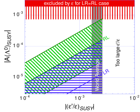
FIG. 1.: The allowed regions on $(|(\epsilon^{\prime}/\epsilon)_{SUSY}|,$ $|A(\Lambda^{0}_{-})_{SUSY}|)$ parameter space for three cases: a) only ${\rm Im}(\delta^{d}_{12})_{LR}$ contribution, which is the conservative case (hatched horizontally), b) only ${\rm Im}(\delta^{d}_{12})_{RL}$ contribution (hatched diagonally), and c) ${\rm Im}(\delta^{d}_{12})_{LR}={\rm Im}(\delta^{d}_{12})_{RL}$ case which does not contribute to $\epsilon^{\prime}$ and can give a large $|A(\Lambda^{0}_{-})|$ below the shaded region (or vertically hatched region for the central values of the matrix elements). The last case is motivated by the relation $\lambda=\sqrt{m_{d}/m_{s}}$. The vertical shaded band is the world average [4] of $\epsilon^{\prime}/\epsilon$. The region to the right of the band is therefore not allowed.

REFERENCES

[1] J. Christenson et al.,Phys. Rev. Lett. 13, 138 (1964).
[2] Particle Data Book, Eur. Phys. J. C3, 1 (1998).
[3] KTeV Collaboration,
A. Alavi-Harati et. al., Phys. Rev. Lett. 83, 22 (1999);
NA48 Collaboration, V. Fanti et. al., CERN-EP/99-114, hep-ex/9909022.
[4] This is the average of E731, NA31, KTeV and NA48 with the
error bar inflated to obtain according to
the Particle Data Group prescription.
[5] A. Masiero and H. Murayama, Phys. Rev. Lett. 83, 907
(1999);
K.S. Babu, B. Dutta and R. Mohapatra, e-print hep-ph/9905464;
S. Khalil and T. Kobayashi, Phys. Lett. B460 341 (1999);
S. Baek et. al., e-print hep-ph/9907572;
G. Eyal et. al., e-print hep-ph/9908382.
[6] A. L. Kagan and M. Neubert, hep-ph/9908404.
[7] X.-G. He, Phys. Lett. B460, 405 (1999);
D. Chang, X.-G. He and B. McKellar, hep-ph/9909357.
[8] G. Colangelo and G. Isidori, JHEP 9809 009A (1998);
A. Buras, et. al., e-print hep-ph/9908371; G. Colangelo,
G. Isidori, and J. Portoles, e-print hep-ph/9908415.
[9] C. White, et. al., Nucl. Phys. Proc.
Suppl. B71, 451 (1999).
[10] J. Donoghue and S. Pakvasa, Phys. Rev. Lett. 55, 162 (1985);
J. Donoghue, X.-G. He and S. Pakvasa, Phys. Rev. D34, 833 (1986).
[11] L. D. Roper, R. M. Wright and B. Feld,
Phys. Rev. 138, 190 (1965); A. Datta and S. Pakvasa, Phys. Rev.
D56, 4322 (1997).
[12] M. Lu, M. Savage and M. Wise, Phys. Lett. B337,
133 (1994); A. Datta and S. Pakvasa, Phys. Lett. B344, 430 (1995);
A. Kamal, Phys. Rev. D58, 077501 (1998); J. Tandean and G. Valencia,
Phys. Lett. B451, 382 (1999).
[13] X.-G. He, H. Steger, and G. Valencia, Phys. Lett. B272,
411 (1991).
[14] X.-G. He and G. Valencia, Phys. Rev. D52, 5257 (1995).
[15] F. Gabbiani et al.,
Nucl. Phys. B447, 321 (1996).
[16] M. Ciuchini et al., Phys. Lett. B316, 127 (1993);
M. Ciuchini et al., Nucl. Phys. B421, 41 (1994).
[17] J. Donoghue et. al., Phys. Rev. D23, 1213
(1981).
[18] J. Donoghue, E. Golowich and B. Holstein,
Dynamics of the Standard Model, Cambridge University Press, (1992).
[19] S. Bertolini, J. Eeg and M. Fabbrichesi, Nucl. Phys.
B449, 197 (1995).
[20] J. Donoghue and B. Holstein, Phys. Rev. D32,
1152 (1985).
[21] X.-G. He and G. Valencia, hep-ph/9909399.
[22] R. Barbieri, G. Dvali and L.J. Hall, Phys. Lett. B377, 76 (1996); R. Barbieri, L.J. Hall, and A. Romanino,
Phys. Lett. B401, 47 (1997).
[23] The authors of R. Barbieri, R. Contino, and A. Strumia,
hep-ph/9908255 initially had a different conclusion, but now agree with our
analysis and have revised their paper accordingly. We thank R. Barbieri for
communications.
[24]
J. Donoghue and B. Holstein, Phys. Rev. D32, 1152 (1985);
H.-Y. Cheng, Phys. Rev. D34, 1397 (1986);
[25]J. Donoghue, B. Holstein and Y. Lin, Nucl. Phys. B277,
651 (1986).
[26] M. Ciuchini et al, JHEP 10 008 (1998).