Static Potential in the SU(2)-Higgs Model and the Electroweak Phase Transition

Abstract

We present a one-loop calculation of the static potential in the SU(2)-Higgs model. The connection to the coupling constant definition used in lattice simulations is clarified. The consequences in comparing lattice simulations and perturbative results for finite temperature applications are explored.

1 Introduction

One of the most fundamental and intriguing problems in present-day particle physics is the observed baryon asymmetry of the universe—that is the fact that we do not see hardly any antimatter around us, but we can see a large amount of matter, and a vast amount of photons.

One could be inclined to attribute this asymmetry to the initial conditions of the big bang—but this being rather ad hoc, we shall focus on dynamical generation of baryons. Another possibility could be arguing that the entire universe has no net baryon number, just our region is more baryonic, while other regions are more antibaryonic. However, from the boundary between two such regions, characteristic photons would bring us information, and lacking this, we can safely state that in our vicinity of at least $10^{13}$ solar masses there is just matter. Since no known mechanism can separate matter and antimatter on such large scales, we shall assume that the universe is baryonic and this asymmetry was formed some time after the big bang.

In 1967 Sakharov gave three necessary conditions for baryogenesis, which are

1. Baryon number violation—which is obvious

2. C and CP violation—otherwise the number of baryons and antibaryons generated would be equal

3. Departure from thermal equilibrium—since quantum numbers do not change in thermal equilibrium

Baryon number violating processes are known to be present in GUT’s—and GUT’s are still favoured candidates for baryogenesis. However, it came as a slight surprise that even within the standard model there are such processes, the nonperturbative sphaleron processes. The standard model being experimentally verified with great precision, the investigation of the possibility of electroweak baryogenesis is clearly of great importance.

The departure from thermal equilibrium can be realised during the electroweak phase transition. This is customarily described by the effective potential.

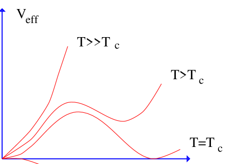
Figure 1: The effective potential as a function of the scalar field. The phase transition point is defined by the degeneracy of the two minima

In order to have electroweak baryogenesis, the phase transition must be strongly first order, or more quantitatively the relation

$$\langle\Phi\rangle/T_{C}>1$$

must hold, i.e. the vev of the Higgs field has to exceed the critical temperature.

How can we study this relation? The most straightforward method is resummed perturbation theory (cf. e.g. [1, 2, 3]). In the low temperature Higgs phase the perturbative approach is expected to work well, however, serious infrared problems are present in the high temperature symmetric phase. Since the determination of thermodynamical quantities at the critical temperatures is based on the properties of both phases, non-perturbative techniques are necessary for a quantitative understanding of the phase transition.

One very successful possibility is to construct an effective 3-dimensional theory by using dimensional reduction, which is a perturbative step. The non-perturbative study is carried out in this effective 3-dimensional model (see e.g. [4] and references therein). Analytical estimates are confirmed by numerical results and relative errors are believed to be at the percent level.

Another approach is to use 4-dimensional simulations. The complete lattice analysis of the standard model is not feasible due to the presence of chiral fermions. however, the infrared problems are connected only with the bosonic sector. These are the reasons why the problem is usually studied by simulating the SU(2)-Higgs model on 4-dimensional lattices, and perturbative steps are used to include the U(1) gauge group and the fermions.

Despite the fact that both perturbative and lattice approaches are systematic and well-defined, it is not easy to compare their predictions. The reason for this is that in lattice simulations the gauge coupling constant is determined from the static potential, whereas in perturbation theory the ${\overline{\rm{MS}}}$ scheme is used. Therefore, if one wishes to compare perturbative and lattice results, a perturbative calculation of the static potential proves to be of great help.

2 Calculation of the one-loop static potential

The concept of the static potential was introduced more than 20 years ago by L. Susskind [5].

Figure 2: Heavy quark–antiquark loop

When a very heavy quark–antiquark pair is created from vacuum, separated and kept at distance $r$ for time $t$ and then let annihilate, the matrix element of the process can be given as

$$\langle i|e^{-Ht}|f\rangle=e^{-V(r)t}\langle i|f\rangle,$$

and so

$$V(r)=-\lim_{t\to\infty}\frac{1}{t}\log\langle W_{r,t}\rangle.$$ (1)

The Feynman rules for these static sources are quite simple. Owing to their great mass, their coordinate space propagator is purely timelike,

$$iS_{Q/A}(x-y)=\delta({\mathbf{x-y}})\theta(\pm x_{0}\mp y_{0}),$$

which upon Fourier transformation gives the momentum space propagator

$$iS_{Q/A}^{ab}(p)\displaystyle\frac{i}{vp+i\epsilon},$$

where $v$ is the velocity of the source ([1,0,0,0] to a first approximation).

The heavy (anti)quark–gauge boson vertex is given by

$$V_{Q/A}^{a,\mu}=\pm igT^{a}_{i,j}\delta^{\mu 0}$$

By means of these rules, the one-loop static potential was calculated long ago in quantum electrodynamics and quantum chromodynamics [5, 6, 7], and even the full two-loop result was published recently [8]. The case of QED is rather simple: it was shown in [6] that summing up all orders in perturbation theory is equivalent to taking the exponential of the one gauge boson exchange graph. However, this calculation is more than just a warm-up excercise, as the abelian parts of the graphs in more complicated theories (QCD, SU(2)-Higgs model) are identical to those of QED. Therefore we can focus on graphs with nonabelian contributions.

Our calculation was performed in the ${\overline{\rm{MS}}}$ scheme and the Feynman gauge but the result is gauge independent, as it should be for a physical observable. The relevant graphs are shown in Fig. 3.

Solid lines represent the heavy quark (antiquark) propagator, while wavy lines the vector boson propagator. External heavy quark (antiquark) propagators are not shown in the figure. The one-loop corrected vector boson propagator contains scalar and ghost contributions as well. The result can be conveniently given in momentum space. One obtains [9, 10]

$$\displaystyle{V_{{\mathrm{1-loop}}}(k)=-\frac{3g^{4}}{32\pi^{2}}\frac{1}{k^{2}+M_{W}^{2}}}$$

$$\displaystyle{\left\{\frac{k^{2}+M_{W}^{2}}{k}\frac{2}{\sqrt{k^{2}+4M_{W}^{2}}}\log\frac{\sqrt{k^{2}+4M_{W}^{2}}-k}{\sqrt{k^{2}+4M_{W}^{2}}+k}+\right.}$$

$$\displaystyle{\frac{1}{k^{2}+M_{W}^{2}}\left[\frac{1}{24R_{HW}^{2}}\left(86R_{HW}^{2}k^{2}-9(6-3R_{HW}^{2}+R_{HW}^{4})M_{W}^{2}\right)\log\frac{\mu^{2}}{M_{W}^{2}}\right.}$$

$$\displaystyle{+\frac{1}{8}(13k^{2}-20M_{W}^{2})F(k^{2};M_{W}^{2},M_{W}^{2})}$$

$$\displaystyle{-\frac{1}{24}\left((R_{HW}^{2}-1)^{2}\frac{M_{W}^{4}}{k^{2}}+k^{2}+2(R_{HW}^{2}-5)M_{W}^{2}\right)F(k^{2};M_{W}^{2},M_{H}^{2})}$$

$$\displaystyle{+\frac{R_{HW}^{2}\cdot\log R_{HW}}{12(R_{HW}^{2}-1)}\left(k^{2}+(9R_{HW}^{2}-17)M_{W}^{2}\right)}$$

$$\displaystyle{\left.\left.+\frac{1}{72R_{HW}^{2}}\left(R_{HW}^{2}k^{2}+3(-18+R_{HW}^{2}-11R_{HW}^{4})M_{W}^{2}\right)\right]\right\}},$$ (2)

where $k^{2}$ denotes the square of the three-momentum $\vec{k}$, $M_{H}$ the Higgs mass and $R_{HW}=M_{H}/M_{W}$. The function $F$ is defined as

$$F(k^{2};m_{1}^{2},m_{2}^{2})=1+\frac{m_{1}^{2}+m_{2}^{2}}{m_{1}^{2}-m_{2}^{2}}\log\frac{m_{1}}{m_{2}}+\frac{m_{1}^{2}-m_{2}^{2}}{k^{2}}\log\frac{m_{1}}{m_{2}}$$

$$+\frac{1}{k^{2}}\sqrt{(m_{1}+m_{2})^{2}+k^{2})((m_{1}-m_{2})^{2}+k^{2})}\log\displaystyle{\frac{1-\sqrt{\frac{(m_{1}-m_{2})^{2}+k^{2}}{(m_{1}+m_{2})^{2}+k^{2}}}}{1+\sqrt{\frac{(m_{1}-m_{2})^{2}+k^{2}}{(m_{1}+m_{2})^{2}+k^{2}}}}}.$$ (3)

Although the dependence on the renormaization scale can be removed by introducing the one-loop W mass [10], we do not follow this line.

Eq. (2) has to be Fourier transformed into coordinate space. We applied brute force methods performing numerical integration. As a check, we compared our results with various pieces of the partly analytic calculation in [10] for the derivative of the potential (with respect to distance). The agreement is excellent.

Figure 3: Graphs giving nonvanishing contributions to the static potential

Our result is presented in Figs. 2 and 3, where the various parts of the one-loop correction to the potential are plotted. We define

$$\frac{V(r)}{M_{W}}=-\frac{3g^{2}}{16\pi}\frac{\exp(-M_{W}^{0}r)}{M_{W}r}+\frac{g^{4}}{16\pi^{2}}\left(A+B\log(\mu^{2}/M_{W}^{2})\right),$$ (4)

where $M_{W}^{0}=M_{W}-\delta M_{W}$, with $\delta M_{W}$ the one-loop mass correction. Since $\delta M_{W}$ is scale dependent, so is $M_{W}^{0}$. A and B are functions of the distance $r$ and $R_{HW}=M_{H}/M_{W}$. We choose $M_{W}=80$GeV. Fig. 4 shows the dependence of $A$ and $B$ on the dimensionless distance $rM_{W}$ for $R_{HW}=0.8314$ (corresponding to the end point of the first order finite temperature phase transition [11]), while Fig. 5 shows the $R_{HW}$ dependence for $r=M_{W}^{-1}$.

Figure 4: The coefficients of $g^{4}/(16\pi^{2})$—curve A—and of $g^{4}/(16\pi^{2})\log(\mu^{2}/M_{W}^{2})$—curve B—of the static potencial Eq. (4) as a function of distance times W mass. $R_{HW}$=0.8314.

Figure 5: The coefficients of $g^{4}/(16\pi^{2})$—curve A—and of $g^{4}/(16\pi^{2})\log(\mu^{2}/M_{W}^{2})$—curve B—of the static potencial Eq. (4) as a function of $R_{HW}$. The distance is $M_{W}^{-1}$.

3 Relation of the continuum version of the lattice coupling constant definition to the ${\mathbf{\overline{\mathbf{MS}}}}$ coupling constant

Since we wish to compare results of lattice simulations and continuum perturbation theory calculations, it is an essential point to define the SU(2) gauge coupling in the same way in both cases. However, in continuum perturbation theory the $\overline{\rm{MS}}$ running coupling constant at a given renormalization scale is more natural (as used in Eqs. (2,4), too), while in lattice simulations other definitions are applied. Therefore we have to establish the relation between the coupling constants.

The lattice definition of the coupling constant (inspired by [12]) is given in [13].

First rectangular Wilson loops of size $(r,t)$ are measured. Extrapolating to large $t$ and dividing the logarithm by $-t$ one gets the static potential in the $t\rightarrow\infty$ limit as a function of $r$ [see Eq. (1)]. The nonperturbative lattice static potential is fitted by a finite lattice version of the Yukawa potential with four parameters (for details cf. [13]). One of these parameters is the mass in the exponential of the Yukawa potential, which is usually called the screening mass. The gauge coupling at distance $r$ is defined as the ratio of the discrete $r$ derivative of the lattice simulated nonperturbative potential and the discrete derivative of the tree-level lattice Yukawa potential normalized by the square of the tree-level coupling and with the mass parameter $M_{\mathrm{lattice}}$ identified with the screening mass. In practice $g^{2}_{\mathrm{lattice}}(M_{\mathrm{lattice}}^{-1})$ is determined and is called the local renormalized gauge coupling constant on the lattice. The lattice results at various Higgs masses are collected in Table 1. Data are from [11, 13, 14, 15].

The gauge coupling constant can be defined in the same spirit in the case of continuum perturbation theory, too:

$$g_{R}^{2}(r)=\frac{1}{C_{F}}\frac{\displaystyle\frac{d}{dr}\left[-V(r)\right]}{\displaystyle\frac{d}{dr}\int\frac{d^{3}k}{(2\pi)^{3}}\frac{\exp(i{\vec{k}}\cdot{\vec{r}})}{k^{2}+M_{\rm screen}^{2}}},$$ (5)

i.e. by taking the ratio of the derivatives with respect to $r$ of the one-loop potential and the tree-level potential normalized by the square of the tree-level coupling. In Eq. (5) $V(r)$ is given by Eq. (4), $C_{F}=3/4$, and $M_{\rm screen}$ is obtained from the fit.

Since $M_{\rm screen}-M_{W}^{0}=O(g^{2})$, for distances satisfying $M_{\rm screen}-1/r=O(g^{2})$ we can put Eq. (5) into the form

$$g_{R}^{2}(r)=g_{\overline{\rm{MS}}}^{2}(\mu)\left(1+\frac{1}{2}\left(1-\frac{M_{W}^{0}}{M_{\rm screen}}\right)\right)+\frac{g_{\overline{\rm{MS}}}^{4}(\mu)}{16\pi^{2}}\left(C+D\log\frac{\mu^{2}}{M_{W}^{2}}\right).$$ (6)

$C$ and $D$ are functions of $R_{HW}$ and $M_{\rm screen}$, their values are tabulated in Table 2 for $M_{\rm screen}=M_{W}=80$GeV.

$R_{HW}$	.2049	.4220	.595	.8314
$T_{C}$ (GeV)	38.3	72.6	100.0	128.4
$M_{\mathrm{lattice}}$ (GeV)	84.3(12)	78.6(2)	80.0(4)	76.7(24)
$g^{2}_{\mathrm{lattice}}(M^{-1})$	.5630(60)	.5788(16)	.5782(25)	.569(4)
$M_{\rm screen}$ (GeV)	74.97	80.44	80.70	81.77
$g^{2}_{\overline{\rm{MS}}}(T_{C})$	0.540	0.592	0.585	0.570

Table 1: Various quantities calculated for values of $R_{HW}$ used in lattice simulations.

In this procedure we have to choose the gauge coupling in the one-loop potential so that $g_{R}^{2}(M_{\rm screen}^{-1})$ reproduces the lattice result (third row of Table 1) for the appropriate value of the Higgs mass. For the applications of the following section (thermodynamical quantities at and around the critical temperature $T_{C}$ of the first order electroweak phase transition) the scale of the one-loop potential is chosen to be $T_{C}\approx 2M_{H}$, where $M_{H}$ is the Higgs boson mass at zero temperature. Thus the gauge coupling appearing in the one-loop potential is actually the ${\overline{\rm{MS}}}$ gauge coupling at scale $T_{C}$. The ${\overline{\rm{MS}}}$ gauge coupling values obtained from this procedure are given in the sixth row of Table 1.

Other definitions of the perturbative gauge coupling are also possible [10]; however, our definition seems to provide the most systematic way of comparing perturbative and nonperturbative results.

$R_{HW}$	$C$	$D$
0.2	-41.54	-22.19
0.3	-8.26	-6.58
0.4	-6.47	-1.12
0.5	-5.66	1.39
0.6	-5.23	2.74
0.7	-4.98	3.55
0.8	-4.83	4.06
0.9	-4.72	4.39
1.0	-4.65	4.62
1.1	-4.59	4.78
1.2	-4.54	4.89
1.3	-4.50	4.98
1.4	-4.45	4.98
1.5	-4.40	5.01

Table 2: The coefficients $C$ and $D$ defined in Eq. (6) as a function of $R_{HW}$.

4 Comparison of perturbative and lattice results for physical observables

In this section we compare lattice results and perturbative predictions for the finite temperature electroweak phase transition.

Lattice Monte Carlo simulations provide a well-defined and systematic approach to study the features of the finite temperature electroweak phase transition. During the last years large scale numerical simulations have been carried out in four dimensions in order to clarify non-perturbative details [14],[11],[13],[15]. Thermodynamical quantities (e.g. critical temperature, jump of the order parameter, interface tension, latent heat) have been determined and extrapolation to the continuum limit has been performed in several cases. Nevertheless, it has proven difficult to compare perturbative and lattice results, because the perturbative approach used the ${\overline{\rm{MS}}}$ scheme for the gauge coupling, whereas the lattice determination of the gauge coupling has been based on the static potential. This difference between the definitions can be removed on the basis of the previous section.

In this paper we use the published perturbative two-loop result for the finite temperature effective potential of the SU(2)-Higgs model [3]. Note that the numerical evaluation of the one-loop temperature integrals gives a result which agrees with the approximation based on high temperature expansion within a few percent. The reason for this is that the perturbative expansion up to order $g^{4},\lambda^{2}$ corresponds to a high temperature expansion, which is quite precise for the Higgs boson masses we studied. It is known that the perturbative loop expansion becomes unreliable for Higgs masses above approximately 50 GeV (e.g. resummed perturbation theory fails to predict the end-point of the electroweak phase transition, thus it gives a first order phase transition for arbitrarily large Higgs boson masses). In the physically relevant range of the parameter space the electroweak phase transition can only be understood by means of non-perturbative methods. Therefore it is particularly instructive to see quantitatively how perturbative and lattice results agree for small Higgs boson masses and how they differ for larger ones.

In lattice simulations masses are extracted from correlation functions, and it is possible to use the zero temperature effective potential in order to include the most important mass renormalization effects. The Higgs boson mass obtained from the asymptotics of the correlation function corresponds to the physical mass determined by the pole of the propagators, i.e. the solution of $p^{2}-M^{2}=\Pi(p^{2})$, where $\Pi(p^{2})$ is the self-energy. The effective potential approach suggested by Arnold and Espinosa [1] approximates $\Pi(p^{2})$ by $\Pi(0)$ in the above dispersion relation. It has been argued that the difference between the two expressions is of order $g^{5}v^{2}$ ($v$ is the zero-temperature vacuum expectation value), which does not affect our discussion. In this scheme the correction to the $\overline{\rm{MS}}$ potential reads

$$\delta V={\varphi^{2}\over 2}\left(\delta m^{2}+{1\over 2\beta^{2}}\delta\lambda\right)+{\delta\lambda\over 4}\varphi^{4},$$ (7)

where

$$\delta m^{2}={9g^{4}v^{2}\over 256\pi^{2}},\ \ \ \ \ \ \delta\lambda=-{9g^{4}\over 256\pi^{2}}\left(\log\frac{M_{W}^{2}}{\mu}+{2\over 3}\right).$$ (8)

Here ${\mu}$ is the renormalization scale and $M_{W}$ is the W-boson mass at $T=0$. The above notation corresponds to a tree-level potential of the form $m^{2}\varphi^{2}/2+\lambda\varphi^{4}/4$. Note that this treatment is analogous to previous comparisons of perturbative and lattice results [16].

In [11, 13, 14, 15] several observables were determined, including renormalized masses at zero temperature ($M_{H}$, $M_{W}$), critical temperatures ($T_{C}$), jumps of the order parameter ($\varphi_{+}$), latent heats ($Q$) and surface tensions ($\sigma$) for different Higgs boson masses. As usual, the dimensionful quantities were normalized by the proper power of the critical temperature. Simulations were performed on $L_{t}=2,3,4,5$ lattices ($L_{t}$ is the temporal extension of the finite-temperature lattice) and whenever it was possible a systematic continuum limit extrapolation was carried out assuming standard $1/a^{2}$ corrections for the bosonic theory.

$M_{H}$
$g_{R}^{2}$
$T_{C}/M_{H}$ pert nonpert
$\varphi_{+}/T_{C}$ pert nonpert
$Q/T_{C}^{4}$ pert nonpert
$\sigma/T_{C}^{3}$ pert nonpert

16.4(7)	33.7(10)	47.6(16)	66.5(14)
0.561(6)	0.585(9)	0.585(7)	0.582(7)
2.72(3)	2.28(1)	2.15(2)	1.99(2)
2.34(5)	2.15(4)	2.10(5)	1.93(7)
4.30(23)	1.58(7)	0.97(4)	0.65(2)
4.53(26)	1.65(14)	1.00(6)	0
0.97(7)	0.22(2)	0.092(6)	0.045(2)
1.57(37)	0.24(3)∗	0.12(2)	0
0.70(10)	0.067(6)	0.022(2)	0.0096(5)
0.77(11)	0.053(5)∗	0.008(2)∗	0

Table 3: Comparison of the perturbative and the lattice results.

The statistical errors of these observables are normally determined by comparing statistically independent samples. Jackknife and bootstrap techniques were used [17] and correlated fits were performed [18] to obtain reliable estimates of the statistical uncertainties. A correct comparison has to include errors on the parameters used in the perturbative calculation. These uncertainties are connected with the fact that neither the Higgs boson mass nor the gauge coupling constant can be determined exactly in lattice simulations. Including these errors, the perturbative prediction for an observable is rather an interval than one definite value.

To obtain a better measure of the correspondence between perturbative and nonperturbative results, and to incorporate their errors, one introduces “pulls” defined by the expression

$$\mathrm{pull}=\frac{{\mathrm{perturbative\ mean}}-{\mathrm{nonperturbative\ mean}}}{{\mathrm{perturbative\ error}}+{\mathrm{nonperturbative\ error}}}.$$ (9)

The four different pulls at different Higgs boson masses are tabulated in Table 4 and plotted in Fig. 6. For the sake of convenience, we used the shorthand $P_{T}=\mathrm{pull\ of\ }T_{C}/M_{H}$, $P_{\phi}=\mathrm{pull\ of\ }\varphi_{+}/T_{C}$, $P_{Q}=\mathrm{pull\ of\ }Q/T_{C}^{4}$, and $P_{\sigma}=\mathrm{pull\ of\ }\sigma/T_{C}^{3}$.

$m_{H}$ (GeV)	16.4(7)	33.7(10)	47.6(16)	66.5(14)
$P_{T}$	4.75	2.60	0.71	0.67
$P_{\varphi}$	0.47	-0.33	-0.3	32.5
$P_{Q}$	-1.36	-0.4	-1.08	22.5
$P_{\sigma}$	-0.33	1.27	3.5	19.2

Table 4: Values of the four different pulls for various Higgs boson masses

Figure 6: “Pulls” plotted against the Higgs mass. Arrows indicate values outside the interval $[-5,5]$.

The quantity which has the smallest pull even for large Higgs boson masses is $T_{C}/M_{H}$. A quadratic fit was performed to this quantity as a function of $R_{HW}$. The result is

$$\frac{T_{C}}{M_{H}}=2.494-0.842R_{HW}+0.223R_{HW}^{2}.$$ (10)

For large Higgs masses he unreliability of perturbative predictions (in particular concerning the quantity $P_{\phi}$, which is of central importance from the viewpoint of baryogenesis) is striking.

5 Conclusions

Searching for the origin of the observed baryon asymmetry of the universe one should focus on the electroweak phase transition. By calculating the SU(2)-Higgs static potential perturbatively, one can establish a better connection between perturbative and nonperturbative studies of the electroweak phase transition.

From this relation it can be seen that a purely perturbative study is not satisfactory. One also comes to the conclusion that electroweak baryogenesis is ruled out in the standard model—or to put it rather positively: there is physics beyond the standard model.

Therefore, extensions of the standard model have to be studied—preferrably on the lattice, either in dimensionally reduced theories or in 4D. A very promising candidate is the MSSM, although the large number of free parameters makes this study a formidable task. However, within the MSSM the baryon asymmetry can be accounted for only if the lightest Higgs mass is $M_{H}<115\mathrm{GeV}$ (for a recent review, see [19]). Therefore experiments will either rule out this scenario in the close future, or, measuring several parameters, will facilitate numerical simulations.

References

- [1] P. Arnold and O. Espinosa, Phys. Rev. D47 3546 (1993), Erratum ibid. D50 6662 (1994).
- [2] W. Buchmüller et al., Ann. Phys. (NY) 234 260 (1994).
- [3] Z. Fodor and A. Hebecker, Nucl. Phys. B432 127 (1994).
-
[4]
K. Farakos et al., Nucl. Phys. B425 67 (1994);
A. Jakovác, K. Kajantie and A. Patkós, Phys. Rev. D49 6810 (1994);
K. Kajantie et al., Nucl. Phys. B458 90 (1996); ibid. B466 189 (1996); Phys. Rev. Lett. 77 2887 (1996);
F. Karsch et al., Nucl. Phys. Proc. Suppl. 53 623 (1997);
M. Gürtler et al., Phys. Rev. D56 3888 (1997). - [5] L. Susskind, Coarse Grained Quantum Chromodynamics in R. Balian and C. H. Llewellyn Smith (eds.), Weak and Electromagnetic Interactions at High Energy (North Holland, Amsterdam, 1977).
- [6] W. Fishler, Nucl. Phys. B129 157 (1977).
- [7] T. Appelquist, M. Dine and I. L. Muzinich, Phys. Lett. B69 231 (1977).
-
[8]
M. Peter, Phys. Rev. Lett. 78 602 (1997); Nucl. Phys. B501 471, (1997);
Y. Schröder, Phys. Lett. B447 321 (1999). - [9] F. Csikor et al., hep-ph/9906260 (1999)
- [10] M. Laine, JHEP 9906:020,1999
- [11] F. Csikor, Z. Fodor and J. Heitger, Phys. Rev. Lett. 82 21 (1999).
- [12] R. Sommer, Nucl. Phys. B441 839 (1994).
-
[13]
Z. Fodor et al., Phys. Lett. B334 405 (1994);
Z. Fodor et al., Nucl. Phys. B439 147 (1995). -
[14]
F. Csikor and
Z. Fodor, Phys. Lett. B380 113 (1996);
F. Csikor, Z. Fodor and J. Heitger, Phys. Rev. D58 094504 (1998). - [15] F. Csikor et al., Nucl. Phys. B474 421 (1996); F. Csikor et al., Phys. Lett. B357 156 (1995); J. Hein and J. Heitger, Phys. Lett. B385 242 (1996); Y. Aoki, Phys. Rev. D56 3860 (1997); F. Csikor, Z. Fodor and J. Heitger, Phys. Lett. B441 354 (1999); Y. Aoki et al., Phys. Rev. D60 013001 (1999).
- [16] W. Buchmüller, Z. Fodor and A. Hebecker, Nucl. Phys. B447 317 (1995).
-
[17]
B. Efron, SIAM Review 21 460 (1979);
R. Gupta et al., Phys. Rev. D36 2813 (1987). - [18] C. Michael and A. McKerrell, Phys. Rev. D51 3745 (1995).
- [19] M. Quiros and M. Seco, hep-ph/9903274