Interaction of Magnetic Monopoles and Domain Walls

Abstract

We study the interaction of magnetic monopoles and domain walls in a model with SU(5)$\times Z_{2}$ symmetry by numerically evolving the field equations. We find that the monopoles unwind and dissipate their magnetic energy on collision with domain walls within which the full SU(5) symmetry is restored.

The interactions of topological defects can have a profound effect on the outcome of phase transitions. The scaling of a network of domain walls and strings, and a distribution of magnetic monopoles, crucially depends on how the defects interact among themselves and with each other. Thus far attention has focussed on the interactions of walls with walls, strings with strings, and monopoles with monopoles. The cosmological importance of the interactions of walls and monopoles was highlighted in Ref. [1] and it is this problem that we study in the present paper.

Earlier work on the interaction of solitons and domain walls (phase boundaries) has been carried out in the following contexts: (i) mutual interaction of domain walls [2], (ii) He³ A-B phase boundaries and vortices [3], (iii) Skyrmions and domain walls [4], and (iv) global monopoles and embedded domain walls in an O(3) linear $\sigma$ model [5]. Here we will numerically study the interaction of gauged SU(5) monopoles with a Z₂ domain wall. This is quite distinct from the earlier work since it looks at magnetic monopoles which necessarily include gauge fields. It is also the most relevant problem for the cosmological consequences of Grand Unified theories [1].

The SU(5) model we consider is given by the Lagrangian:

$$L=-{1\over 4}X^{a}_{\mu\nu}X^{a\mu\nu}+{1\over 2}(D_{\mu}\Phi^{a})^{2}-V(\Phi)\ ,$$ (1)

where $\Phi$ is an SU(5) adjoint scalar field, $X^{a}_{\mu\nu}$ ($a=1,...,24$) are the gauge field strengths and the covariant derivative is defined by:

$$D_{\mu}\Phi^{a}=\partial_{\mu}\Phi^{a}-ie[X_{\mu},\Phi]^{a}$$ (2)

and the group generators are normalized by ${\rm Tr}(T_{a}T_{b})=\delta_{ab}/2$. The potential $V(\Phi)$ is the most general quartic potential but we exclude the cubic term in $\Phi$ so as to obtain the extra Z₂ symmetry under $\Phi\rightarrow-\Phi$:

$$V(\Phi)=-m^{2}{\rm Tr}\Phi^{2}+h({\rm Tr}\Phi^{2})^{2}+\lambda{\rm Tr}\Phi^{4}\ .$$ (3)

The parameters of the potential are chosen so that $\langle\Phi\rangle=\eta{\rm diag}(2,-3,2,2,-3)/(2\sqrt{15})$ with $\eta=m/\sqrt{\lambda^{\prime}}$ and $\lambda^{\prime}=h+7\lambda/30$. With this vacuum expectation value, the SU(5) symmetry is spontaneously broken to SU(3)$\times$SU(2)$\times$U(1). The desired constraints on the parameters are: $\lambda,\lambda^{\prime}>0$.

The magnetic monopoles in this model were discussed by Dokos and Tomaras [6] except that also included the effects of a scalar field in the fundamental representation of SU(5). Here we do not have such a field. Yet the basic construction of [6] goes through and the fundamental monopole is essentially an SU(2) monopole embedded in the full theory. The monopole solution has the following form:

$$\Phi_{M}\equiv\sum_{a=1}^{3}\Phi^{a}T^{a}+\Phi^{4}T^{4}+\Phi^{5}T^{5}\ ,$$ (4)

where the subscript $M$ denotes the monopole field configuration,

$$T^{a}=\frac{1}{2}{\rm diag}(\sigma^{a},0,0,0)\ ,\ \ T^{4}=\frac{1}{2\sqrt{3}}(0,0,1,1,-2)\ ,$$

$$T^{5}=\frac{1}{2\sqrt{15}}(-3,-3,2,2,2)\ ,$$

$\sigma^{a}$ being the Pauli spin matrices,

$$\Phi^{a}=P(r)x^{a}\ ,\ \Phi^{4}=M(r)\ ,\ \Phi^{5}=N(r)\ ,$$ (5)

where $r=\sqrt{x^{2}+y^{2}+z^{2}}$ is the spherical radial coordinate. The ansatz for the gauge fields for the monopole is:

$$W^{a}_{i}=\epsilon^{a}_{~{}ij}\frac{x^{j}}{er^{2}}(1-K(r))\ ,\ (a=1,2,3)\ ,$$

$$W^{b}_{i}=0,\ ,\ \ (b\neq 1,2,3).$$ (6)

In the case when the potential vanishes (the Bogomolnyi-Prasad-Sommerfield (BPS) case [7, 8]), the exact solution is known [9]:

$$P(r)=\frac{1}{er^{2}}(\frac{Cr}{\tanh(Cr)}-1)\ ,\ K(r)=\frac{Cr}{\sinh(Cr)}\ ,$$ (7)

$$M(r)=\frac{2}{\sqrt{3}}\frac{C}{e}\ ,\ \ N(r)=\sqrt{\frac{1}{15}}\frac{C}{e}\ .$$ (8)

In the non-BPS case, the profile functions $P(r)$, $K(r)$, $M(r)$ and $N(r)$ need to be found numerically. We find them by using a relaxation procedure with the BPS solution serving as the initial guess.

Depending on the parameters in the potential, it is possible to have different stable domain wall solutions. The domain wall across which $\Phi\rightarrow-\Phi$ is stable provided [1],

$$-{3\over{20}}>{h\over{\lambda}}>-{7\over{30}}\ .$$ (9)

At the center of this wall, $\Phi$ must necessarily vanish and so the full SU(5) symmetry is restored at the center of this wall. Certain components of $\Phi$ do not vanish at the center of the domain wall solutions in this model for other values of parameters. In these walls, only a subgroup of the full SU(5) symmetry is restored in the center. We will only study the interaction of monopoles with walls in which $\Phi=0$ at the center in this paper. The interactions of other types of walls and monopoles will be discussed separately.

The solution for the domain wall located in the xy-plane is

$$\Phi_{DW}={\eta\over{2\sqrt{15}}}\tanh(\sigma z)(2,-3,2,2,-3)\ ,$$ (10)

where $\sigma=\eta\sqrt{\lambda^{\prime}/2}$.

When the monopole and the domain wall are very far from each other, the joint field configuration is given by the product ansatz:

$$\Phi=\tanh(\gamma\sigma(z-z_{0}))\Phi_{M}\ ,$$ (11)

where $v$ is the velocity of the domain wall in the negative z-direction, $\gamma=1/\sqrt{1-v^{2}}$ is the Lorentz factor and $z_{0}$ is the position of the wall. Here $\Phi_{M}$ denotes the monopole solution in eq. (4). The gauge fields are unaffected by the presence of the wall and are still given by eq. (6). In addition, the time derivative of the scalar field is also given by the product ansatze:

$$\dot{\Phi}=\gamma\sigma v\ {\hbox{sech}}^{2}(\gamma\sigma(z-z_{0}))\Phi_{M}\ .$$ (12)

Eqs. (11) and (11) specify the initial ($t=0$) conditions for the scalar field for a wall approaching a monopole with velocity $v$. The initial scalar and gauge field profile functions $P$, $M$, $N$ and $K$ (in the non-BPS case) are found by numerical relaxation. The field dynamics is described by the equations of motion following from the Lagrangian in (1). At first sight, there are 24 components of $\Phi$ and 96 components of the gauge fields that need to be evolved. However, it is not hard to check that all the dynamics occurs in an SU(2) subgroup of the original SU(5). This then reduces the dynamical fields to a triplet of SU(2) and two other fields (i.e. a total of 5 scalar fields) and 3$\times$4=12 gauge field components. Choosing the temporal gauge ($W^{a}_{0}=0$) reduces the number of gauge field components to 9.

Further reduction of the problem occurs since the initial conditions are axially symmetric and the evolution equations preserve this symmetry. The angular dependence in cylindrical coordinates can easily be imposed on the scalar field. For the gauge fields it can be extracted by using the fact that the covariant derivatives of the scalar field must vanish at large distances from the monopole. This then leads to the following ansatz for the 5 scalar and 9 gauge fields:

$$\Phi_{1}=f_{1}~{}x\ ,\ \ \Phi_{2}=f_{1}~{}y\ ,\ \ \Phi_{3}=f_{2}~{}z$$ (13)

$$\Phi_{4}=f_{3}\ ,\ \ \Phi_{5}=f_{4}$$ (14)

$$W^{1}_{x}=f_{5}~{}xy\ ,W^{1}_{y}=f_{5}~{}y^{2}-f_{6}\ ,W^{1}_{z}=f_{7}~{}y$$ (15)

$$W^{2}_{x}=-f_{5}~{}x^{2}+f_{6}\ ,W^{2}_{y}=-f_{5}~{}xy\ ,W^{2}_{z}=-f_{7}~{}x$$ (16)

$$W^{3}_{x}=-f_{8}~{}y\ ,W^{3}_{y}=f_{8}~{}x\ ,W^{3}_{z}=0\ ,$$ (17)

where the $f_{i}$ ($i=1,...,8$) are functions only of $t$, $\rho=\sqrt{x^{2}+y^{2}}$ and $z$. We have explicitly checked that this ansatz is preserved by the evolution equations. So now the problem is reduced to one in 8 real functions of time and two spatial coordinates.

An attempt to numerically solve the 8 equations of motion directly in cylindrical coordinates failed due to numerical instabilities that developed within the time scale of the simulation. An analysis showed that the problem was due to large numerical errors in evaluating the derivatives in cylindrical coordinates. This shortcoming of using cylindrical (and spherical) coordinates in numerical work is well-recognized and the authors of [10] have proposed a solution that we have successfully implemented. The idea is to solve the problem, not in two spatial dimensions like the $\rho$z-plane, but to solve it in a thin three dimensional slab whose central slice is taken to lie in the xz-plane and with only 3 lattice spacings along the y direction. Then Cartesian coordinates can be used to solve the equations of motion in the $y=0$ plane, thus minimizing numerical errors. On the $y\neq 0$ lattice sites the fields are evaluated by using the axial symmetry of the problem. This scheme improved the numerical stability of our staggered leapfrog code dramatically and allowed us to observe the monopole and wall for a sufficiently long duration without the development of numerical instabilities.

We have evolved the initial wall and monopole configuration with several velocities. The numerical results of the simulation with $v=0.8$, $h=-\lambda/5$, $\lambda=0.5$ and $\eta=1$ are given in the figures and clearly show that the energy of the monopole dissipates after the passage of the wall ($m=\eta\sqrt{\lambda^{\prime}}$ and $e$ can be scaled out of the problem). The final snapshot shows that the energy in the scalar field is located entirely on the wall and the magnetic energy is along and behind the wall.

When the domain wall moves close to the monopole the latter is pulled toward the wall. This signals the presence of an attractive force between the two defects. Such a force is expected from energy considerations [1] and has been observed in the O(3) linear $\sigma$ model studied in [5].

We have estimated the time it takes for the monopole to be destroyed as a function of different wall velocities. The topological winding density of the monopole is a delta function in space, while the topological winding is a discrete number and so these quantities cannot be used to estimate the dissolution time. Instead, the magnetic energy density provides us with a continuously varying quantity that we can track in the simulations. (The scalar energy is not suitable since both the wall and the monopole contribute.) We have chosen a cylindrical volume around the monopole with axis along the z-axis and computed the magnetic energy within this volume as a function of time. This gives us the rate at which the magnetic energy escapes the cylindrical volume surrounding the monopole. There are two stages in the dissolution process - first the monopole gets absorbed by the wall and then the magnetic energy starts spreading in the direction along the wall. The time taken for the monopole to be absorbed by the wall is measured from when the cores overlap (corresponding to a sharp drop in the magnetic energy and a sharp rise in the electric energy) to when the magnetic energy starts moving together with the wall in the z-direction but spreading along the wall. In our simulations, we observe that the absorption time is approximately equal to the width of the wall in the monopole rest frame, that is $t_{abs}\sim(\gamma\sigma)^{-1}$. During the second stage the remaining magnetic energy is confined to the wall and is escaping the cylinder as it travels along the wall. In the rest frame of the wall the duration of the second step is independent of the wall velocity but takes longer in the initial rest frame of the monopole by a factor that is well-accounted for by time dilation.

At high wall velocities, Lorentz contraction results in the wall appearing to be much “thinner” than the monopole. We have tried velocities as high as $v=0.99$ and have not observed any qualitative alterations from the dynamics at lower velocites except for the obvious time dilation of the propagation of the excitaions along the wall.

The above results have not changed as we varied the parameters in the potential within the range in which a $\Phi\rightarrow-\Phi$ domain wall solution is stable. To better understand this independence of the dynamics on the parameters let us examine the parameter space itself and the characteristic length scales that are involved. The stability of the domain wall is determined by the ratio $h/\lambda$. The value of $\eta$ sets the fundamental time and length scales of the simulation and can be used to adjust the lattice grid spacing to the “widths” of the defects. There are three relevant length scales in the problem: the sizes of the scalar and vector cores of the monopole, $r_{S}$ and $r_{V}$, and the thickness of the domain wall, $r_{DW}$. These are the sizes of the regions in which the fields deviate significantly from their asymptotic values. We can estimate $r_{S}$, $r_{V}$ and $r_{DW}$ numerically by finding the distance at which the corresponding fields become an exponent closer to their respective asymptotic values. From dimensional agruments $r_{S}$ and $r_{V}$ are approximately inversely proportional to the masses of the scalar and vector bosons making up the monopole, $m_{S}=\eta\sqrt{\lambda^{\prime}}$ and $m_{V}=\sqrt{5/12}\,\ e\eta$. The thickness of the domain wall is given by $\sigma^{-1}=\eta^{-1}\sqrt{2/\lambda^{\prime}}$. The interaction between the monopole and the wall depends on the relative values of $r_{S}$ and $r_{DW}$. The dimensional arguments give $r_{S}\sim r_{DW}$ while numerically we find $r_{S}<r_{DW}$ for all values of $h/\lambda$ that lead to stable domain walls (see eq. (9)) and $\lambda\in[0.01,100]$. For sufficiently high values of $\lambda$ it is possible to have the vector width of the monopole to be larger than the domain wall width, i.e. $r_{V}>r_{DW}>r_{S}$. Our simulations show that the walls still sweep the monopoles. We will study the many different kinds of domain walls that can occur in the model and their interactions with monopoles separately.

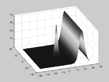
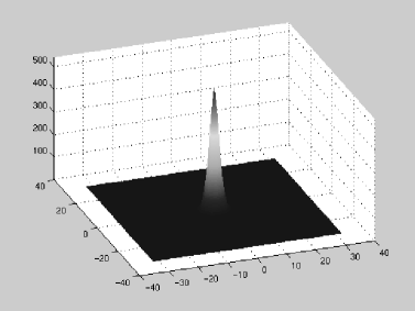
FIG. 1.: The first panel shows the potential energy density in the xz-plane for the magnetic monopole and domain wall where $h=-\lambda/5$, $\lambda=0.5$ and the wall velocity is $0.8c$. The second panel shows the corresponding magnetic energy density (proportional to ${B^{a}}_{i}^{2}$).

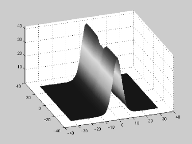
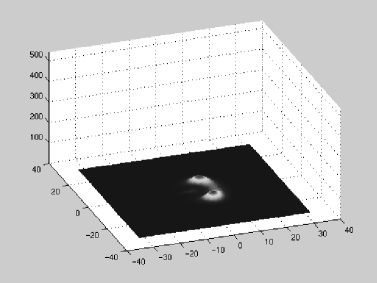
FIG. 2.: As in Fig. 1 at an intermediate time step.

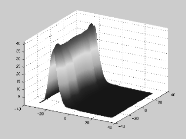
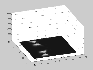
FIG. 3.: As in Fig. 1 at the final time step.

As is clear from Fig. 3, the final state of the wall is different from that of the initial wall. The destruction of the monopole has left a residue of scalar and magnetic excitations on the domain wall that are propagating along and behind the wall.

The dissolution of magnetic monopoles by domain walls implies that the number density of magnetic monopoles will fall off faster than if there were no domain walls. The cosmology of such a system of walls and monopoles has been discussed in [1] where it was argued that such interactions might resolve the cosmological monopole over-abundance problem. Similar interactions between strings and domain walls would affect the cosmological implications of cosmic strings. The numerical techniques presented here can also be used to study the interactions of walls and (global) monopoles or vortices in other systems.

We would like to thank Mark Meckes for providing the SU(5) BPS monopole solution, Ken Olum for numerical advice and especially Paul Saffin for bringing Ref. [10] to our attention. We thank the the National Energy Research Scientific Computing Center (NERSC) for the use of their J90 cluster on which some of the simulations were run. This work was supported by the Department of Energy (DOE).

REFERENCES

- [1] G. Dvali, H. Liu and T. Vachaspati, Phys. Rev. Lett. 80, 2281 (1998).
- [2] E. P. S. Shellard, Ph. D. Thesis, University of Cambridge (1986).
- [3] H.-R. Trebin and R. Kutka, J. Phys. A28, 2005 (1995); T. Sh. Misirpashaev, Sov. Phys. JETP 72, 973 (1991); M. Krusius, E.V. Thuneberg and U. Parts, Physica B197, 376 (1994).
- [4] A. E. Kudryavtsev, B. M. A. G. Piette and W. J. Zakrzewski, Nonlinearity 11, 783 (1998); hep-th/9907197.
- [5] S. Alexander, R. Brandenberger, R. Easther and A. Sornborger, hep-ph/9903254.
- [6] C. P. Dokos and T. N. Tomaras, Phys. Rev.D21, 2940 (1980).
- [7] E. B. Bogomolnyi, Sov. J. Nucl. Phys. 24, 449 (1976).
- [8] M. K. Prasad and C. M. Sommerfield, Phys. Rev. Lett. 35, 760 (1975).
- [9] M. Meckes, private communication (1999).
- [10] M. Alcubierre, S. Brandt, B. Brügmann, D. Holz, E. Seidel, R. Takahashi and J. Thornburg, gr-qc/9908012.