LPT–Orsay–99–68 SPbU–IP–99–12 hep-ph/9909539

Evolution equations for quark-gluon distributions in multi-color QCD and open spin chains

S.É. Derkachov¹, G.P. Korchemsky² and A.N. Manashov³

¹ Institut für Theoretische Physik, Universität Leipzig,
Augustusplatz 10, D-04109 Leipzig, Germany and
Department of Mathematics, St.-Petersburg Technology Institute,
St.-Petersburg, Russia

² Laboratoire de Physique Théorique, Université de Paris XI,
91405 Orsay Cédex, France

³ Department of Theoretical Physics, Sankt-Petersburg State University,
St.-Petersburg, Russia
Abstract:
We study the scale dependence of the twist-3 quark-gluon parton distributions using the observation that in the multi-color limit the corresponding QCD evolution equations possess an additional integral of motion and turn out to be effectively equivalent to the Schrödinger equation for integrable open Heisenberg spin chain model. We identify the integral of motion of the spin chain as a new quantum number that separates different components of the twist-3 parton distributions. Each component evolves independently and its scale dependence is governed by anomalous dimension given by the energy of the spin magnet. To find the spectrum of the QCD induced open Heisenberg spin magnet we develop the Bethe Ansatz technique based on the Baxter equation. The solutions to the Baxter equation are constructed using different asymptotic methods and their properties are studied in detail. We demonstrate that the obtained solutions provide a good qualitative description of the spectrum of the anomalous dimensions and reveal a number of interesting properties. We show that the few lowest anomalous dimensions are separated from the rest of the spectrum by a finite mass gap and estimate its value.

1. Introduction

The evolution equations play an important rôle in the QCD studies of hard processes as they allow to find the dependence of hadronic observables on the underlying high-energy scales [1]. It has been recognized recently that in different kinematical limits the QCD evolution equations possess an additional hidden symmetry. Namely, the Regge asymptotics of hadronic scattering amplitudes [2, 3] and the scale dependence of the leading twist light-cone baryonic distribution amplitudes [4] reveal remarkable properties of integrability. Both problems turn out to be intrinsically equivalent to the Heisenberg closed spin magnet which is known to be integrable $(1+1)-$dimensional quantum mechanical system and their solutions can be found by applying powerful methods of Integrable Models [5]. In the present paper we continue the study of integrable QCD evolution equations initiated in [4, 6] by considering the evolution equations for twist-three quark-gluon distribution functions. These functions describe the correlations between quarks and gluons in hadrons and provide an important information about the structure of hadronic states in QCD. They determine the twist-3 nucleon parton distributions [7] and the high Fock components of the meson wave functions [8] which in turn can be accessed experimentally through the measurement of different asymmetries.

The twist-3 quark-gluon distribution functions $D(x_{1},x_{2},x_{3};\mu)$ can be defined in QCD in terms of hadronic matrix elements of nonlocal gauge invariant light-cone operators ${\cal F}(z_{1},z_{2},z_{3})$ as [9]

$$\langle{p,s|{\cal F}(z_{1},z_{2},z_{3})|p,s}\rangle=\int_{-1}^{1}{\cal D}x\ \mbox{e}^{i(x_{1}z_{1}+x_{2}z_{2}+x_{3}z_{3})(pn)}{D}(x_{1},x_{2},x_{3};\mu)\,,$$ (1.1)

where ${\cal D}x=dx_{1}dx_{2}dx_{3}\delta(x_{1}+x_{2}+x_{3})$ and $|p,s\rangle$ is the nucleon state with momentum $p$ and spin $s$. The distribution function ${D}(x_{1},x_{2},x_{3};\mu)$ vanishes outside the region $-1<x_{1,2,3}<1$ and the scaling variables $x_{1}$, $x_{2}$ and $-x_{3}$ have a meaning of hadron momentum fractions carried by quark, gluon and antiquark, respectively, in the infinite momentum frame [9]. For $0<x_{i}<1$ (or $-1<x_{i}<0$) the corresponding parton belongs to the initial (or final) state nucleon. The matrix element entering the l.h.s. of (1.1) contains ultraviolet divergences that are subtracted at the scale $\mu$. The normalization scale $\mu$ defines the transverse separation of the partons and is determined by the hard scale of the underlying process [1].

The operator ${\cal F}(z_{1},z_{2},z_{3})$ describes the interacting system of quark, antiquark and gluon “living” on the light-front $y_{\mu}=zn_{\mu}$ with $n^{2}=0$ and separated along the $z-$direction. The twist-3 operator ${\cal F}(z_{1},z_{2},z_{3})$ is given by one of the following expressions [10, 11]

$$S^{\pm}_{\perp}(z_{1},z_{2},z_{3}) = \bar{q}(z_{1}n)\left[\widetilde{G}_{\perp\nu}(z_{2}n)\pm iG_{\perp\nu}(z_{2}n)\gamma_{5}\right]n^{\nu}{\not\!n}\,q(z_{3}n)$$ (1.2)

$$T_{\Gamma}(z_{1},z_{2},z_{3}) = \bar{q}(z_{1}n)n_{\mu}\sigma^{\mu\rho}n^{\nu}G_{\nu\rho}(z_{2}n)\Gamma\,q(z_{3}n)$$ (1.3)

with $\Gamma=\{\hbox{{1}\kern-2.5pt\hbox{l}}\,,i\gamma_{5}\}$, $\widetilde{G}_{\mu\nu}=\epsilon_{\mu\nu\rho\lambda}G^{\rho\lambda}/2$ being dual gluon field strength and “$\perp$” denoting the “transverse” Lorentz components orthogonal to the plane defined by the vectors $p_{\mu}$ and $n_{\mu}$. The definition of the chiral-even and chiral-odd quark-gluons distributions corresponding to the operators (1.2) and (1.3), respectively, and their relation to the twist-3 nucleon parton distributions are given in the Appendix A. In order to avoid additional complication due to mixing of the chiral-even operators $S^{\pm}$ with pure gluonic operators we will assume quarks to be of different (massless) flavor. It is implied that the gauge invariance of the operators (1.2) and (1.3) is restored by including non-Abelian phase factors $P\mbox{e}^{i\int dx^{\mu}A_{\mu}(x)}$ connecting gluon strength field with quark and antiquark fields.

In this paper we shall study the $\mu-$dependence of the distribution functions (1.1) in the multi-color QCD. The standard way of finding this dependence [10, 12, 13] consists in expanding nonlocal operator ${\cal F}(z_{1},z_{2},z_{3})$ entering (1.1) over the set of local gauge invariant composite operators ${\cal O}_{N,n}=\bar{q}(n\stackrel{{\scriptstyle\leftarrow}}{{D}})^{n}G(n\stackrel{{\scriptstyle\rightarrow}}{{D}})^{N-n}q$ with $n=0$, $...$, $N+1$ and $D_{\mu}=\partial_{\mu}-igA_{\mu}$ being the covariant derivative. In this way, one finds the evolution of the moments $\int_{-1}^{1}dx_{1}dx_{2}dx_{3}\delta(x_{1}+x_{2}+x_{3})\,x_{1}^{N-n}x_{3}^{n}\,{D}(x_{i})$ by diagonalizing a nontrivial $(N+1)\times(N+1)$ mixing matrix of the operators ${\cal O}_{N,n}$. It becomes straightforward to calculate numerically the spectrum of the anomalous dimensions for any given $N$ [13] but the general analytical structure of the spectrum remains unknown. To overcome this problem we apply the approach developed in [6]. It allows to construct the basis of local twist-3 quark-gluon operators which evolve independently and whose anomalous dimensions can be calculated analytically.

According to the definition, Eq. (1.1), the $\mu-$dependence of the twist-3 quark-gluon distributions follows from the renormalization group evolution of the corresponding nonlocal operators (1.2) and (1.3). To leading logarithmic accuracy one finds [11]

$$\frac{d}{d\ln\mu}{\cal F}(z_{1},z_{2},z_{3})=-\frac{\alpha_{s}N_{c}}{2\pi}{\cal H}_{\cal F}\cdot{\cal F}(z_{1},z_{2},z_{3})$$ (1.4)

with ${\cal H}_{\cal F}$ being some integral operator describing a pair-wise interaction between quark, gluon and antiquark with the light-cone coordinates $z_{1}$, $z_{2}$ and $z_{3}$, respectively. The approach of [6] is based on the identification of the evolution equation (1.4) as one-dimensional Schrödinger equation for three particles with a pair-wise interaction. The light-cone coordinates of the quarks and gluon $y_{i}^{\mu}=z_{i}n^{\mu}$ define the spacial coordinates, $z_{i}$, whereas the evolution parameter $\ln\mu^{2}$ plays the rôle of the evolution time. The integration of three-body Schrödinger equation (1.4) becomes problematic unless there exists an additional symmetry. It turns out that this is the case for the twist-3 quark-gluon correlation functions ${D}(x_{i};\mu)$. The corresponding evolution equation (1.4) possesses an additional “hidden” integral of motion in the multi-color limit and, as a consequence, it is completely integrable [4]. As we will show, the underlying integrable structure is identical to that for the integrable open noncompact $SL(2;\mathbb{R})$ spin chain models. Similar conclusions have been reached in the recent publications [14]. Our results partially overlap with the results of [4, 14] and we shall comment on their relation below.

“Noncompactness” of the spin group is a novel feature that QCD brings into the theory of integrable open spin magnets and that makes the analysis of the evolution equations interesting on its own. We would like to notice that an additional motivation for studying noncompact integrable open spin chains comes from the recent analysis of the Regge asymptotics of quark-gluon scattering amplitudes [15]. We also expect that these models (in their generalized version) will inevitably appear in the analysis of the evolution equations for higher twist quark-gluon correlation functions [7].

In the present paper we develop an approach for solving noncompact open spin chains models based on the Baxter equation and the fusion relations and apply it to find the spectrum of the anomalous dimensions of the twist-3 quark-gluon correlation functions in the leading logarithmic approximation in the multi-color QCD. As we will demonstrate this spectrum exhibits a number of interesting properties. The few lowest anomalous dimensions turn out to be separated from the rest of the spectrum by a finite “mass gap” and can be calculated exactly. The remaining part of the spectrum can be calculated using different asymptotic methods and the obtained approximate expression agree well with the exact results for large spin $N$.

The presentation is organized as follows. In Section 2 we explore the conformal symmetry of the evolution equations to write the QCD evolution kernels in the “normal” form in which their conformal invariance becomes manifest. In Section 3 we construct a general integrable open spin magnet and identify the values of parameters for which the Hamiltonian of the model coincides with the QCD evolution kernels for nonlocal operators $S^{\pm}_{\perp}$ and $T$. Section 4 is devoted to diagonalization of the conserved charge by means of the Algebraic Bethe Ansatz. Section 5 contains a derivation of the expression for the energy of the open spin magnet, or equivalently the spectrum of the anomalous dimensions of the quark-gluon correlation functions, in terms of the solutions to the Baxter equation. In Section 6 we study the properties of the Baxter equation and find its exact solutions. In Section 7 the asymptotic methods are applied to describe a fine structure of the spectrum. Summary of the main results is given in Section 8. In Appendix A the relation between the quark-gluon distributions and twist-3 nucleon structure functions is discussed. Appendix B contains definition and some properties of the Wilson polynomials.

2. QCD evolution kernels

In the multi-color limit the QCD evolution kernel ${\cal H}_{\cal F}$ entering (1.4) gets contribution only from planar diagrams and to one-loop level it is equal to the sum of the quark-gluon and antiquark-gluon interaction kernels while the interaction between quark and antiquark is suppressed by a color factor $1/N_{c}^{2}$. The kernel ${\cal H}_{\cal F}$ depends on the choice of nonlocal operator and for twist-3 nonlocal operators defined in (1.2) and (1.3) it is given in the multi-color limit by the following expressions [4]

$${\cal H}_{T}=\psi\left(J_{qg}+\frac{3}{2}\right)+\psi\left(J_{qg}-\frac{3}{2}\right)+\psi\left(J_{g\bar{q}}+\frac{3}{2}\right)+\psi\left(J_{g\bar{q}}-\frac{3}{2}\right)+\delta$$ (2.1)

$${\cal H}_{S^{+}}=\psi\left(J_{qg}+\frac{3}{2}\right)+\psi\left(J_{qg}-\frac{3}{2}\right)+\psi\left(J_{g\bar{q}}+\frac{1}{2}\right)+\psi\left(J_{g\bar{q}}-\frac{1}{2}\right)+\delta$$ (2.2)

with $\psi(x)=d\ln\Gamma(x)/dx$, $\delta=-3/2+4\gamma_{{}_{\rm E}}$ and $J_{ik}$ being the operators acting on the light-cone coordinates of the partons $(i,k=q,g,\bar{q})$ and defined below in (2.5). Here, the kernel ${\cal H}_{T}$ governs the RG evolution of the operators $T_{\Gamma}(z_{i})$. To one-loop level it does not depend on the choice of $\Gamma$ and we will not indicate the subscript $\Gamma$ explicitly. The kernel ${\cal H}_{S^{-}}$ is obtained from ${\cal H}_{S^{+}}$ by interchanging the coordinates of quark and antiquark and therefore it will not be considered separately.

It is well known [16] that to one-loop level the QCD evolution kernels (2.1) and (2.2) inherit the conformal symmetry of the bare QCD Lagrangian which is reduced on the light-cone to its $SL(2,\mathbb{R})$ subgroup generating a projective transformation $z\to(az+b)/(cz+d)$ on the line $y_{\mu}=zn_{\mu}$ with $ad-bc=1$. Denoting the $SL(2,\mathbb{R})$ generators as $L_{+}$, $L_{-}$ and $L_{0}$ we define their action on the quark and gluon fields $\Phi(z)\equiv\left\{\bar{q}(nz),\,q(nz),\,n^{\mu}G_{\mu\nu}(nz)\right\}$ on the light-cone $n^{2}_{\mu}=0$ as

$$L_{-,{k}}\Phi(z_{k}) = -\partial_{z_{k}}\Phi(z_{k})$$

$$L_{+,{k}}\Phi(z_{k}) = \left(z^{2}_{k}\partial_{z_{k}}+2j_{k}z_{k}\right)\Phi(z_{k})$$ (2.3)

$$L_{0,{k}}\Phi(z_{k}) = \left(z_{k}\partial_{z_{k}}+j_{k}\right)\Phi(z_{k})\,,$$

where $j_{k}=(l_{k}+s_{k})/2$ is the conformal spin of the field $\Phi_{k}$ (${k}=\bar{q},q,g$) defined as the sum of its canonical dimension, $l_{k}$, and the projection of its spin on the line $zn^{\mu}$, $\Sigma_{+-}\Phi_{k}=is_{k}\Phi_{k}$. In particular, using $l_{\bar{q}}=l_{q}=3/2$, $l_{g}=2$ together with $s_{\bar{q}}=s_{q}=1/2$, $s_{g}=1$ we get the conformal spins as

$$j_{\bar{q}}=j_{q}=1\,,\qquad j_{g}=3/2$$ (2.4)

for (anti-)quark and gluon fields, respectively.

The operators $J_{qg}$ and $J_{\bar{q}g}$ entering (2.2) and (2.1) are defined in terms of two-particle Casimir operators as follows

$$L_{ik}^{2}=J_{ik}(J_{ik}-1)\,,\qquad L_{ik,\alpha}=L_{i,\alpha}+L_{k,\alpha}$$ (2.5)

with $i,k=q\,,g\,,\bar{q}$ and $\alpha=0,\pm$. The eigenvalues of the operator $J_{qg}$ give the possible values of the spin in the quark-gluon channel and have the form $j_{qg}=j_{q}+j_{g}+n=5/2+n$ with $n$ being a nonnegative integer. The operator $J_{g\bar{q}}$ has a similar interpretation in the gluon-antiquark channel. The $SL(2)$ symmetry of the evolution kernels (2.1) and (2.2) becomes manifest

$$[{\cal H}_{\cal F},L_{\alpha}]=[{\cal H}_{\cal F},L^{2}]=[L_{\alpha},L^{2}]=0\,,$$ (2.6)

where $L_{\alpha}$ ($\alpha=\pm,\,0$) are the total three-particle $SL(2)$ generators

$$L_{\alpha}=L_{\alpha,\bar{q}}+L_{\alpha,q}+L_{\alpha,g}\,,\qquad L^{2}=\frac{1}{2}\left(L_{+}L_{-}+L_{-}L_{+}\right)+L_{0}^{2}\,.$$ (2.7)

Note that the conformal invariance holds separately for all terms entering the $1/N_{c}-$expansion of the evolution kernels (2.2) and (2.1).

Going from the matrix element of nonlocal operator to the quark-gluon distribution function, Eq. (1.1), we find that $D(x_{1},x_{2},x_{3})$ obeys the RG equation similar to (1.4) with the Hamiltonian ${\cal H}_{\cal F}$ transformed from the coordinate $z-$representation into the momentum $x-$representation. The analysis of the evolution equation for $D(x_{1},x_{2},x_{3})$ is based on the solutions to the Schrödinger equation [6]

$${\cal H}_{\cal F}\cdot\Psi_{N,q}(x_{1},x_{2},x_{3})={\cal E}_{N,q}\Psi_{N,q}(x_{1},x_{2},x_{3})\,,$$ (2.8)

where the eigenstates $\Psi_{N,q}(x_{i})$ are homogeneous polynomials in $x_{i}$ of degree $N$ and index $q$ enumerates different energy levels ${\cal E}_{N,q}$. Here, the Hamiltonian is given by the evolution kernels (2.1) and (2.2) with the $SL(2;\mathbb{R})$ generators defined in the $x-$representation as

$$L_{k,0}\Psi(x_{i}) = (x_{k}\partial_{k}+j_{k})\Psi(x_{k})$$

$$L_{k,+}\Psi(x_{i}) = -x_{k}\Psi(x_{k})$$ (2.9)

$$L_{k,-}\Psi(x_{i}) = (x_{k}\partial_{x_{k}}^{2}+2j_{k}\partial_{x_{k}})\Psi(x_{k})\,.$$

Finally, solving the Schrödinger equation (2.8) one can construct the basis of local conformal operators [6]

$${\cal O}_{N,q}(0)=\Psi_{N,q}(i\partial_{z_{1}},i\partial_{z_{2}},i\partial_{z_{3}}){\cal F}(z_{1},z_{2},z_{3})\bigg{|}_{z_{i}=0}\,,$$ (2.10)

which have a fixed operator dimension, or equivalently a fixed total number $N$ of covariant derivatives, and which do not mix under renormalization. It follows from (2.8) that their anomalous dimensions are determined by the energy of the state $\Psi_{N,q}$

$$\gamma_{q}(N)=\frac{\alpha_{s}N_{c}}{2\pi}{\cal E}_{N,q}$$ (2.11)

while their matrix elements over nucleon states evaluated at a low normalization scale $\mu_{0}$ define the set of nonperturbative dimensionless parameters

$$\phi_{N,q}(\mu_{0})=\langle{p,s|{\cal O}_{N,q}(0)|p,s}\rangle_{\mu=\mu_{0}}\,.$$ (2.12)

Substituting (1.1) into (2.10) one finds the solution to the evolution equation for (generalized) moments of the distribution functions as

$$\int_{-1}^{1}{\cal D}x\,\Psi_{N,q}(x_{1},x_{2},x_{3}){D}(x_{1},x_{2},x_{3})=\phi_{N,q}(\mu_{0})\left(\frac{\alpha_{s}(\mu)}{\alpha_{s}(\mu_{0})}\right)^{{\cal E}_{N,q}/b_{0}}\,,$$ (2.13)

where $b_{0}=11N_{c}/3-2n_{f}/3$ and ${\cal D}x=dx_{1}dx_{2}dx_{3}\delta(x_{1}+x_{2}+x_{3})$. Inverting this relation one can obtain the expression for the distribution function as an integral over complex moments $N$.

Thus, the scale dependence of the twist-3 quark gluon distributions becomes effectively equivalent to the eigenproblem (2.8). In what follows we shall solve exactly the Schrödinger equation (2.8) and study in detail the properties of its solutions. Analyzing (2.8) one has to identify the total set of the conserved charges. The conformal symmetry allows to identify the degree $N$ of the polynomials $\Psi_{N,q}(x_{i})$ as a trivial integral of motion. For fixed $N$ the eigenstates $\Psi_{N,q}(x_{i})$ belong to the irreducible representation of the $SL(2,\mathbb{R})$ group parameterized by a total conformal spin $h=N+j_{\bar{q}}+j_{q}+j_{g}$ and satisfy the relations

$$L_{0}\Psi_{h}(x_{i}) = h\,\Psi_{h}(x_{i})\,,\quad h=N+\frac{7}{2}$$

$$L_{-}\Psi_{h}(x_{i}) = 0$$ (2.14)

$$L^{2}\Psi_{h}(x_{i}) = h(h-1)\Psi_{h}(x_{i})\,.$$

Thus defined $\Psi_{h}(x_{i})$ can be identified as the highest weights of the $SL(2,\mathbb{R})$ representations labeled by a nonnegative integer $N$. Note that for given $\Psi_{h}(x_{i})$ there exists an infinite series of the “excited” eigenstates, $(L_{+})^{m}\Psi_{h}=(-x_{1}-x_{2}-x_{3})^{m}\Psi_{h}$, which vanish due to $x_{1}+x_{2}+x_{3}=0$.

However the conformal symmetry does not fix the eigenfunctions $\Psi_{h}(x_{i})$ uniquely. This can be seen in a number of ways. According to (2.7) the total conformal spin $h$ is equal to the sum of the conformal spin of the quark-gluon system and the conformal spin of antiquark. For given $h$ the value of the spin in the $qg-$channel can be arbitrary, $j_{qg}=j_{q}+j_{g}+m=5/2+m$ with $0\leq m\leq N$, and this leads to an additional degeneracy in solutions to (2.14). The degeneracy can be removed if there exists one more $SL(2)$ invariant conserved charge $Q$. In this case, the Schrödinger equation (2.8) becomes completely integrable – the number of degrees of freedom matches the number of the conserved charges, $L_{0}$, $L^{2}$ and $Q$, and, as a consequence, the wave functions, $\Psi_{N,q}$, and the energy, ${\cal E}_{N,q}$, are uniquely fixed by the conformal spin $N$ and the eigenvalues, $q$, of the charge $Q$.

It turns out that such operator exists for the evolution kernels corresponding to the twist-3 quark-gluon operators in the multi-color limit, Eqs. (2.1) and (2.2)

$$[{\cal H}_{S^{\pm}},Q_{S^{\pm}}]=0\,,\qquad[{\cal H}_{T},Q_{T}]=0\,.$$ (2.15)

The $SL(2)$ invariant charges $Q_{S^{+}}$ and $Q_{T}$ are given by [4]

$$Q_{S^{+}} = \{L_{12}^{2},L_{23}^{2}\}-\frac{1}{2}L_{12}^{2}-\frac{9}{2}L_{23}^{2}$$ (2.16)

$$Q_{T} = \{L_{12}^{2},L_{23}^{2}\}-\frac{9}{2}L_{12}^{2}-\frac{9}{2}L_{23}^{2}\,,$$ (2.17)

where $\{\,,\}$ stands for an anticommutator, $L_{12}^{2}\equiv L_{qg}^{2}$ and $L_{23}^{2}\equiv L_{g\bar{q}}^{2}$ are two-particle Casimir operators in the quark-gluon and gluon-antiquark channels. The charge $Q_{S^{-}}$ is obtained from $Q_{S^{+}}$ by permutation of the particles $(123)\to(321)$. The kernel ${\cal H}_{T}$ is invariant under this transformation and, as a consequence, its eigenstates have a definite parity under $z_{1}\leftrightarrow z_{3}$.

3. Integrability of the effective QCD Hamiltonian

Let us demonstrate that the Schrödinger equation (2.8) defined by the evolution kernels Eqs. (2.1) and (2.2) is equivalent in the multi-color limit to the one-dimensional Heisenberg open spin chain model. To this end, we shall apply the Quantum Inverse Scattering Method [5, 17] to construct an integrable (inhomogeneous) open spin chain model and show that for certain values of parameters the Hamiltonian of this model coincides with the QCD evolution kernels (2.1) and (2.2).

3.1. Open spin chains

To start with we consider $M$ particles with the coordinates $x_{n}$ $(n=1,...,M)$ on a line and assign to each particle three $SL(2)$ generators $(L_{+,n},L_{-,n},L_{0,n})$. In what follows we shall refer to these generators as to spin$-j_{n}$ operators. They are realized as differential operators (2.3) acting on the quantum space of the $n-$th particle that we denote as $V_{j_{n}}$. The interaction between $M$ particles occurs through a pair-wise interaction between the nearest-neighbor spins. The corresponding pair-wise Hamiltonians depend on the two-particle Casimir operators $L_{jk}^{2}$

$$L_{jk}^{2}=\sum_{\alpha=0,1,2}(L_{\alpha,j}+L_{\alpha,k})^{2}\,,\qquad j\,,k=1\,,...\,,M$$ (3.1)

with $L_{\pm,j}\equiv L_{1,j}\pm iL_{2,j}$.

The definition of the model is based on the existence of the solution to the Yang-Baxter equation

$$R_{j_{1}j_{2}}(u)R_{j_{1}j_{3}}(v)R_{j_{2}j_{3}}(u-v)=R_{j_{2}j_{3}}(u-v)R_{j_{1}j_{3}}(v)R_{j_{1}j_{2}}(u)\,.$$ (3.2)

Here, the operator $R_{j_{1}j_{2}}(u)$ acts on the tensor product of the quantum spaces $V_{j_{1}}\otimes V_{j_{2}}$ and depends on an arbitrary complex spectral parameter $u$. The solution to (3.2) is given by [18, 19]

$$R_{j_{1}j_{2}}(u)=(-)^{J_{12}+j_{1}+j_{2}}\frac{\Gamma(J_{12}-iu)}{\Gamma(J_{12}+iu)}\frac{\Gamma(j_{1}+j_{2}+iu)}{\Gamma(j_{1}+j_{2}-iu)}\,,$$ (3.3)

where the operator $J_{12}$ is given by the sum of two $SL(2)$ spins and it is defined as a formal solution to

$$J_{12}(J_{12}-1)=L_{12}^{2}\,.$$ (3.4)

For arbitrary $SL(2)$ spins $j_{1}$ and $j_{2}$ the eigenvalues of the operator $J_{12}$ have the form $j_{12}=j_{1}+j_{2}+n$ with $n=0\,,1\,,...$, which correspond to decomposition of the tensor product $V_{j_{1}}\otimes V_{j_{2}}$ over the irreducible $SL(2)$ components of spin $j_{12}$.

Having the explicit expression for the $R-$operator, Eq.(3.3), we construct an integrable open spin model following Sklyanin [17]. Namely, we define the monodromy operator acting on the space $V_{j}\otimes V_{j_{1}}\otimes...\otimes V_{j_{M}}$

$$T_{j}(u)=R_{j_{1}j}(u-i\omega_{1})R_{j_{2}j}(u-i\omega_{2})...R_{j_{M}j}(u-i\omega_{M})$$ (3.5)

with $j$ being the spin of the auxiliary space $V_{j}$ and $\omega_{k}$ being the shifts (spin chain impurities) associated with the $k-$th particle. Let us impose the additional condition that the spins and the impurities of all “intermediate” sites are the same

$$j_{2}=j_{3}=...=j_{M-1}\,,\qquad\omega_{2}=\omega_{3}=...=\omega_{M-1}\,,$$ (3.6)

while $j_{2}\neq j_{1},j_{M}$ and $\omega_{2}\neq\omega_{1},\omega_{M}$.

As we will show in Sect. 3.2 it is this condition (together with $\omega_{2}=0$ and $M=3$) that one finds matching the QCD evolution kernels, (2.1) and (2.2), into integrable spin chain Hamiltonian. Then, the transfer matrix of the open spin chain with $M$ sites is defined as

$$t_{j}(u)=\mbox{tr}_{j}\left[T_{j}(u)T^{-1}_{j}(-u)\right]\,.$$ (3.7)

Here, the trace is taken over the auxiliary $SL(2)$ representation space of the spin $j$. Choosing different values of $j$ one obtains (an infinite) set of the transfer matrices $t_{j}(u)$ which by virtue of the Yang-Baxter equation (3.2) commute with each other for different values of the spectral parameters

$$[t_{j_{1}}(u),t_{j_{2}}(v)]=0$$ (3.8)

for any $j_{1}$ and $j_{2}$. As a consequence, expanding $t_{j}(u)$ in powers of the spectral parameter $u$ and choosing different values of the spin $j$ one obtains the family of mutually commuting operators. Their explicit form depends on the set of parameters, $j_{k}$ and $\omega_{k}$, which define the spectrum of spins and impurities of the model, respectively. This family contains the Hamiltonian ${\cal H}_{M}$ of the model as well as a complete set of the conserved charges. In addition, the transfer matrix possesses an additional $SL(2)$ symmetry

$$[t_{j}(u),L_{\alpha}]=0\,,\qquad L_{\alpha}=L_{\alpha,1}+...+L_{\alpha,M}\,,\quad\alpha=0\,,\pm\,,$$ (3.9)

which ensures the $SL(2)$ invariance of the Hamiltonian, (2.6).

3.2. Integrals of motion

Let us show that the QCD integrals of motion (2.17) and (2.16) appear in the expansion of the spin$-1/2$ transfer matrix, $t_{-1/2}(u)$, given by (3.7) with the auxiliary $SL(2)$ spin $j=-1/2$ and the number of sites $M=3$.

It is well known [22, 5], that the spin$-1/2$ $R-$operator (3.3) coincides with the Lax operator of the Heisenberg spin chain, $R_{-\frac{1}{2}j_{k}}(u)\equiv{\mathbb{L}}_{j_{k}}(u)$

$${\mathbb{L}}_{j}(u)=u+\frac{i}{2}-i\sum_{\alpha=0,\pm}L_{\alpha}\,\sigma^{\alpha}=\left(\begin{array}[]{cc}u+\frac{i}{2}-iL^{3}&-iL^{-}\\ -iL^{+}&u+\frac{i}{2}+iL^{3}\end{array}\right)$$ (3.10)

with $L_{\alpha}$ being spin$-j$ generators and $L_{\pm}=L_{1}\pm iL_{2}$. Substituting (3.10) into (3.5) one evaluates the spin$-1/2$ monodromy operator as a $2\times 2$ matrix

$$T_{-1/2}(u)={\mathbb{L}}_{j_{1}}(u-i\omega_{1})...{\mathbb{L}}_{j_{M}}(u-i\omega_{M})=\left(\begin{array}[]{cc}a(u)&b(u)\\ c(u)&d(u)\end{array}\right)\,.$$ (3.11)

Here, $a(u)$, $b(u)$, $c(u)$ and $d(u)$ are expressed in terms of the spin operators and satisfy the Yang-Baxter relations of the form

$$[b(u),c(v)]=i\frac{d(v)a(u)-a(v)d(u)}{u-v}$$ (3.12)

together with similar relations for other components of $T_{-1/2}(u)$. The spin$-1/2$ transfer matrix $t_{-1/2}(u)$ is given by (3.7) with $T_{-1/2}(u)$ replaced by its expression (3.11). It proves convenient to change the normalization of the transfer matrix by introducing the following operator [17]

$$\widehat{t}_{-1/2}(u)=t_{-1/2}\left(-u-\frac{i}{2}\right)\rho(u)\,,$$ (3.13)

where the c-valued factor $\rho(u)$ compensates the poles of $t_{-1/2}(-u-i/2)$ and is given by

$$\rho(u)=\prod_{k=1}^{M}(u+ij_{k}^{-})(u-ij_{k}^{+}+i)$$ (3.14)

with the parameters $j_{k}^{\pm}$ defined as

$$j_{k}^{\pm}=j_{k}\pm\omega_{k}\,.$$ (3.15)

Thus defined normalized transfer matrix can be expressed as [17]

$$\widehat{t}_{-1/2}(u)=\mbox{tr}\,\widehat{T}_{-1/2}(u)\,,\qquad\widehat{T}_{-1/2}(u)=T_{-1/2}{\left({u-\frac{i}{2}}\right)}\,\sigma_{2}\,T_{-1/2}^{t}{\left({-u-\frac{i}{2}}\right)}\,\sigma_{2}$$ (3.16)

and it has the following properties. Firstly, in contrast with $t_{-1/2}(u)$, the normalized transfer matrix does not have poles in $u$ and, secondly, $\widehat{t}_{-1/2}(u)$ has the form of a polynomial of degree $M$ in $u^{2}$ with the corresponding operator coefficients providing the set of the conserved charges of the model.

It becomes straightforward to calculate the normalized transfer matrix $\widehat{t}_{-1/2}(u)$ for the chain with $M=3$ sites. Substituting (3.10) into (3.11) and (3.16) one finds after some algebra

$$\widehat{t}_{-1/2}(u)=(4u^{2}+1)\tau(u^{2})-2\prod_{k=1,2,3}\left(u^{2}-L_{k}^{2}+\omega_{k}^{2}\right)$$ (3.17)

with one-particle Casimir operators $L_{k}^{2}=j_{k}(j_{k}-1)$ being c-numbers and the operator $\tau(u^{2})$ defined as

$$\tau(u^{2}) = u^{2}[L^{2}-\sum_{k=1,2,3}L_{k}^{2}]+L^{2}\left[L_{2}^{2}+\omega_{2}^{2}\right]-\frac{1}{2}Q$$ (3.18)

$$+L_{1}^{2}L_{3}^{2}-L_{1}^{2}\omega_{3}^{2}-L_{2}^{2}(\omega_{1}^{2}-\omega_{2}^{2}+\omega_{3}^{2})-L_{3}^{2}\omega_{1}^{2}\,.$$

The charge $Q$ is given by

$$Q=-2{\omega_{2}}\ [L_{12}^{2},L_{23}^{2}]_{-}+\{L_{12}^{2},L_{23}^{2}\}_{+}+2(\omega_{2}^{2}-\omega_{3}^{2})\ L_{12}^{2}+2(\omega_{2}^{2}-\omega_{1}^{2})\ L_{23}^{2}\,.$$ (3.19)

with $L_{jk}^{2}$ and $L^{2}$ being two- and three-particle Casimir operators defined in (3.1) and (2.7), respectively.

The normalized transfer matrix (3.17) involves two mutually commuting operators, $Q$ and $L^{2}$. Together with $L_{0}$ they form the complete set of the conserved charges for integrable open chain of $M=3$ particles with arbitrary values of the spins $j_{k}$ and the impurity parameters $\omega_{k}$. To fix their values we compare (3.19) with the expressions for the integrals of motion of the QCD evolution equations, Eqs. (2.17) and (2.16). We find that the spins of particles are equal to the conformal spins of the corresponding fields

$$j_{1}=j_{3}=1\,,\qquad j_{2}=\frac{3}{2}\,,$$ (3.20)

and the impurity parameters are given by

$$Q_{S^{+}}:\qquad\omega_{1}^{2}=\frac{9}{4}\,,\quad\omega_{2}=0\,,\quad\omega_{3}^{2}=\frac{1}{4}$$ (3.21)

and

$$Q_{T}\ :\qquad\omega_{1}^{2}=\frac{9}{4}\,,\quad\omega_{2}=0\,,\quad\omega_{3}^{2}=\frac{9}{4}\,.$$ (3.22)

These matching conditions define the parameters $\omega_{1}$ and $\omega_{3}$ up to a sign. As we will show in Sect. 3.3, the Hamiltonian of the model is invariant under $\omega_{1,3}\to-\omega_{1,3}$.

Eqs. (3.20), (3.21) and (3.22) establish the equivalence relations between the QCD evolution kernels and the open spin chain models. Instead of considering two cases (3.21) and (3.22) separately, we shall treat $\omega_{1}$ and $\omega_{3}$ as free parameters and introduce the charge

$$Q(\omega_{1},\omega_{3})=\{L_{12}^{2},L_{23}^{2}\}_{+}-2\omega_{3}^{2}\ L_{12}^{2}-2\omega_{1}^{2}\ L_{23}^{2}\,.$$ (3.23)

In what follows we shall find the flow of the eigenvalues of this charge, $q(\omega_{1},\omega_{3})$, in the parameters $\omega_{1,3}$ and identify the integrals of motion, $q_{T}$ and $q_{S^{+}}$, as corresponding to the special values of the flow parameters

$$q_{S^{+}}=q\left(\frac{3}{2},\frac{1}{2}\right)\,,\qquad q_{T}=q\left(\frac{3}{2},\frac{3}{2}\right)\,.$$ (3.24)

3.3. Integrable Hamiltonian

Let us complete an identification of the QCD evolution equations as integrable systems by showing that the evolution kernels (2.1) and (2.2) coincide with the Hamiltonian of open spin chain model. The latter enters into the expansion of the transfer matrix $t_{j}(u)$ given by (3.7) with the auxiliary spin $j$ equal to the spin of intermediate “gluonic” site $j=j_{2}=3/2$. The corresponding monodromy operator takes the form

$$T_{j}(u)=R_{j_{1}j}(u-i\omega_{1})R_{j_{2}j}(u)R_{j_{3}j}(u-i\omega_{3})\bigg{|}_{j=j_{2}}\,,$$ (3.25)

where $\omega_{2}=0$, $j_{1}=j_{3}=1$ and $j_{2}=3/2$.

We would like to stress that the spin chain described by (3.25) is inhomogeneous - the spins and impurities of the end-points are different from the ones of the internal sites of the chain. To our best knowledge such QCD induced spin magnets have not been studied before and their analysis represents a certain interest from point of view of integrable models. It is for this reason that we generalize the definition (3.25) by enlarging the size of the open spin chain to an arbitrary number of sites, $M\geq 3$, and fixing the parameters (spins and impurities) according to (3.6)

$$T_{j}(u)=R_{j_{1}j}(u-i\omega_{1})R_{j_{2}j}(u)...R_{j_{M-1}j}(u)R_{j_{M}j}(u-i\omega_{M})\bigg{|}_{j=j_{2}=...=j_{M-1}}\,,$$ (3.26)

where we put $\omega_{2}=...=\omega_{M-1}=0$ in order to match (3.25) for $M=3$.

Finally, one finds the transfer matrix $t_{j}(u)$ by substituting the monodromy operator (3.26) into (3.7) and defines the Hamiltonian of inhomogeneous spin chain with $M$ sites as

$${\cal H}_{M}=\frac{i}{2}\partial_{u}\ln t_{j}(u=0)=\frac{i}{2}\partial_{u}\ln\mbox{tr}\left[T_{j}(u)T_{j}^{-1}(-u)\right]\bigg{|}_{u=0}\,.$$ (3.27)

We would like to notice that this relation differs from the standard definition of Hamiltonian based on the so-called fundamental monodromy operator [17, 22]. In contrast with the latter, the spins of quantum spaces $V_{j_{1}}$ and $V_{j_{M}}$ corresponding to the end-points of the chain (3.26) are different from that of the auxiliary space $V_{j}$.

One finds the explicit form of the Hamiltonian (3.27) in the standard way [17] by replacing the monodromy operator $T_{j}(u)$ by its expression (3.26) and taking into account the following property of the $R-$operator (3.3)

$$R_{j_{k}j}(0)={\mathbb{P}}_{j_{k}j}\,,\qquad k=2,...,M-1\,,$$ (3.28)

where ${\mathbb{P}}_{j_{2}j}$ is the permutation operator acting on the tensor product of the quantum spaces as ${\mathbb{P}}_{j_{2}j}[V_{j_{2}}\otimes V_{j}]=V_{j}\otimes V_{j_{2}}$ [18, 19]. Note that (3.28) holds only for intermediate sites with $j_{k}=j$ while the operators $R_{j_{1}j}$ and $R_{j_{M}j}$ corresponding to the end-points of the chain do not possess such property. As a consequence, the calculation of the Hamiltonian (3.27) deviates the standard derivation [17] and requires a special consideration.

Substituting (3.25) into (3.7) and (3.27) and making use of (3.28) we obtain after some algebra

$${\cal H}_{M}=H_{j_{1}j_{2}}(\omega_{1})+\sum_{k=2}^{M-2}H_{j_{k}j_{k+1}}(0)+H_{j_{M-1}j_{M}}(\omega_{M})+\Delta{\cal H}\,,$$ (3.29)

where the notation was introduced for the pair-wise Hamiltonian

$$H_{j_{k}j_{k+1}}(\omega)=-\partial_{\omega}R_{j_{k}j_{k+1}}(-i\omega)R_{j_{k}j_{k+1}}^{-1}(-i\omega)=-\partial_{\omega}R_{j_{k}j_{k+1}}(-i\omega)R_{j_{k}j_{k+1}}(i\omega)$$ (3.30)

and the operator $\Delta{\cal H}$ is defined as

$$\Delta{\cal H}=\mbox{tr}_{j}\left\{H_{j_{1}j}(\omega_{1})+R_{j_{1}j}(-i\omega_{1})H_{j_{2}j}(0)R_{j_{1}j}(i\omega_{1})-H_{j_{1}j_{2}}(\omega_{1})\right\}/\mbox{tr}_{j}\hbox{{1}\kern-2.5pt\hbox{l}}\,.$$ (3.31)

In comparison with the definition of the homogeneous spin chain Hamiltonian [17], the expression (3.29) contains the additional operator $\Delta{\cal H}$. One can show however that $\Delta{\cal H}$ provides a c-number correction to ${\cal H}_{M}$. To this end one differentiates the both sides of the Yang-Baxter equation

$$R_{jj_{1}}(u-i\omega_{1})R_{j_{2}j}(u)R_{j_{2}j_{1}}(-i\omega_{1})=R_{j_{2}j_{1}}(-i\omega_{1})R_{j_{2}j}(u)R_{jj_{1}}(u-i\omega_{1})$$

with respect to the spectral parameter $u$ and puts $u=0$. Then, multiplying the both sides of the relation from the right by ${\mathbb{P}}_{j_{2}j}$ and using (3.28) one arrives at

$$H_{jj_{1}}(\omega_{1})+R_{jj_{1}}(-i\omega_{1})H_{j_{2}j}(0)R_{jj_{1}}(i\omega_{1})=H_{j_{2}j_{1}}(\omega_{1})+R_{j_{2}j_{1}}(\omega_{1})H_{j_{2}j}(0)R_{j_{2}j_{1}}(-i\omega_{1})\,.$$ (3.32)

Using this identity one evaluates (3.31) as

$$\Delta{\cal H}=R_{j_{1}j_{2}}(i\omega_{1})\frac{\mbox{tr}_{j}H_{j_{2}j}(0)}{\mbox{tr}_{j}\hbox{{1}\kern-2.5pt\hbox{l}}}R_{j_{1}j_{2}}(-i\omega_{1})=\frac{\mbox{tr}_{j}H_{j_{2}j}(0)}{\mbox{tr}_{j}\hbox{{1}\kern-2.5pt\hbox{l}}}={\rm const}\times\hbox{{1}\kern-2.5pt\hbox{l}}_{j_{2}}\,.$$ (3.33)

In what follows we shall neglect the additive correction due to $\Delta{\cal H}$.

Thus, the integrable Hamiltonian of the inhomogeneous open spin chain with $M$ sites is given by (3.29) with the pair-wise Hamiltonian defined by (3.30) and (3.3) as

$$H_{j_{1}j_{2}}(\omega)=\psi(j_{12}-\omega)+\psi(j_{12}+\omega)-\psi(j_{1}+j_{2}-\omega)-\psi(j_{1}+j_{2}+\omega)$$ (3.34)

with $\psi(x)=d\ln\Gamma(x)/dx$ and the operator $j_{12}$ introduced in (3.4). This expression is valid for arbitrary spins $j_{1}$, $j_{2}$ and, as it was anticipated, it is an even function of the impurity parameter $\omega$.

It is now straightforward to see that for $M=3$ and the parameters $j_{k}$ and $\omega_{k}$ given by (3.20), (3.21) and (3.22), the Hamiltonian (3.29) coincides (up to an overall normalization) with the QCD evolution kernels (2.1) and (2.2). Following (3.23) we introduce the interpolating Hamiltonian depending on the flow parameters $\omega_{1,3}$

$${\cal H}(\omega_{1},\omega_{3}) = \psi(j_{12}-\omega_{1})+\psi(j_{12}+\omega_{1})-\psi(\mbox{$\frac{5}{2}$}-\omega_{1})-\psi(\mbox{$\frac{5}{2}$}+\omega_{1})$$ (3.35)

$$+ \psi(j_{23}-\omega_{3})+\psi(j_{23}+\omega_{3})-\psi(\mbox{$\frac{5}{2}$}-\omega_{3})-\psi(\mbox{$\frac{5}{2}$}+\omega_{3})\,.$$

Then, the relation between ${\cal H}(\omega_{1},\omega_{3})$ and the QCD evolution kernels, Eqs. (2.1) and (2.2), looks like

$${\cal H}_{S^{+}}={\cal H}\left(\frac{3}{2},\frac{1}{2}\right)+\frac{17}{6}\,,\qquad{\cal H}_{T}={\cal H}\left(\frac{3}{2},\frac{3}{2}\right)+\frac{13}{6}\,.$$ (3.36)

Thus, the energies ${\cal E}_{S^{\pm}}$ and ${\cal E}_{T}$ entering into the solutions to the QCD evolution equations (2.13) for the twist-3 quark-gluon distributions, $D_{S^{\pm}}(x_{i})$ and $D_{T}(x_{i})$, respectively, can be calculated as

$${\cal E}_{S^{+}}={\cal E}\left(\frac{3}{2},\frac{1}{2}\right)+\frac{17}{6}+{\cal O}(1/N_{c}^{2})\,,\qquad{\cal E}_{T}={\cal E}\left(\frac{3}{2},\frac{3}{2}\right)+\frac{13}{6}+{\cal O}(1/N_{c}^{2})\,,$$ (3.37)

where ${\cal E}(\omega_{1},\omega_{3})$ are eigenvalues of the Hamiltonian (3.35) and $1/N_{c}^{2}-$corrections correspond to nonplanar part of the evolution kernels (2.1) and (2.2).

Having identified the QCD evolution kernels (2.1) and (2.2) as Hamiltonians of the open spin chain model we now turn to the eigenvalue problem for (3.29). The complete integrability of the Hamiltonian (3.29) implies that ${\cal H}_{M}$ is a (complicated) function of the conserved charges. Using this dependence to which we shall refer as to the dispersion curve we can find the spectrum of the Hamiltonian by replacing the charges by their corresponding eigenvalues. However, instead of considering separately the eigenproblem for ${\cal H}_{M}$ we shall solve a more general problem of diagonalization the transfer matrices $t_{j}(u)$ of different spins $j$.

We recall that the conserved charges and the Hamiltonian are generated by two different transfer matrices, $t_{-1/2}(u)$ and $t_{j_{2}}(u)$, respectively. As we will show in Sect. 4, the transfer matrix $t_{-1/2}(u)$ can be diagonalized using the Algebraic Bethe Ansatz (ABA) [22]. This immediately gives the eigenvalues of the integrals of motion. Moreover, as we will argue in Sect. 5, the transfer matrices of higher spins, $t_{j}(u)$, are related to $t_{-1/2}(u)$ through the nonlinear recurrence relations – the so-called fusion hierarchy [18, 23, 24, 25, 26]. Together with the ABA expressions for eigenvalues of $t_{-1/2}(u)$ these relations allow to reconstruct the spectrum of $t_{j}(u)$ and finally solve the eigenproblem for ${\cal H}_{M}$.

4. Diagonalization of the conserved charges

Let us find the spectrum of the transfer matrix $\widehat{t}_{-1/2}(u)$. Throughout this section we shall keep the number of sites $M$ arbitrary. According to the definition (3.17), $\widehat{t}_{-1/2}(u)$ is an operator acting on the quantum space of $M$ particles, $V_{j_{1}}\otimes...\otimes V_{j_{M}}$. The quantum space of the $k-$th particle, $V_{j_{k}}$ has the highest weight

$$|{0_{k}}\rangle=1\,,\qquad L_{-,j_{k}}|{0_{k}}\rangle=0\,,\qquad L_{0,j_{k}}|{0_{k}}\rangle=j_{k}|{0_{k}}\rangle\,.$$ (4.1)

Combining together the highest weights of $M$ particles we construct the pseudovacuum state

$$|{\Omega_{+}}\rangle=\prod_{k=1}^{M}|{0_{j_{k}}}\rangle=1\,,\quad L_{-}|{\Omega_{+}}\rangle=0\,,\quad L_{0}|{\Omega_{+}}\rangle=(j_{1}+..+j_{M})|{\Omega_{+}}\rangle$$ (4.2)

with $L_{\alpha}$ being the total spin operator defined in (2.7). As we will see in a moment, $|{\Omega_{+}}\rangle$ is the eigenstate of the Hamiltonian (3.29) with the spin $N=0$.

4.1. Algebraic Bethe Ansatz

The existence of the pseudovacuum state (4.2) allows to apply the Algebraic Bethe Ansatz (ABA) for diagonalization of the transfer matrix $t_{-1/2}(u)$. Following the standard procedure [22, 17], we first examine the action of the spin$-1/2$ monodromy operator $T_{-1/2}(u)$ on the pseudovacuum state (4.2).

Due to the definition (3.5), $T_{-1/2}(u)$ is given by a product of the Lax operators (3.10). Acting on the pseudovacuum state (4.2) the Lax operators take the triangle form

$${\mathbb{L}}_{j_{k}}(u-i\omega_{k})|{\Omega_{+}}\rangle=\left(\begin{array}[]{cc}u-i\omega_{k}+\frac{i}{2}-ij_{k}&0\\ {*}&u-i\omega_{k}+\frac{i}{2}+ij_{k}\end{array}\right)|{\Omega_{+}}\rangle\,.$$ (4.3)

This allows to calculate their product in Eq.(3.5) as

$$a(u)|{\Omega_{+}}\rangle=\delta_{+}{\left({u+\frac{i}{2}}\right)}|{\Omega_{+}}\rangle\,,\quad b(u)|{\Omega_{+}}\rangle=0\,,\quad d(u)|{\Omega_{+}}\rangle=\delta_{-}{\left({u+\frac{i}{2}}\right)}|{\Omega_{+}}\rangle\,,$$ (4.4)

where the operators $a(u)...d(u)$ were defined in (3.11) as different components of $T_{-1/2}(u)$ and the notation was introduced for the functions

$$\delta_{\pm}(u)=\prod_{k=1}^{M}(u-i(\omega_{k}\pm j_{k}))\,.$$ (4.5)

Substituting (3.11) into (3.16) one gets

$$\widehat{T}_{-1/2}(u)=\mbox{tr}\left(\begin{array}[]{cc}A(u)&B(u)\\ C(u)&D(u)\end{array}\right)\,,\qquad\widehat{t}_{-1/2}(u)=A(u)+D(u)\,,$$ (4.6)

where the operators $A(u)$ and $D(u)$ are defined as

$$A(u) = a{\left({u-\frac{i}{2}}\right)}d{\left({-u-\frac{i}{2}}\right)}-b{\left({u-\frac{i}{2}}\right)}c{\left({-u-\frac{i}{2}}\right)}$$

$$D(u) = d{\left({u-\frac{i}{2}}\right)}a{\left({-u-\frac{i}{2}}\right)}-c{\left({u-\frac{i}{2}}\right)}b{\left({-u-\frac{i}{2}}\right)}$$ (4.7)

and the explicit form of the operators $C(u)$ and $B(u)$ is not relevant for our purposes. Using (4.4) together with (3.12) we find that the pseudovacuum diagonalizes both operators

$$A(u)|{\Omega_{+}}\rangle = \delta_{+}(u)\delta_{-}(-u)|{\Omega_{+}}\rangle$$ (4.8)

$$D(u)|{\Omega_{+}}\rangle = \left\{{\left({1-\frac{i}{2u}}\right)}\delta_{+}(-u)\delta_{-}(u)+\frac{i}{2u}\delta_{+}(u)\delta_{-}(-u)\right\}|{\Omega_{+}}\rangle\,.$$ (4.9)

and, as a consequence, we obtain from (4.6)

$$\widehat{t}_{-1/2}(u)|{\Omega_{+}}\rangle=\left\{\frac{2u+i}{2u}\delta_{+}(u)\delta_{-}(-u)+\frac{2u-i}{2u}\delta_{+}(-u)\delta_{-}(u)\right\}|{\Omega_{+}}\rangle\,.$$ (4.10)

This relation implies that the pseudovacuum state is an eigenstate of the Hamiltonian (3.29). Comparing (4.2) with (2.14) we identify $|{\Omega_{+}}\rangle$ as the eigenstate with the minimal conformal spin, $N=0$,

$$\Psi_{N=0}(x_{1},...,x_{M})=|{\Omega_{+}}\rangle=1\,.$$ (4.11)

To find the corresponding eigenvalues of the conserved charges one has to expand the r.h.s. of (4.10) in powers of $u^{2}$. In particular, for $M=3$ and the parameters $j_{k}$ and $\omega_{k}$ given by (3.20) and (3.23) we match (4.10) into (3.16) to obtain the corresponding eigenvalue of the integral of motion as

$$Q(\omega_{1},\omega_{3})|{\Omega_{+}}\rangle=\frac{15}{2}\left(\frac{15}{4}-\omega_{1}^{2}-\omega_{3}^{2}\right)|{\Omega_{+}}\rangle\,.$$ (4.12)

One can also get this relation using the definition (3.23) and taking into account that $L_{ik}^{2}|\Omega_{+}\rangle=(j_{i}+j_{k})(j_{i}+j_{k}-1)|\Omega_{+}\rangle$. The same identity allows to calculate the corresponding energy (3.35) as

$${\cal H}(\omega_{1},\omega_{3})\Psi_{N=0}(z_{1},...,z_{M})=0\,,$$ (4.13)

or equivalently ${\cal E}(\omega_{1},\omega_{3})=0$ at $N=0$.

For higher values of the conformal spin $N\geq 1$ the eigenstates of the auxiliary transfer matrix, or equivalently the eigenstates of the Hamiltonian ${\cal H}_{M}$, are given by the Bethe States [22, 17]

$$\Psi_{N}(x_{1},...,x_{M})=|{\lambda_{1},...,\lambda_{N}}\rangle=C(\lambda_{1})...C(\lambda_{N})|{\Omega_{+}}\rangle$$ (4.14)

and are parameterized by the set of (complex) parameters $\{\lambda_{k}\}$. Here, $C(u)$ is off-diagonal element of the monodromy operator defined in (4.6). It becomes straightforward to verify that these states satisfy the highest weight condition (2.14) and diagonalize the transfer matrix provided that the complex parameters $\{\lambda_{j}\}$ satisfy certain conditions to be specified below in Eq. (4.16). The corresponding eigenvalues of the normalized transfer matrix are given by

$$\widehat{t}_{-1/2}(u) = \frac{2u+i}{2u}\delta_{+}(u)\delta_{-}(-u)\prod_{j=1}^{N}\frac{(\lambda_{j}+u-i)(\lambda_{j}-u+i)}{(\lambda_{j}+u)(\lambda_{j}-u)}$$ (4.15)

$$+ \frac{2u-i}{2u}\delta_{+}(-u)\delta_{-}(u)\prod_{j=1}^{N}\frac{(\lambda_{j}+u+i)(\lambda_{j}-u-i)}{(\lambda_{j}+u)(\lambda_{j}-u)}\,.$$

They differ from (4.10) by two “dressing” factors depending on the Bethe roots $\{\lambda_{j}\}$ and having poles at $u=\pm\lambda_{j}$. Since according to the definition (3.16), $\widehat{t}_{-1/2}(u)$ is an even polynomial in $u$ of degree $2M$, the residue of the r.h.s. of (4.15) at $u=\pm\lambda_{j}$ and $u=0$ should vanish. One verifies that the pole at $u=0$ cancels in the sum of two terms (4.15). The condition for $\widehat{t}_{-1/2}(u)$ to have zero residue at $u=\lambda_{k}$ leads to the set of the Bethe equations on the complex parameters $\{\lambda_{j}\}$

$$\prod_{j=1}^{N}\frac{(\lambda_{k}+\lambda_{j}+i)(\lambda_{k}-\lambda_{j}+i)}{(\lambda_{k}+\lambda_{j}-i)(\lambda_{k}-\lambda_{j}-i)}=\frac{\Delta_{+}(\lambda_{k})}{\Delta_{-}(\lambda_{k})}\,,$$ (4.16)

where the notation was introduced for the functions

$$\Delta_{+}(u) = \frac{2u+i}{2u}\delta_{+}(u)\delta_{-}(-u)=(-1)^{M}\frac{2u+i}{2u}\prod_{k=1}^{M}(u-ij_{k}^{+})(u-ij_{k}^{-})$$ (4.17)

$$\Delta_{-}(u) = \Delta_{+}(-u)$$

with the parameters $j_{k}^{\pm}$ given by (3.15).

4.2. Baxter ${\mathbf{Q}}-$function

To calculate the spectrum of the transfer matrix (4.15) one has to find all possible solutions $\lambda_{1}$, $...$, $\lambda_{N}$ to the Bethe Equation (4.16) for different values of the conformal spin $N$. Unfortunately, there exist no regular way of solving the Bethe Equations (4.16). A more efficient (although equivalent) way of calculating the transfer matrix is based on the Baxter ${\mathbf{Q}}-$function [27].

Let us define the Baxter ${\mathbf{Q}}-$function as an even polynomial in the spectral parameter $u$ of degree $2N$ with the zeros given by the Bethe roots

$${\mathbf{Q}}(u)=\prod_{j=1}^{N}(u+\lambda_{j})(u-\lambda_{j})\,.$$ (4.18)

Then, the obtained expression for the transfer matrix, (4.15), is equivalent to the following 2nd order finite-difference equation on ${\mathbf{Q}}(u)$

$$\widehat{t}_{-1/2}(u)\ {\mathbf{Q}}(u)=\Delta_{+}(u)\ {\mathbf{Q}}(u-i)+\Delta_{-}(u)\ {\mathbf{Q}}(u+i)$$ (4.19)

with $\Delta_{\pm}(u)$ given by (4.17). Solving this equation one is interesting in finding all possible polynomial solutions for ${\mathbf{Q}}(u)$. Each polynomial solution to the Baxter equation is in one-to-one correspondence with the Bethe states (4.14) – the degree of the polynomial defines the conformal spin of the states and its zeros provide the Bethe roots. In particular, the pseudovacuum state (4.11) is related to a trivial solution to the Baxter equation

$${\mathbf{Q}}_{N=0}(u)=1\,.$$ (4.20)

We shall study the properties of the Baxter equation in more detail in Sects. 6 and 7.

Thus, applying the Algebraic Bethe Ansatz we were able to diagonalize the transfer matrix $t_{-1/2}(u)$. Expanding (4.15) in powers of $u$ we can reconstruct the spectrum of the integrals of motion. The next step should be diagonalization of the transfer matrix $t_{j}(u)$ generating the Hamiltonian (3.29). We recall that the only difference between $t_{-1/2}(u)$ and $t_{-j}(u)$ is in the spin of the auxiliary space $V_{j}$ entering the definition (3.7). It is well known that higher (integer or half-integer) spin$-j$ representations can be obtained from $2j$ copies of spin$-1/2$ representations through the so-called fusion procedure. Applying the same procedure to the transfer matrix of higher spin and performing fusion in the auxiliary space [18] one can express $t_{-j}(u)$ in terms of spin$-1/2$ transfer matrices $t_{-1/2}(u)$ and then generalize it to arbitrary $j$. Such relations – the so-called $SU(2)$ fusion hierarchy – were first derived for the closed spin chains [23] and later generalized to the open spin chains [24, 25, 26].

5. Fusion hierarchy

The fusion hierarchy provides the set of nonlinear recurrence relations between the transfer matrices of different spins. These relations have the same form for the closed and open spin chains [25]

$$\widehat{t}_{-j}(u)\,\widehat{t}_{-1/2}(u+2ij)=\widehat{t}_{-j-1/2}(u)+\widehat{t}_{-j+1/2}(u)\,f(u+(2j-1)i)\,,\qquad\widehat{t}_{0}(u)=1\,,$$ (5.1)

but the explicit form of the c-valued function $f(u)$ is different in two cases. The fusion relation (5.1) is a direct consequence of the spin addition rule and the shifts of the spectral parameter in the arguments of $\widehat{t}_{-1/2}$ and $f$ are due to the fact that transfer matrices are built from noncommutative $R-$operators. Here, $\widehat{t}_{-j}(u)$ is the normalized transfer matrix of the $SU(2)$ spin $j$

$$\widehat{t}_{-j}(u)\equiv t_{-j}(-u-ij)\rho_{j}(u)\,,$$ (5.2)

which differs from (3.7) by a multiplicative c-valued factor

$$\rho_{j}(u)=\prod_{k=0}^{2j-1}\rho(u+ik)$$ (5.3)

that compensates all poles of $t_{-j}(u)$. Similar to $\widehat{t}_{-1/2}(u)$, Eqs. (3.13) – (3.17), the normalized transfer matrix $\widehat{t}_{-j}(u)$ is given by a polynomial in $u$ of degree $4Mj$ with operator valued coefficients.

To specify the function $f(u)$ entering (5.1) let us supplement the fusion relations (5.1) by the expression for $\widehat{t}_{-1/2}(u)$ in terms of the Baxter ${\mathbf{Q}}-$function (4.19)

$$\widehat{t}_{-1/2}(u)=\Delta_{+}(u)\ \frac{{\mathbf{Q}}(u-i)}{{\mathbf{Q}}(u)}+\Delta_{-}(u)\ \frac{{\mathbf{Q}}(u+i)}{{\mathbf{Q}}(u)}\,.$$ (5.4)

Then, applying (5.1) and (5.4) one can find the transfer matrices of higher spins through a single ${\mathbf{Q}}-$function. In particular, for $j=-1/2$ one obtains from (5.1) the spin$-1$ transfer matrix as

$$\widehat{t}_{-1}(u)=\widehat{t}_{-1/2}(u)\,\widehat{t}_{-1/2}(u+i)-f(u)$$ (5.5)

and taking into account (5.4) one gets

$$\widehat{t}_{-1}(u) = {\mathbf{Q}}(u-i){\mathbf{Q}}(u+2i)\left\{\frac{\Delta_{-}(u)\Delta_{-}(u+i)}{{\mathbf{Q}}(u-i){\mathbf{Q}}(u)}+\frac{\Delta_{+}(u)\Delta_{-}(u+i)}{{\mathbf{Q}}(u){\mathbf{Q}}(u+i)}+\frac{\Delta_{+}(u)\Delta_{+}(u+i)}{{\mathbf{Q}}(u+i){\mathbf{Q}}(u+2i)}\right\}$$ (5.6)

$$+\delta\widehat{t}_{-1}(u)$$

with $\delta\widehat{t}_{-1}(u)=\Delta_{-}(u)\Delta_{+}(u+i)-f(u)$. Then, the function $f(u)$ can be fixed from the condition that $\widehat{t}_{-1}(u)$ should not have ${\mathbf{Q}}-$independent term, $\delta\widehat{t}_{-1}(u)=0$, leading to

$$f(u)=\Delta_{-}(u)\Delta_{+}(u+i)\,.$$ (5.7)

This expression is in agreement with the results of thorough analysis [24, 25, 26]. It is easy to see using (5.1) and (5.4) that the same condition (5.7) ensures that ${\mathbf{Q}}-$independent terms do not appear in the expression for the transfer matrix of any spin. Substitution of (4.17) into (5.7) yields

$$f(u)=\frac{(2u-i)(2u+3i)}{4u(u+i)}\delta_{+}(-u)\delta_{-}(u)\delta_{+}(u+i)\delta_{-}(-u-i)\,.$$

It is now straightforward to apply the fusion relations, Eqs.(5.1) and (5.7), to calculate the transfer matrices of high spins. However, even though one could calculate in the way $\widehat{t}_{j}(u)$ for any given fixed $j$, it becomes difficult to find a general solution to the recurrence relations (5.1) in terms of $\widehat{t}_{-1/2}(u)$ which in turn are given by the ABA expression (4.15). Let us show that this problem can be avoided by using the Baxter ${\mathbf{Q}}-$function.

5.1. Eigenvalues of the transfer matrices

Since the Baxter ${\mathbf{Q}}-$function satisfies the second-order finite difference equation (4.19), one expects to find its two linear independent solutions, ${\mathbf{Q}}_{+}(u)$ and ${\mathbf{Q}}_{-}(u)$. One of them, ${\mathbf{Q}}_{+}(u)$, provides the polynomial solution (4.18) with the roots satisfying the Bethe equations. The second solution, ${\mathbf{Q}}_{-}(u)$, is related to ${\mathbf{Q}}_{+}(u)$ through the Wronskian condition

$$w(u)={\mathbf{Q}}_{+}(u-i){\mathbf{Q}}_{-}(u)-{\mathbf{Q}}_{+}(u){\mathbf{Q}}_{-}(u-i)\,.$$ (5.8)

It follows from the Baxter equation (4.19) that $w(u)$ satisfies the relations

$$\frac{w(u+i)}{w(u)}=\frac{\Delta_{+}(u)}{\Delta_{-}(u)}\,,\qquad\frac{w(u+2ij)}{w(u)}=\prod_{k=0}^{2j-1}\frac{\Delta_{+}(u+ik)}{\Delta_{-}(u+ik)}\,.$$ (5.9)

As a trivial consequence of the definition (5.8) one gets the following useful identity

$$\frac{{\mathbf{Q}}_{-}(u+2ji)}{{\mathbf{Q}}_{+}(u+2ji)}-\frac{{\mathbf{Q}}_{-}(u-i)}{{\mathbf{Q}}_{+}(u-i)}=$$

$$\frac{w(u)}{{\mathbf{Q}}_{+}(u-i){\mathbf{Q}}_{+}(u)}+\frac{w(u+i)}{{\mathbf{Q}}_{+}(u){\mathbf{Q}}_{+}(u+i)}+\cdots+\frac{w(u+2ji)}{{\mathbf{Q}}_{+}(u+(2j-1)i){\mathbf{Q}}_{+}(u+2ji)}\,.$$

Applying (5.9) and (5.1.) it is easy to verify that the spin$-1/2$ and spin$-1$ transfer matrices, Eqs. (5.4) and (5.5), respectively, can be expressed in terms of ${\mathbf{Q}}_{\pm}(u)$ as

$$\widehat{t}_{-1/2}(u)=\frac{\Delta_{-}(u)}{w(u)}\left[{\mathbf{Q}}_{+}(u-i){\mathbf{Q}}_{-}(u+i)-{\mathbf{Q}}_{+}(u+i){\mathbf{Q}}_{-}(u-i)\right]$$ (5.11)

$$\widehat{t}_{-1}(u)=\frac{\Delta_{-}(u)\Delta_{-}(u+i)}{w(u)}\left[{\mathbf{Q}}_{+}(u-i){\mathbf{Q}}_{-}(u+2i)-{\mathbf{Q}}_{+}(u+2i){\mathbf{Q}}_{-}(u-i)\right]\,.$$ (5.12)

It now becomes straightforward to generalize these expressions to an arbitrary spin $j$

$$\widehat{t}_{-j}(u)=\frac{\prod_{k=0}^{2j-1}\Delta_{-}(u+ik)}{w(u)}\left[{\mathbf{Q}}_{+}(u-i){\mathbf{Q}}_{-}(u+2ij)-{\mathbf{Q}}_{+}(u+2ij){\mathbf{Q}}_{-}(u-i)\right]$$ (5.13)

which can be verified to be the exact solution to the fusion hierarchy (5.1). One can further simplify this expression by using (5.1.) and writing it entirely in terms of the polynomial solution ${\mathbf{Q}}_{+}(u)\equiv{\mathbf{Q}}(u)$

$$\widehat{t}_{-j}(u) = {\mathbf{Q}}(u-i){\mathbf{Q}}(u+2ji)$$

$$\times \left[\frac{\Delta^{(2j,0)}(u)}{{\mathbf{Q}}(u-i){\mathbf{Q}}(u)}+\frac{\Delta^{(2j-1,1)}(u)}{{\mathbf{Q}}(u){\mathbf{Q}}(u+i)}+\cdots+\frac{\Delta^{(0,2j)}(u)}{{\mathbf{Q}}(u+(2j-1)i){\mathbf{Q}}(u+2ji)}\right]\,.$$

Here the notation was introduced for the functions

$$\Delta^{(2j,0)}(u) = \prod_{k=0}^{2j-1}\Delta_{-}(u+ki)$$

$$\Delta^{(2j-l,l)}(u) = \prod_{k=l}^{2j-1}\Delta_{-}(u+ki)\prod_{m=0}^{l-1}\Delta_{+}(u+mi)\,,\quad 1\leq l\leq 2j-1$$ (5.15)

$$\Delta^{(0,2j)}(u) = \prod_{m=0}^{2j-1}\Delta_{+}(u+mi)$$

with $\Delta_{\pm}(u)$ given by (4.17).

Eq. (5.1.) is our final expression for the normalized transfer matrix of the inhomogeneous open spin chain. One verifies using (4.18) that for $j=-1/2$ it reproduces the ABA expression for the spin$-1/2$ transfer matrix (4.15).

5.2. Eigenvalues of the Hamiltonian

Calculating the logarithmic derivative of $\widehat{t}_{-j}(u)$ at $u=-ij$ and putting $j=-j_{2}$ we can find the eigenvalues of the Hamiltonian by making use of Eqs. (5.2) and (3.27). We notice from (4.17) and (3.6) that $\Delta_{+}(u)$ vanishes at $u=-ij=ij_{2}$ leading to

$$\Delta_{+}(-ij+\epsilon)={\cal O}(\epsilon^{2(M-2)})\,.$$ (5.16)

As a consequence, one finds from (5.15) that $\Delta^{(2j-l,l)}(-ij+\epsilon)={\cal O}(\epsilon^{2(M-2)})$ for $l=1,...,2j_{2}$ while $\Delta^{(2j,0)}(-ij+\epsilon)={\cal O}(\epsilon^{0})$ and the expansion of the normalized transfer matrix (5.1.) around $u=-ij=ij_{2}$ looks as

$$\widehat{t}_{-j}(-ij+\epsilon)=\frac{{\mathbf{Q}}(\epsilon+ij)}{{\mathbf{Q}}(\epsilon-ij)}\Delta^{(2j,0)}(-ij+\epsilon)+{\cal O}(\epsilon^{2(M-2)})\,.$$ (5.17)

Finally, substituting this expansion into (5.2) and (3.27) and putting $j=-j_{2}$ we calculate the energy of the open spin chain as

$${\cal E}_{M}=\frac{i}{2}\left[\frac{{\mathbf{Q}}^{\prime}(ij_{2})}{{\mathbf{Q}}(ij_{2})}-\frac{{\mathbf{Q}}^{\prime}(-ij_{2})}{{\mathbf{Q}}(-ij_{2})}\right]+\varepsilon_{M}\,,$$ (5.18)

where $j_{2}=...=j_{M-1}$ and prime denotes a derivative with respect to the spectral parameter. Here, the constant $\varepsilon_{M}$ gets contribution from the $\rho-$factor in (5.2) as well as the constant term $\Delta{\cal H}$ in (3.29) and determines the overall normalization of the energy. Since $\varepsilon_{M}$ does not depend on the conformal spin of the state $N$, it can be fixed using the expression for the energy of the pseudovacuum state (4.13). The latter is described by a trivial Baxter ${\mathbf{Q}}-$function (4.20). Substituting this solution into (5.18) we obtain using (4.13)

$$\varepsilon_{M}={\cal E}_{M}(N=0)=0\,.$$

Taking into account (4.18) we express the energy (5.19) as

$${\cal E}_{M}(N)=i\frac{{\mathbf{Q}}^{\prime}(ij_{2})}{{\mathbf{Q}}(ij_{2})}=\sum_{k=1}^{N}\frac{2j_{2}}{\lambda_{k}^{2}+j_{2}^{2}}\,,$$ (5.19)

where we indicated explicitly the dependence of the energy on the conformal spin $N$ and the number of sites $M$. Remarkably enough the relation (5.19) defining the energy of the open spin chain coincides with similar expressions for the energy of the closed spin chain [19, 3] although the Bethe roots and the ${\mathbf{Q}}-$functions are different in two cases.

Eqs. (5.1.) and (5.19) are the main results of this section. We shall use them in the next section to find the spectrum of the Hamiltonian ${\cal H}_{M}$.

6. Baxter equation

It follows from our analysis that the Baxter ${\mathbf{Q}}-$function determines the spectrum of the transfer matrices, Eq. (5.1.), and therefore plays a fundamental rôle in solving the eigenproblem for the open spin chains. Throughout this section we will be mostly interested in solving the Baxter equation for the spin chain with $M=3$ sites and parameters defined by the QCD evolution equations (3.20). However the methods described below are general enough and can be applied for solving the Baxter equation for arbitrary open spin chain.

6.1. Wilson polynomials

Before analyzing the Baxter equation for $M=3$ sites let us solve (4.19) in the simplest case of the spin chain with $M=2$ sites. This becomes useful for a number of reasons. Firstly, the $M=2$ Baxter equation can be solved exactly. As we will show, its solutions can be identified as Wilson orthogonal polynomials [28] and we shall use them as a basis for expanding the Baxter equation solutions for $M\geq 3$. Secondly, for the open spin chain with $M=2$ sites the Hamiltonian (3.29) coincides with the pair-wise Hamiltonian (3.34) and its diagonalization becomes trivial. As an independent check of Eq.(5.19) one should be able to obtain the same expression for the energy using the exact solution to the $M=2$ Baxter equation.

To write the Baxter equation (4.19) for the spin chain with $M=2$ sites one needs the expression for the transfer matrix $\widehat{t}_{-1/2}(u)$ defined in (3.16). Going through the calculation of (3.16) and (3.11) for $M=2$, we obtain the following relation

$$\widehat{t}_{-1/2,M=2}(u)=\Delta_{+}(u)+\Delta_{+}(-u)-(4u^{2}+1)N(N-1+2j_{1}+2j_{2})\,,$$ (6.1)

where $j_{1}$ and $j_{2}$ are the spins of the particles, $j_{12}=j_{1}+j_{2}+N$ is the conformal spin of the state and $\Delta_{+}(u)$ is given by (4.17) for $M=2$ as

$$\Delta_{+}(u)=\frac{2u+i}{2u}(u-ij_{1}^{+})(u-ij_{1}^{-})(u-ij_{2}^{+})(u-ij_{2}^{-})\,.$$ (6.2)

Eq.(6.1) allows to rewrite the $M=2$ Baxter equation (4.19) in the form

$$N(N+2j_{1}+2j_{2}-1){\mathbf{Q}}(u)=\frac{\Delta_{+}(u)}{4u^{2}+1}\left[{\mathbf{Q}}(u-i)-{\mathbf{Q}}(u)\right]+\frac{\Delta_{+}(-u)}{4u^{2}+1}\left[{\mathbf{Q}}(u+i)-{\mathbf{Q}}(u)\right]\,,$$ (6.3)

which has a striking similarity to the definition of the Wilson polynomials (see Eq.(B.3) in Appendix B). This immediately leads to

$${\mathbf{Q}}_{M=2}(u)=W_{N}(u^{2};j_{1}^{+},j_{1}^{-},j_{2}^{+},j_{2}^{-})=W_{N}(u^{2};j_{1}+\omega_{1},j_{1}-\omega_{1},j_{2}+\omega_{2},j_{2}-\omega_{2})\,.$$ (6.4)

We conclude that the polynomial solutions to the $M=2$ Baxter equation (4.19) are given by the Wilson orthogonal polynomials with the parameters fixed by spins and impurities of the model. This leads to the following property of the Bethe roots, Eq. (4.18). Being zeros of orthogonal polynomials they are real, simple and interlaced for different values of the spin $N$. At large $N$ their distribution on the real axis can be described by a continuous distribution density [29].

To obtain the energy ${\cal E}_{M=2}$ we substitute (6.4) into (5.19), identify $\omega=\omega_{1}-\omega_{2}$ and put $\omega_{2}=0$ for simplicity. Then, using the identity (B) we get the expression

$${\cal E}_{2}(N) = \psi(j_{1}+j_{2}+N+\omega)-\psi(j_{1}+j_{2}+\omega)$$

$$+ \psi(j_{1}+j_{2}+N-\omega)-\psi(j_{1}+j_{2}-\omega)\,,$$

which reproduces the spectrum of two-particle (inhomogeneous) Hamiltonian (3.34) for $j_{12}=j_{1}+j_{2}+N$.

6.2. Three-particle Baxter equation

Let us turn to the Baxter equation for the open spin chain with $M=3$ sites and choose the spins $j_{1}=j_{3}=1$, $j_{2}=3/2$ to correspond to the QCD evolution equations, Eqs. (3.20), (3.21) and (3.22). In addition we put $\omega_{2}=0$ and let the flow parameters $\omega_{1}$ and $\omega_{3}$ to vary according to (3.24). We obtain from (4.17)

$$\Delta_{+}(u)=-\frac{1}{u}\left(u+\frac{i}{2}\right)\left(u-\frac{3}{2}i\right)^{2}\prod_{k=1,3}\left(u-i(1+\omega_{k})\right)\left(u-i(1-\omega_{k})\right)\,.$$ (6.5)

Evaluating (3.17) one can write the transfer matrix as

$$\widehat{t}_{-1/2}(u)=\Delta_{+}(u)+\Delta_{+}(-u)+\left(u^{2}+\frac{1}{4}\right)\left[4N(N+6)\left(u^{2}+\frac{3}{4}\right)-2q-15(\omega_{1}^{2}+\omega_{3}^{2})+\frac{225}{4}\right]$$ (6.6)

where integer $N$ defines the conformal spin of the state (2.14), and $q=q(\omega_{1},\omega_{3})$ stands for the eigenvalue of the conserved charge (3.23). These relations allow to represent the Baxter equation (4.19) in the form

$$\Delta_{+}(u)\left[{\mathbf{Q}}(u-i)-{\mathbf{Q}}(u)\right]+\Delta_{+}(-u)\left[{\mathbf{Q}}(u+i)-{\mathbf{Q}}(u)\right]$$ (6.7)

$$\hskip 56.9055pt=\left(u^{2}+\frac{1}{4}\right)\left[4N(N+6)\left(u^{2}+\frac{3}{4}\right)-2q-15(\omega_{1}^{2}+\omega_{3}^{2})+\frac{225}{4}\right]{\mathbf{Q}}(u)\,.$$

Examining the asymptotics of the both sides of this relation at large $u$ one finds that ${\mathbf{Q}}(u)\sim u^{2N}$. Together with the symmetry of (6.7) under $u\to-u$ this implies that ${\mathbf{Q}}(u)$ is given by an even polynomial in $u$ of degree $2N$

$${\mathbf{Q}}(u)=u^{2N}+a_{1}\,u^{2N-2}+...+a_{N}=\prod_{k=1}^{N}(u^{2}-\lambda_{k}^{2})$$ (6.8)

with $a_{k}$ being some coefficients and $\lambda_{k}$ being the Bethe roots. Substitution of this expansion into (6.7) leads to an overcomplete system of linear equations on the coefficients $a_{k}$ whose consistency conditions give rise to the quantization conditions on the charge $q(\omega_{1},\omega_{3})$. Their solutions provide the set of quantized $q(\omega_{1},\omega_{3})$ and the corresponding Baxter ${\mathbf{Q}}-$functions. Finally, one applies (5.19) to calculate the energy as

$${\cal E}_{M=3}(N,q)=i\frac{{\mathbf{Q}}^{\prime}(3i/2)}{{\mathbf{Q}}(3i/2)}=\sum_{k=1}^{N}\frac{3}{\lambda_{k}^{2}+\frac{9}{4}}\,.$$ (6.9)

6.2.1. Exact solutions

Although we can not find the general solution to the Baxter equation (6.7), there exist two special values of the flow parameter, $(\omega_{1},\omega_{3})=(3/2,1/2)$ and $(\omega_{1},\omega_{3})=(3/2,3/2)$, for which an additional degeneracy occurs and the ${\mathbf{Q}}-$ function can be calculated exactly. Remarkably enough it is for these two values of $\omega_{1}$ and $\omega_{3}$ that one recovers the QCD evolution kernels (3.24). The corresponding exact anomalous dimensions were first found in [30, 31] using different technique.

Exact solution for $Q_{S^{+}}$.

For $(\omega_{1},\omega_{3})=(3/2,1/2)$ it follows from (6.5) that $\Delta_{+}(\pm u)$ acquires the same factor $(u^{2}+1/4)$ as the r.h.s. of (6.7). This allows to simplify (6.7) as

$$\widehat{\Delta}_{+}(u)\left[{\mathbf{Q}}(u-i)-{\mathbf{Q}}(u)\right]+\widehat{\Delta}_{+}(-u)\left[{\mathbf{Q}}(u+i)-{\mathbf{Q}}(u)\right]$$

$$\hskip 56.9055pt=\left[(4u^{2}+1)N(N+6)-2(q-q^{(0)}_{S})\right]{\mathbf{Q}}(u)\,,$$ (6.10)

where

$$\widehat{\Delta}_{+}(u)=-\frac{1}{u}\left(u+\frac{i}{2}\right)\left(u-\frac{3}{2}i\right)^{3}\left(u-\frac{5}{2}i\right)$$ (6.11)

and the notation was introduced

$$q^{(0)}_{S}=N(N+6)+\frac{75}{8}\,.$$ (6.12)

Putting $u=i/2$ in (6.10) and using the symmetry property ${\mathbf{Q}}(-u)={\mathbf{Q}}(u)$ one finds that the l.h.s. of (6.10) vanishes leading to

$$(q-q^{(0)}_{S})\,{\mathbf{Q}}(i/2)=0\,.$$ (6.13)

This relation has two solutions: either $q=q^{(0)}_{S}$, or ${\mathbf{Q}}(i/2)=0$.

In the first case, substituting $q=q^{(0)}_{S}$ into (6.10) we notice that the ${\mathbf{Q}}-$function satisfies the relation that is identical to the Baxter equation (6.3) for the spin chain with $M=2$ particles of spins $j_{1}=3/2$, $j_{2}=2$ and impurities $\omega_{1}=0$, $\omega_{2}=1/2$. This leads to

$${\mathbf{Q}}^{(0)}_{S^{+}}(u)=W_{N}\left(u^{2};\frac{3}{2},\frac{3}{2},\frac{3}{2},\frac{5}{2}\right)\,.$$ (6.14)

Note that the Bethe roots of (6.14) are real. Substituting ${\mathbf{Q}}^{(0)}_{S^{+}}(u)$ into (5.19) and using (B) we find the energy of the “exact” level as

$${\cal E}^{(0)}_{S^{+}}(N) = \psi(N+4)+\psi(N+3)-\psi(4)-\psi(3)$$ (6.15)

$$= 2\psi(N+3)+\frac{1}{N+3}-\frac{10}{3}+2\gamma_{{}_{\rm E}}\,.$$

The explicit expression for the corresponding wave function can be found in (A.6).

In the second case, for $q\neq q^{(0)}_{S}$ the Baxter equation (6.10) can not be solved exactly. Nevertheless the relation ${\mathbf{Q}}(i/2)=0$ ensures that its possible solutions have a pair of pure imaginary Bethe roots $\lambda_{\pm}=\pm i/2$

$${\mathbf{Q}}_{S}(u)=\left(u^{2}+\frac{1}{4}\right)P_{N-1}(u^{2})$$ (6.16)

with $P_{N-1}(u^{2})$ being a polynomial of degree $N-1$ in $u^{2}$, while the remaining $2N-2$ roots are real. It follows from (6.9) that the pair of the Bethe roots $\lambda_{\pm}=\pm i/2$ provides a contribution to the energy that is independent on the spin $N$ and that is bigger than the contribution of a real root $\lambda^{2}_{0}>0$ by an amount

$$\Delta{\cal E}=\frac{3}{\lambda_{\pm}^{2}+9/4}-\frac{3}{\lambda_{0}^{2}+9/4}>\frac{3}{2}-\frac{4}{3}=\frac{1}{6}\,.$$ (6.17)

Since this contribution is present for all levels except the exact one, we expect that the energy of the exact level (6.15) should be separated from the rest of the spectrum by a finite “mass gap”. As we will see in Sect. 7, this is indeed the case and (6.17) is in agreement with the large $N$ calculation of the mass gap Eq. (7.41).

Exact solution for $Q_{T}$.

For $\omega_{1}=\omega_{3}=3/2$ we find from (6.5) that $\Delta_{+}(u)$ vanishes at $u=-i/2$ as $\Delta_{+}(u)\sim(u+i/2)^{3}$. Therefore, expanding the both sides of (6.7) around $u=-i/2$ up to ${\cal O}((u+i/2)^{2})-$order we neglect the terms in (6.7) containing $\Delta_{+}(u)$ and obtain the system of two linear equations

$${\mathbf{Q}}(i/2)\left[N(N+6)-q_{T}-\mbox{$\frac{45}{8}$}\right] = 8i{\mathbf{Q}}^{\prime}(i/2)$$ (6.18)

$${\mathbf{Q}}(i/2)\left[N(N+6)+q_{T}+\mbox{$\frac{45}{8}$}\right] = i{\mathbf{Q}}^{\prime}(i/2)\left[N(N+6)-q_{T}+\mbox{$\frac{83}{8}$}\right]\,.$$

It has two different solutions: either the charge takes one of the following two values

$$q_{T}^{(+)}=N(N+2)-\frac{45}{8}\,,\qquad q_{T}^{(-)}=N(N+10)+\frac{147}{8}\,,$$ (6.19)

or ${\mathbf{Q}}(i/2)={\mathbf{Q}}^{\prime}(i/2)=0$.

In the first case, one is able to find the exact solutions to the Baxter equation. Similar to (6.14), these solutions are expressed in terms of the two-particle ${\mathbf{Q}}-$functions. However in contrast with (6.14) they are given by the sum of two Wilson polynomials of degree $N$ and $N-1$, respectively

$${\mathbf{Q}}^{(\pm)}_{T}(u)=W_{N}\left(u^{2};\frac{3}{2},\frac{3}{2},\frac{5}{2},\frac{5}{2}\right)-\alpha_{N}^{\pm}\,W_{N-1}\left(u^{2};\frac{3}{2},\frac{3}{2},\frac{5}{2},\frac{5}{2}\right)\,,$$ (6.20)

where

$$\alpha^{+}_{N}=N(N+3)^{2}\,,\qquad\alpha^{-}_{N}=\frac{(N+2)(N+3)^{2}(N+4)}{N+6}\,.$$ (6.21)

We observe that the exact solutions (6.20) and (6.14) are related to each other as

$$(N+2)\,{\mathbf{Q}}_{T}^{(+)}(u)-N\,{\mathbf{Q}}_{T}^{(-)}(u)=\frac{4(N+3)}{N+6}{\mathbf{Q}}_{S}^{(0)}(u)\,.$$ (6.22)

Examining the zeros of the polynomials (6.20) one finds that ${\mathbf{Q}}_{T}^{(+)}$ and ${\mathbf{Q}}_{T}^{(-)}$ have a pair of pure imaginary mutually conjugated Bethe roots and the remaining $2(N-1)$ roots are real.

Substituting (6.20) into (5.19) and taking into account the identities (B.6) and (B) we find the corresponding exact energy levels as

$${\cal E}_{T}^{(+)}(N) = 2\psi(N+3)-\frac{1}{N+3}-\frac{8}{3}+2\gamma_{{}_{\rm E}}$$

$${\cal E}_{T}^{(-)}(N) = 2\psi(N+3)+\frac{3}{N+3}-\frac{8}{3}+2\gamma_{{}_{\rm E}}\,.$$ (6.23)

Note that ${\cal E}_{T}^{(+)}(0)=0$ in accordance with (4.13) and the level spacing, ${\cal E}_{T}^{(+)}(N)-{\cal E}_{T}^{(-)}(N)=-4/(N+3)$, vanishes at large $N$. The property of the ${\mathbf{Q}}-$functions (6.22) is translated into the following relation between the energies

$${\cal E}_{S}^{(0)}(N)=\frac{1}{2}\left[{\cal E}_{T}^{(+)}(N)+{\cal E}_{T}^{(-)}(N)\right]-\frac{2}{3}\,,$$ (6.24)

which is valid for arbitrary spin $N$.

As we will see in Sect. 7, the exact solutions, (6.15) and (6.23), are the lowest energy levels in the spectrum of the corresponding Hamiltonians. In addition, invariance of the Hamiltonian ${\cal H}_{T}={\cal H}(3/2,3/2)$ and the charge $Q_{T}=Q(3/2,3/2)$ under permutations of the end-points allows to assign a definite parity to the energy levels. One verifies using the explicit expression for the wave function, Eq. (A.6), that two exact energy levels, ${\cal E}^{(+)}_{T}$ and ${\cal E}^{(-)}_{T}$ have an opposite parity under $x_{1}\leftrightarrow x_{3}$ that alternates as $N$ changes.

The second solution to the system (6.18), ${\mathbf{Q}}(i/2)={\mathbf{Q}}^{\prime}(i/2)=0$, implies that the ${\mathbf{Q}}-$functions describing “nonexact” levels, $q\neq q_{T}^{(\pm)}$, have a double degenerate pair of pure imaginary Bethe roots $\pm i/2$

$${\mathbf{Q}}(u)=\left(u^{2}+\frac{1}{4}\right)^{2}P_{N-2}(u^{2})\,.$$ (6.25)

Similar to (6.16), this property leads to an appearance of the gap separating the exact levels (6.23) of the Hamiltonian ${\cal H}_{T}$ from the rest of the spectrum.

6.2.2. Master recurrence relations

To find the rest of the spectrum of the Hamiltonian ${\cal H}(\omega_{1},\omega_{3})$ we shall use the Wilson polynomials as basis for solving the Baxter equation (6.7). Apart from the fact that this basis is very convenient due to its orthogonality and completeness properties, the expansion of the $M=3$ Baxter ${\mathbf{Q}}-$functions over the $M=2$ solutions has a simple interpretation. It is in one-to-one correspondence with the decomposition of the 3-body wave function over the 2-particle states.

More explicitly, the wave function of the $M=3$ particle state with given conformal spin $h=j_{1}+j_{2}+j_{3}+N$ can be decomposed over the set of states having the same total spin $h$ and, in addition, possessing a definite conformal spin in the channel defined by any pair of particles. For instance, the decomposition of the eigenstate $\Psi_{N}$ in the $(12)-$channel looks as

$$\Psi_{N}(x_{i})=\sum_{n=0}^{N}c_{n}\Psi_{N,n}^{(12)3}(x_{i})\,,$$ (6.26)

where $\Psi_{N,n}^{(12)3}$ has the conformal spin $j_{12}=j_{1}+j_{2}+n$ in the channel $(12)$

$$L_{12}^{2}\Psi_{N,n}^{(12)3}(x_{i})=j_{12}(j_{12}-1)\Psi_{N,n}^{(12)3}(x_{i})$$

and $c_{n}$ are the expansion coefficients. The states $\Psi_{N,n}^{(12)3}$ automatically diagonalize the two-particle Hamiltonian, ${\cal H}_{12}$ and one associates with them the corresponding Wilson polynomials ${\mathbf{Q}}^{(12)3}_{n}(u)\equiv W_{n}(u^{2})$. Then, the decomposition of the $M=3$ solution of the Baxter equation takes the same form as (6.26)

$${\mathbf{Q}}_{N}(u)=\sum_{n=0}^{N}c_{n}{\mathbf{Q}}^{(12)3}_{n}(u)$$ (6.27)

with $c_{n}$ being the same coefficients as in (6.26). The reason for this is that (6.26) and (6.27) describe the same eigenstate but in different representations. The ${\mathbf{Q}}-$function determines the wave function in the separated coordinates and it is related to (6.26) through a unitary transformation well known as the Separation of Variables [32].

Choosing another pair of particles we find different polynomials ${\mathbf{Q}}^{1(23)}_{n}(u)$ that are linear related to ${\mathbf{Q}}^{(12)3}_{n}(u)$ through the Racah $6j-$symbols of the $SL(2)$ group. We obtain their explicit expressions by replacing the parameters $j_{l}$ and $\omega_{l}$ entering (6.4) by their values corresponding to the $(12)-$ and $(23)-$pairs of particles with $j_{1}=j_{3}=1$, $j_{2}=3/2$ and $\omega_{2}=0$. In this way we get

$${\mathbf{Q}}^{(12)3}_{n}(u) = W_{n}\left(u^{2};\frac{3}{2},\frac{3}{2},1+\omega_{1},1-\omega_{1}\right)$$ (6.28)

$${\mathbf{Q}}^{1(23)}_{n}(u) = W_{n}\left(u^{2};\frac{3}{2},\frac{3}{2},1+\omega_{3},1-\omega_{3}\right)\,.$$ (6.29)

Substitution of (6.27) into (6.7) leads to the system of recurrence relations on the expansion coefficients $c_{k}$. To find their explicit form it proves convenient to define the following functions

$$\widetilde{\Delta}_{+}(u)=\frac{\Delta_{+}(u)}{(u-i)^{2}+\omega_{3}^{2}}\,,\qquad\widetilde{\mathbf{Q}}(u)=\left(u^{2}+\omega_{3}^{2}\right){\mathbf{Q}}(u)\,.$$ (6.30)

Here the additional factor was introduced to remove the contribution to (6.5) of the particle with the impurity $\omega_{3}$. It brings $\widetilde{\Delta}_{+}(u)$ to the form corresponding to the spin chain with $M=2$ sites, Eq. (6.2), and the Baxter equation (6.7) can be rewritten as

$$\frac{\widetilde{\Delta}_{+}(u)}{4u^{2}+1}\left[\widetilde{\mathbf{Q}}(u-i)-\widetilde{\mathbf{Q}}(u)\right]+\frac{\widetilde{\Delta}_{+}(-u)}{4u^{2}+1}\left[\widetilde{\mathbf{Q}}(u+i)-\widetilde{\mathbf{Q}}(u)\right]$$

$$\hskip 113.81102pt-(N+1)(N+5)\,\widetilde{\mathbf{Q}}(u)=-\frac{q-q_{0}(N)}{2(u^{2}+\omega_{3}^{2})}{\mathbf{Q}}(u)$$ (6.31)

with

$$q_{0}(N)=N(N+6)\frac{3-4\omega_{3}^{2}}{2}-\frac{35}{2}\omega_{3}^{2}-\frac{3}{2}\omega_{1}^{2}+\frac{105}{8}\,.$$ (6.32)

Note that the l.h.s. of this equation coincides with the two-particle Baxter equation (6.3) in the $(12)-$channel and the total two-particle spin $j_{12}=j_{1}+j_{2}+N+1=\frac{7}{2}+N$. According to (6.4), the solutions to this reduced equation are given by basis function ${\mathbf{Q}}_{N+1}^{(12)3}(u)$ defined in (6.28). Considering the r.h.s. of (6.31) as a perturbation we seek for a general solution to (6.31) in the form

$$\widetilde{\mathbf{Q}}(u)=\sum_{k=0}^{N+1}f_{n}\,{\mathbf{Q}}_{n}^{(12)3}(u)\,.$$ (6.33)

Substituting this expansion into (6.31) and taking into account the Baxter equation for ${\mathbf{Q}}_{n}^{(12)3}(u)$, Eq. (6.3), we get

$$2\frac{u^{2}+\omega_{3}^{2}}{q-q_{0}(N)}\sum_{k=0}^{N}(N+1-k)(N+5+k)\,f_{k}{\mathbf{Q}}_{k}^{(12)3}(u)=\sum_{k=0}^{N+1}f_{k}{\mathbf{Q}}_{k}^{(12)3}(u)\,.$$ (6.34)

Note that according to (6.33) and (6.30) the r.h.s. of this relation is given by $(u^{2}+\omega_{3}^{2}){\mathbf{Q}}(u)$. This leads to the following expression for ${\mathbf{Q}}(u)$ (up to an irrelevant factor)

$${\mathbf{Q}}(u)=\sum_{k=0}^{N}(N+1-k)(N+5+k)\,f_{k}{\mathbf{Q}}_{k}^{(12)3}(u)\,,$$ (6.35)

which coincides with (6.27) after an appropriate redefinition of the expansion coefficients. Applying the identity (B.4) and using orthogonality of the Wilson polynomials we find from (6.34) that the coefficients $f_{k}$ satisfy the three-term recurrence relations. To simplify their form it is convenient to replace $f_{k}$ by a new set of coefficients $u_{k}$ defined as

$$u_{k}=f_{k}(N+1-k)(N+5+k)\,{\mathbf{Q}}_{k}^{(12)3}(3i/2)$$ (6.36)

with ${\mathbf{Q}}_{k}^{(12)3}(3i/2)=(3)_{k}\,(\frac{5}{2}+\omega_{1})_{k}\,(\frac{5}{2}-\omega_{1})_{k}$ due to Eqs.(6.28) and (B.6). Then, the expansion (6.35) takes the form

$${\mathbf{Q}}(u)=\sum_{k=0}^{N}u_{k}(q)\frac{{\mathbf{Q}}_{k}^{(12)3}(u)}{(3)_{k}\,(\frac{5}{2}+\omega_{1})_{k}\,(\frac{5}{2}-\omega_{1})_{k}}=\sum_{k=0}^{N}u_{k}(q)\ {}_{4}F_{3}\left({-k,k+4,\frac{3}{2}+iu,\frac{3}{2}-iu\atop 3,\frac{5}{2}+\omega_{1},\frac{5}{2}-\omega_{1}}\bigg{|}1\right)$$ (6.37)

with the coefficients $u_{k}$ satisfying the three-term recurrence relations

$$-\frac{q-q_{0}(N)}{2(N+1-k)(N+5+k)}u_{k}=u_{k-1}A_{k-1}-u_{k}\left(A_{k}+C_{k}+\omega_{3}^{2}-\frac{9}{4}\right)+u_{k+1}C_{k+1}\,.$$ (6.38)

Here $q_{0}(N)$ was defined in (6.32) and the coefficients $A_{k}$ and $C_{k}$ are given by Eqs.(B.5) with $a=b=3/2$, $c=1+\omega_{1}$ and $d=1-\omega_{1}$

$$A_{k} = \frac{(k+3)(k+4)(k+\frac{5}{2}+\omega_{1})(k+\frac{5}{2}-\omega_{1})}{(2k+4)(2k+5)}$$

$$C_{k} = \frac{k(k+1)(k+\frac{3}{2}+\omega_{1})(k+\frac{3}{2}-\omega_{1})}{(2k+3)(2k+4)}\,.$$

Substituting (6.37) into (6.9) and using the identities (B.6) and (B) we find that the expression for the energy takes a remarkably simple form

$${\cal E}(N,q)=\frac{\sum_{k=0}^{N}u_{k}(q)\left[\psi(k+\frac{5}{2}+\omega_{1})+\psi(k+\frac{5}{2}-\omega_{1})-\psi(\frac{5}{2}+\omega_{1})-\psi(\frac{5}{2}-\omega_{1})\right]}{\sum_{n=0}^{N}u_{n}(q)}\,,$$ (6.39)

where we indicated explicitly the dependence of the energy on the spin $N$ and the conserved charge $q$. This expression has a simple interpretation. The total energy is given by the sum over all possible conformal spins $k$ in the two-particle $(12)-$channel. The contribution of the spin $k$ is proportional to the two-particle energy ${\cal E}_{M=2}(k)$ weighted with the factor $u_{k}/\sum_{n}u_{n}$.

The master recurrence relations (6.38) allow to construct the solutions to the Baxter equation (6.37) and, as a consequence, find the spectrum of the conserved charge $q$ and the energy ${\cal E}(N,q)$. Solving (6.38) we impose the normalization condition $u_{0}(q)=1$. Under this choice the coefficients $u_{n}(q)$ are given by polynomials in $q$ of degree $n$. For $n=N+1$ one finds from (6.38) that

$$u_{N+1}(q)=0\,.$$ (6.40)

This relation provides the quantization condition on the charge $q$. Solving (6.40) we get $N+1$ different solutions for $q$ that have the properties of roots of the orthogonal polynomial: quantized $q$ are real, nondegenerate and interlaced for different values of $N$. Then, it follows from (6.38) and (6.39) that the expansion coefficients $u_{k}(q)$ and the energy ${\cal E}(N,q)$ are also real.

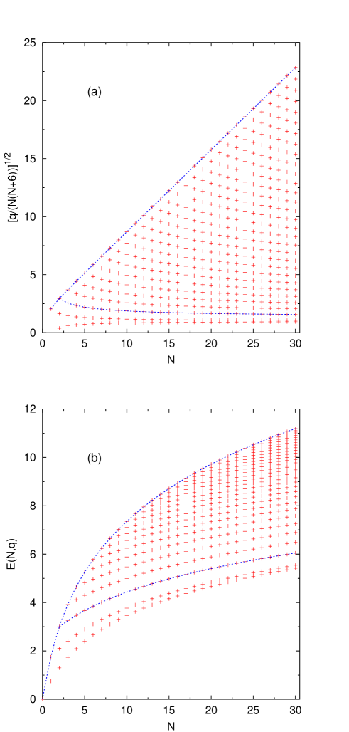
Figure 1: The dependence of the quantized values of the charge $q$ and the energy ${\cal E}(N,q)$ on the spin $N$ for the values of the impurity parameters $\omega_{1}=\omega_{3}=3/2$ corresponding to the evolution kernel ${\cal H}_{T}$. The dotted lines represent two trajectories with $\bar{\ell}=0$ (upper curve) and $\ell=3$ (lower curve) described in Sect. 7.4.

The results of the numerical solution of the recurrence relations for the charge $q$ and the energy ${\cal E}(N,q)$ and their dependence on the spin $N$ and the impurity parameters $\omega_{1,3}$ are shown in Figs. 1 and 2, respectively. We observe from Figs. 1 that the eigenvalues of the charge $q$ and the energy ${\cal E}(N,q)$ grow with the spin $N$ and occupy the band [14]

$$q_{\rm min}(N)<q<q_{\rm max}(N)\,,\qquad{\cal E}_{\rm min}(N)<{\cal E}(N,q)<{\cal E}_{\rm max}(N)$$ (6.41)

with $q_{\rm min}={\cal O}(N^{2})$, ${\cal E}_{\rm min}\sim 2\ln N$ and $q_{\rm max}={\cal O}(N^{4})$, ${\cal E}_{\rm max}\sim 4\ln N$. In addition, the spectrum of $q$ and ${\cal E}(N,q)$ exhibit an interesting properties of regularity. To understand these properties we shall apply in the next section the asymptotic methods to find an approximate solution to the Baxter equation for large values of the spin $N$.

6.2.3. Singular states

According to (6.38) the solutions to the recurrence relations depend on the shift parameters $\omega_{k}$. Examining the dependence of the energy (6.39) on $\omega_{1}$ and $\omega_{3}$ shown in Fig. 2a one observes that ${\cal E}(N,q)$ diverges as $\omega_{k}$ approaches half-integer values

$$\omega_{\rm sing}=\pm\frac{5}{2}\,,\pm\frac{7}{2}\,,...\,,\pm\left(\frac{3}{2}+N\right)\,.$$ (6.42)

The total number of the singular points is equal to the spin $N$. As $N$ increases they start to occupy the whole real axis except of the interval

$$-\frac{5}{2}<\omega_{1,3}<\frac{5}{2}\,,$$ (6.43)

which defines the stability region of the model.

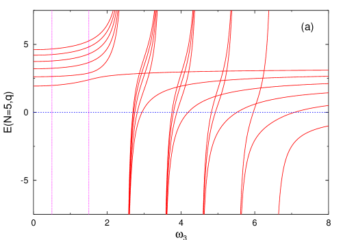
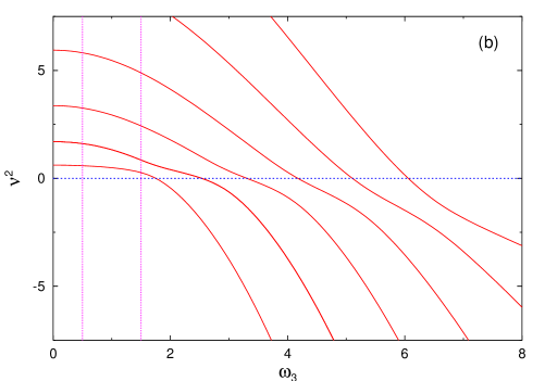
Figure 2: The flow of the energy ${\cal E}(N,q)$ and the conserved charge $q=2N(N+6)(\nu^{2}+3/4)$ with $\omega_{3}$ for $N=5$ and $\omega_{1}=3/2$. Two vertical dotted lines correspond to $\omega_{3}=1/2$ and $\omega_{3}=3/2$ and define the spectrum of the evolution kernels ${\cal H}_{S}$ and ${\cal H}_{T}$, respectively.

This phenomenon can be understood by noticing that the two-particle energy in the $(12)-$channel entering (6.39) diverges as $\omega_{k}\to\omega_{\rm sing}$ due to singularities of the $\psi-$functions. Taking $\omega_{1}=5/2+n$ with $n=0\,,1\,,...$ we find from (6.39) that divergence comes from the contribution of two particle spins $k=n+1$, $...$, $N$. As a consequence, for this value of $\omega_{1}$ the only levels in the spectrum that have a finite energy are those with $u_{k}=0$ for $k=n+1$, $...$, $N$. If this condition is not satisfied the energy becomes infinite. For $\omega_{1}=5/2+n$ the total number of finite energy states is equal to $n+1$ and at $n=N$ there are no divergent states left in the spectrum. Since the finite energy states form an orthogonal subspace, the singular states have $u_{k}/u_{N}=0$ for $k=0$, $...$, $n$.

According to (6.9), the existence of the singular states corresponds to appearance of the Bethe roots at $\lambda_{k}=\pm 3i/2$.

7. Asymptotic solution of the Baxter equation

Although the Baxter equation (6.7) can not be solved exactly there is a simple way to find its asymptotic solutions at large values of the spin $N$ [29]. The method is based on the observation that the both sides of the Baxter equation (4.19) have a different scaling behaviour at large $N$. We find that for $u={\rm fixed}$ the l.h.s. of (4.19) scales as $\Delta_{\pm}(u)\sim N^{0}$ whereas its r.h.s. involves the transfer matrix (6.6) that grows at large $N$ as

$$\widehat{t}_{-1/2}(u)={\cal O}(q)$$ (7.1)

depending to the value of the charge $q(N)$, Eq. (6.41). Then, introducing the function

$${\bf\varphi}(u)=\frac{{\mathbf{Q}}(u+i)}{{\mathbf{Q}}(u)}$$ (7.2)

one rewrites the Baxter equation (4.19)

$$\frac{\Delta_{+}(u)}{\varphi(u-i)}+\Delta_{+}(-u)\,\varphi(u)=\widehat{t}_{-1/2}(u)\,.$$ (7.3)

A general solution to this relation is given by (an infinite) continuous fraction. Taking into account (7.1) we find that at large $N$ and $u={\rm fixed}$ the solutions to (7.3) are given by

$$\varphi_{+}(u) = \frac{\Delta_{+}(u+i)}{\widehat{t}_{-1/2}(u+i)}+{\cal O}(1/q^{2})\,,$$ (7.4)

$$\varphi_{-}(u) = \frac{\widehat{t}_{-1/2}(u)}{\Delta_{+}(-u)}+{\cal O}(1/q)\,.$$ (7.5)

It is easy to verify that these relations lead to the following expressions for the ${\mathbf{Q}}-$function

$${\mathbf{Q}}_{+}(u) = 2^{iu}\frac{\Gamma(iu)}{\Gamma(iu-\frac{1}{2})}\prod_{k=1}^{3}\frac{\Gamma(i(u+\sigma_{k}))\Gamma(i(u-\sigma_{k}))}{\Gamma(iu+j_{k}^{+})\Gamma(iu+j_{k}^{-})}$$ (7.6)

$${\mathbf{Q}}_{-}(u) = {\mathbf{Q}}_{+}(-u)\,,$$ (7.7)

where $j_{k}^{\pm}$ were defined in (3.15) and $\sigma_{k}$ denote the roots of the transfer matrix (6.6)

$$\widehat{t}_{-1/2}(u)=-2\prod_{k=1}^{3}(u^{2}-\sigma_{k}^{2})\,.$$ (7.8)

The general solution to the Baxter equation is given by a linear combination of ${\mathbf{Q}}_{\pm}(u)$. Requiring ${\mathbf{Q}}(u)$ to be an even function of $u$ one gets

$${\mathbf{Q}}_{\rm as}(u)={\mathbf{Q}}_{+}(u)+{\mathbf{Q}}_{-}(u)={\mathbf{Q}}_{+}(u)+{\mathbf{Q}}_{+}(-u)\,.$$ (7.9)

We would like to stress that thus defined asymptotic ${\mathbf{Q}}-$function obeys the Baxter equation (6.7) only in the limit $N\to\infty$ and $u={\rm fixed}$ up to ${\cal O}(1/q)-$corrections.

The dependence of the ${\mathbf{Q}}-$function on the charge $q$ enters into (7.9) through the roots $\sigma_{k}$ of the transfer matrix, Eq. (7.8). Since large scales, $q$ and $N(N+6)$, appear in (6.6) with a common prefactor $(u^{2}+1/4)$, one of the roots is $q-$independent and it is given by

$$\sigma_{2}^{2}=-\frac{1}{4}+{\cal O}(N^{-2})\,.$$ (7.10)

Then, taking into account the values of the parameters $j_{k}^{\pm}$ one simplifies (7.6) as

$${\mathbf{Q}}_{+}(u)=2^{iu}\frac{\Gamma(iu)\Gamma(iu+\frac{1}{2})}{\Gamma^{2}(iu+\frac{3}{2})}\prod_{k=1,3}\frac{\Gamma(iu-i\sigma_{k})\Gamma(iu+i\sigma_{k})}{\Gamma(iu+1-\omega_{k})\Gamma(iu+1+\omega_{k})}\,.$$ (7.11)

The values of the remaining roots $\sigma_{1,3}$ vary significantly as the charge $q$ changes inside the band (6.41).

Close to the upper bound $q={\cal O}(N^{4})$ one finds that the both roots are real and increase with the spin $N$ as

$$\sigma_{1,3}^{2}=\left[1\pm\sqrt{1-\bar{q}}\right]N(N+6)+{\cal O}(N^{0})\,,$$ (7.12)

where $\bar{q}=q/(N(N+6))^{2}={\cal O}(N^{0})$.

Close to the lower bound $q={\cal O}(N^{2})$ one finds that one of the roots is $N-$independent

$$\sigma_{1}^{2}=2N(N+6)+{\cal O}(N^{0})\,,\qquad\sigma_{3}^{2}=\nu^{2}+{\cal O}(N^{-2})\,,$$ (7.13)

where the parameter $\nu$ is defined as

$$\nu^{2}=\frac{q}{2N(N+6)}-\frac{3}{4}={\cal O}(N^{0})\,.$$ (7.14)

Notice that $\nu$ takes real values for $q\geq 3N(N+6)/2$ and it becomes pure imaginary for $q<3N(N+6)/2$. This happens in particular for the exact levels, Eqs.(6.12) and (6.19)

$$(\nu^{(\pm)}_{T})^{2}=-\frac{1}{4}\mp\frac{2}{N}+{\cal O}(N^{-2})\,,\qquad\nu^{2}_{S}=-\frac{1}{4}+{\cal O}(N^{-2})\,.$$ (7.15)

As we will see later, the appearance of the complex roots of the transfer matrix is closely related to the existence of the mass gap in the spectrum of the Hamiltonian.

7.1. Dispersion curve

Let us apply the solution (7.9) to obtain the asymptotic expression for the energy ${\cal E}$. According to (6.9) the energy is determined by a logarithmic derivative of the ${\mathbf{Q}}-$function at $u=\pm 3i/2$. These values of $u$ belong to the applicability region of the asymptotic solutions, $N\to\infty$ and $u={\rm fixed}$, and therefore one is allowed to replace ${\mathbf{Q}}-$function in (6.9) by its asymptotic expression (7.9).

It follows from (7.11) that ${\mathbf{Q}}_{\pm}(\pm 3i/2)=0$ and close to $u=\pm 3i/2$ the ${\mathbf{Q}}-$function is given by one of the functions, ${\mathbf{Q}}={\mathbf{Q}}_{\pm}(u)$. Substitution of (7.9) into (6.9) yields

$${\cal E}_{\rm as}(N,q)=\sum_{k=1,3}\left[\psi\left(\mbox{$\frac{3}{2}$}+i\sigma_{k}\right)+\psi\left(\mbox{$\frac{3}{2}$}-i\sigma_{k}\right)\right]-\ln 2-\varepsilon(\omega_{1},\omega_{3})+{\cal O}(1/q)\,,$$ (7.16)

where the notation was introduced for the normalization constant

$$\varepsilon(\omega_{1},\omega_{3})=\sum_{k=1,3}\psi\left(\mbox{$\frac{5}{2}$}+\omega_{k}\right)+\psi\left(\mbox{$\frac{5}{2}$}-\omega_{k}\right)$$ (7.17)

and $\sigma_{1,3}$ are nontrivial roots of the transfer matrix defined in Eqs. (7.8) and (6.6). The explicit expressions for $\sigma_{1,3}$ are quite cumbersome and one can use instead the approximate expression

$$\sigma_{1,3}^{2}=\left[1\pm\sqrt{1-\widetilde{q}}\right]N(N+6)+{\cal O}(N^{0})\,,\qquad\widetilde{q}=\frac{q-\frac{3}{2}N(N+6)}{[N(N+6)]^{2}}\,,$$ (7.18)

which agrees with the asymptotic expressions (7.12) and (7.13). The relation (7.16) establishes the dependence of the energy on the integrals of motion, $N$ and $q$, and provides an explicit expression for the dispersion curve of the spin chain model.

The expression (7.16) simplifies in the upper part of the spectrum (6.41). We find using (7.12) and (7.13) that

$${\cal E}_{\rm as}(N,q)=\ln(q/2)-\varepsilon(\omega_{1},\omega_{3})+{\cal O}(N^{-2})$$ (7.19)

provided that $q={\cal O}(N^{4})$.

In the lower part of the spectrum we get from (7.13)

$${\cal E}_{\rm as}(N,q)=\ln[N(N+6)]+\psi\left(\frac{3}{2}+i\nu\right)+\psi\left(\frac{3}{2}-i\nu\right)-\varepsilon(\omega_{1},\omega_{3})+{\cal O}(N^{-2})$$ (7.20)

with $\nu^{2}=q/(2N(N+6))-3/4={\cal O}(N^{0})$. For the special values of the impurity parameters, Eqs. (3.21) and (3.22), the relations (7.19) and (7.20) coincide with analogous expressions obtained in [4, 14].

Since $\nu$ could be either real or pure imaginary in (7.20), we separate the corresponding energy levels into two groups by introducing the “vacuum” energy

$${\cal E}_{\rm vac}(N)=\ln[N(N+6)]+2\psi\left(\mbox{$\frac{3}{2}$}\right)-\varepsilon(\omega_{1},\omega_{3})\,.$$ (7.21)

The energy levels with $\nu^{2}\geq 0$ lie above the vacuum, ${\cal E}_{\rm as}(N,q)\geq{\cal E}_{\rm vac}(N)$, and we shall refer to them as “continuum”, while a few lowest energy levels with $\nu^{2}<0$ and ${\cal E}_{\rm as}(N,q)<{\cal E}_{\rm vac}(N)$ correspond to the “bound states”.

As we will show in Sect. 7.2.1 (see Eq. (7.30) below), the parameters $\nu$ scale in the continuum at large $N$ as $\nu\sim 1/\ln N$. For small real $\nu$ one expands the r.h.s. of (7.20) in powers of $\nu$ and finds that the energy in the continuum grows linearly with $q$ close to ${\cal E}_{\rm vac}$

$${\cal E}_{\rm continuum}(N,q)-{\cal E}_{\rm vac}(N)=\left[\frac{q}{N(N+6)}-\frac{3}{2}\right](8-7\zeta(3))\,.$$ (7.22)

The energy of the bound states has a completely different behaviour at large $N$ because in contrast with the continuum the parameter $|\nu|$ takes finite values for these states. As a consequence, their energy levels are separated from the continuum by a gap

$$\Delta{\cal E}={\cal E}_{\rm vac}(N)-{\cal E}_{\rm bound}(N,q)=2\psi\left(\frac{3}{2}\right)-\psi\left(\frac{3}{2}+|\nu|\right)-\psi\left(\frac{3}{2}-|\nu|\right)\,.$$ (7.23)

We will estimate the value of the mass gap at large $N$ in Sect. 7.2.3.

The asymptotic expansions (7.16), (7.19) and (7.20) are valid up to corrections vanishing at large $N$. Let us check the accuracy of (7.16) by comparing ${\cal E}_{\rm as}(N,q)$ with the exact values of the energy obtained from the solution of the recurrence relations, Eqs. (6.39) and (6.38). To this end we choose the shift parameters to correspond to the QCD evolution kernel (3.22), $\omega_{1}=\omega_{3}=3/2$, and take the spin to be $N=10$. Applying (6.38) and (6.39) we find $N+1$ pairs of the exact eigenvalues $(q,{\cal E}_{\rm ex})$ that we compare with the dispersion curve ${\cal E}_{\rm as}(N,q)$ as shown in Fig. 3. Calculating the difference $\delta{\cal E}={\cal E}_{\rm as}(N,q)-{\cal E}_{\rm ex}(N,q)$ we find that the asymptotic formula (7.16) reproduces the exact energy with a very high accuracy $\delta{\cal E}<10^{-5}$, which increases up to $\delta{\cal E}<10^{-8}$ as one goes from the lower part of the spectrum to the upper bound by increasing $q$.

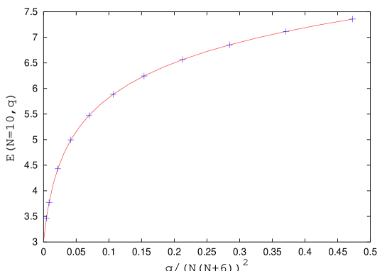
Figure 3: The dependence on the energy ${\cal E}(N,q)$ on the conserved charge $q$ at $N=10$. Crosses denote the exact values of the energy and the solid line corresponds to the asymptotic expression (7.16).

7.2. Quantization of the conserved charge

Let us show that the matching of the analytical properties of the asymptotic solutions (7.9) into Eq. (6.8) leads to the quantization conditions on the charge $q$.

It follows from (7.9) and (7.11) that the function ${\mathbf{Q}}_{\rm as}(u)$ has an infinite series of poles in the complex $u-$plane generated by $\Gamma-$functions in the numerator of (7.11) and located at

$$u_{\rm pole}=\left\{\pm\frac{i}{2}\,,\ n\,,\ \pm\sigma_{1}+in\,,\ \pm\sigma_{3}+in\right\}$$ (7.24)

with $n$ being arbitrary integer. This seems to be in contradiction with the fact that the exact solutions to the Baxter equation are given by polynomials in $u$, Eq. (6.8). Notice however that the asymptotic and the exact solutions for ${\mathbf{Q}}(u)$ should coincide (up to corrections vanishing at large $N$) only in a finite region of $u$ whereas some poles in (7.24) are moved outside this region as $N\to\infty$. This allows to remove from the consideration the “moving” poles in (7.24) satisfying the condition $u_{\rm pole}={\cal O}(N)$ and keep only the “fixed” poles, $u_{\rm pole}={\cal O}(N^{0})$. In particular, in the upper part of the spectrum we get from (7.12) that $\sigma_{1,3}={\cal O}(N)$ and therefore the fixed poles of ${\mathbf{Q}}(u)$ are located at

$$u_{\rm fixed~{}pole}\bigg{|}_{q={\cal O}(N^{4})}=\left\{\pm\frac{i}{2}\,,\ in\right\}\,.$$ (7.25)

Similarly in the lower part of the spectrum we use (7.13) and (7.24) to find the fixed poles of (7.11) as

$$u_{\rm fixed~{}pole}\bigg{|}_{q={\cal O}(N^{2})}=\left\{\pm\frac{i}{2}\,,\ in\,,\ \pm\nu+in\right\}$$ (7.26)

with $\nu$ defined in (7.14) and $n=\rm integer$.

Let us now examine the residue of ${\mathbf{Q}}_{\rm as}(u)$ at the fixed poles (7.25) in the upper part of the spectrum. Using the explicit expression for the functions ${\mathbf{Q}}_{+}(u)$, Eq. (7.11), one finds that at large $N$ the residue of ${\mathbf{Q}}_{+}(u)$ at $u=im$ with $m=\frac{1}{2}\,,1\,,2\,,...$ is suppressed with respect to its residue at $u=0$ by a factor $(\sigma_{1}\sigma_{3})^{-4m}={\cal O}(q^{-2m})$ that vanishes as $N\to\infty$. Therefore up to ${\cal O}(1/q)-$corrections one can neglect in (7.25) the fixed poles at $u=\pm\frac{i}{2}$ and $u=in$ and keep only the leading pole at $u=0$.

Repeating similar consideration for the fixed poles in the lower part of the spectrum, (7.26), one finds that only the poles at $u=0$ and $u=\pm\nu$ survive in the large $N$ limit provided that $|{\rm Im}\,\nu|<1/2$. Notice that the residue of ${\mathbf{Q}}(u)$ at $u=\pm\nu$ scales as $\sim q^{\mp 2i\nu}$ and for $|{\rm Im}\,\nu|\geq 1/2$ it becomes comparable with the contribution of subleading poles at $u=\pm i/2$ and $u=in\neq 0$. Thus, in order to match the asymptotic solution (7.9) into (6.8) one has to require that ${\mathbf{Q}}(u)$ should have a zero residue at $u=0$. In addition, in the lower part of the spectrum one has to impose the same condition at $u=\pm i\nu$.

It is easy to see from (7.6) that the residue of ${\mathbf{Q}}_{+}(u)$ and ${\mathbf{Q}}_{-}(u)$ at $u=0$ cancel each other in the sum (7.9) independently on the value of the charge $q$. At the same time, calculating the residue of (7.9) and (7.11) at $u=\pm i\nu$ we find after some algebra that it vanishes provided that $\nu$ obeys the following equation

$$\left[N(N+6)\right]^{-2i\nu}=\frac{\Gamma^{2}(1+2i\nu)\Gamma^{2}(\frac{3}{2}-i\nu)}{\Gamma^{2}(1-2i\nu)\Gamma^{2}(\frac{3}{2}+i\nu)}\prod_{k=1,3}\frac{\Gamma(1+\omega_{k}-i\nu)\Gamma(1-\omega_{k}-i\nu)}{\Gamma(1+\omega_{k}+i\nu)\Gamma(1-\omega_{k}+i\nu)}\,,$$ (7.27)

where $\nu^{2}=q/(2N(N+6))-3/4$. This relation establishes the quantization condition on the charge $q$ in the lower part of the spectrum $q={\cal O}(N^{2})$.

Solving the quantization conditions (7.27) we distinguish two cases: the states in the continuum, $\nu^{2}>0$, and the bound states, $\nu^{2}<0$.

7.2.1. Solving the quantization conditions in continuum

For $\nu^{2}>0$ one gets from (7.27)

$$\nu\ln N(N+6)-{\rm arg}\,\frac{\prod_{k=1,3}{\Gamma(1+\omega_{k}+i\nu)\Gamma(1-\omega_{k}+i\nu)}}{\Gamma^{2}(1+2i\nu)\Gamma^{2}(\frac{3}{2}-i\nu)}=\pi\ell$$ (7.28)

with $\ell$ being an integer. For the special values of the impurity parameters, Eqs. (3.21) and (3.22), this relation coincides with the quantization conditions obtained in [4, 14].

It follows from (7.28) that $\nu$ scales as $\nu\sim c/\ln[N(N+6)]$ at large $N$ with the constant $c$ having a nontrivial dependence on the impurity parameters $\omega_{1}$ and $\omega_{3}$. In particular, varying these parameters one finds that $c$ gets a finite contribution as $\omega_{1,3}$ passes through integer values. To show this we use the identity

$${\rm arg}\,\Gamma(1-\omega_{k}+i\nu)={\rm arg}\,\Gamma(2-\omega_{k}+i\nu)-{\rm arg}\,(1-\omega_{k}+i\nu)$$ (7.29)

and notice that as $\omega_{k}$ passes through the value $\omega_{k}=1$ the phase of $(1-\omega_{k}-i\nu)$ changes by $\pi$. This transition occurs in the region $|1-\omega_{k}|={\cal O}(\nu)={\cal O}(1/\ln[N(N+6)])$. In a similar manner, changing $\omega_{k}$ from $1$ to $\infty$ we find that every time $\omega_{k}$ passes integer positive values the l.h.s. of (7.28) increases by $\pi$, or equivalently the integer $\ell$ in the r.h.s. of (7.28) decreases as $\ell\to\ell-1$. As we will see in a moment, this effect corresponds to formation of the bound state which “dives” below the vacuum energy and causes reparameterization of the levels in the continuum.

For $0\leq\omega_{1}\,,\omega_{3}<1$ and $1-\omega_{1,3}\gg 1/\ln[N(N+6]$ we obtain the solution to (7.28) as

$$\nu_{0}(\ell)=\frac{\pi\ell}{\ln[N(N+6)]+C}+{\cal O}\left(\frac{\ell^{3}}{\ln^{3}N}\right)$$ (7.30)

with

$$C=4\psi(1)-2\psi(\mbox{$3\over 2$})-\sum_{k=1,3}\left[\psi(1-\omega_{k})+\psi(1+\omega_{k})\right]\,.$$

Substituting (7.30) into (7.20) we find the energy of the $\ell-$th level as

$${\cal E}_{\ell}={\cal E}_{\rm vac}+(14\,\zeta(3)-16)\frac{\pi^{2}\ell^{2}}{\ln^{2}[N(N+6)\,\mbox{e}^{C}]}+{\cal O}\left(\frac{\ell^{4}}{\ln^{4}N}\right)$$ (7.31)

with the vacuum energy ${\cal E}_{\rm vac}$ given by (7.21). Integer $\ell=1\,,2\,,...$ enumerates the energy levels with $\ell=1$ being the lowest level in the continuum. Note that this expression is valid only for the lowest $l\sim\ln[N(N+6)]$ states. Using (7.31) we find the level spacing in the continuum close to the vacuum level as

$$\delta{\cal E}_{l}(N)\stackrel{{\scriptstyle\nu\to 0}}{{=}}{\cal O}\left(\frac{1}{\ln^{2}[N(N+6)]}\right)\,.$$ (7.32)

Let us now increase $\omega_{1}$ and keep $\omega_{3}$ unchanged. We find from (7.31) that the energy of all levels increases (see Fig. 2a) while the difference ${\cal E}_{\ell}-{\cal E}_{\rm vac}$ decreases with $\omega_{1}$ (see Fig.4a). The lowest level ${\cal E}_{\ell=1}$ rapidly approaches the vacuum energy ${\cal E}_{\rm vac}$ as $\omega_{1}\to 1$. Once $\omega_{1}$ crosses the value $\omega_{1}=1$ one applies (7.29) to obtain the solution to (7.28) as

$$\nu(\ell)\bigg{|}_{1<\omega_{1}<2\atop 0<\omega_{3}<1}=\nu_{0}(\ell-1)$$ (7.33)

with $\ell\geq 1$ and $\nu_{0}(\ell)$ given by (7.30). Thus, the lowest energy level $\ell=1$ disappears from the continuum and this induces reparameterization of the remaining levels, $\ell\to\ell-1$. Since this effect occurs every time as $\omega_{1}$ or $\omega_{3}$ passes through integer values it is now easy to write the general solution to (7.28) valid for arbitrary values of $\omega_{1,3}$

$$\nu(\ell)\bigg{|}_{\omega_{1},\,\omega_{3}>0}=\nu_{0}(\ell-[\omega_{1}]-[\omega_{3}])\,,$$ (7.34)

where $[\omega_{k}]$ denotes an integer part of $\omega_{k}$. We conclude that as a result of the flow of the spectrum of the model from $\omega_{1}=\omega_{3}=0$ to arbitrary $\omega_{1,3}$,

$${\cal N}_{\rm bound}=[\omega_{1}]+[\omega_{3}]$$ (7.35)

states cross the vacuum level with $\nu_{\rm vac}=0$ and the energy ${\cal E}_{\rm vac}$ and disappear from the continuum. These levels have the charge $\nu^{2}<0$, or equivalently $q<3N(N+6)/2$, and they can be described using (7.27).

7.2.2. Solving the quantization conditions for the bound states

For $\nu^{2}<0$ we put $\nu=i\rho$ with $\rho>0$ and examine the large $N$ behavior of the both sides of (7.27). The l.h.s. of (7.27) grows as $\sim N^{4\rho}$ whereas the r.h.s. is a meromorphic $N-$independent function of $\rho$. Therefore in the limit $N\to\infty$ one could satisfy (7.27) either through a trivial solution $\rho\sim 1/\ln[N(N+6)]$, or taking $\rho$ to be close to the poles of the r.h.s.

We find using (7.27) that for $\rho>0$ and $0<\omega_{1,3}<1$ the poles are located at $\rho=1/2$ and $\rho={\rm positive\ integer}$. However, these poles coincide with the subleading fixed poles in (7.26) and their contribution is beyond an approximation at which (7.27) was obtained.

Increasing the values of the impurity parameter $\omega_{1}>1$ we observe that the r.h.s. of (7.27) develops the poles at

$$\rho=\omega_{1}-1\,,\omega_{1}-2\,,...\,,\{\omega_{1}-1\}$$ (7.36)

with $\{\omega_{1}-1\}$ being a fractional part of $\omega_{1}$. Similar phenomenon occurs as one increases the parameter $\omega_{3}$. Then, for arbitrary positive $\omega_{1}$ and $\omega_{3}$ the total number of the poles is equal to $[\omega_{1}]+[\omega_{3}]$ and coincides with the number of the “missing” levels from the continuum ${\cal N}_{\rm bound}$. Thus, at large $N$ Eq. (7.27) has two branches of the solutions each parameterized by integers $n_{1}$ and $n_{3}$, respectively

$$i\nu=n_{k}+\{\omega_{k}-1\}+{\cal O}\left(N^{-1}\right)$$ (7.37)

with $k=1,3$ and $n_{k}=1\,,...\,,[\omega_{k}-1]$. To find ${\cal O}(1/N)$ corrections to these expressions one has to include subleading corrections to the quantization condition (7.27), or equivalently to the asymptotic solution (7.9) and (7.6). Each solution (7.37) corresponds to the bound state with the energy ${\cal E}_{\rm bound}(n_{1})$ or ${\cal E}_{\rm bound}(n_{3})$ given by

$${\cal E}_{\rm vac}-{\cal E}_{\rm bound}(n_{k})=2\psi\left(3\over 2\right)-\psi\left({3\over 2}+n_{k}+\{\omega_{k}-1\}\right)-\psi\left({3\over 2}-n_{k}-\{\omega_{k}-1\}\right)+{\cal O}\left(N^{-1}\right)$$ (7.38)

with $0\leq n_{k}\leq[\omega_{k}-1]$. Thus, as $\omega_{k}$ passes through an integer $n_{k}$ the level from continuum (7.31) with the energy ${\cal E}_{\ell=n_{k}}$ crosses the vacuum to transform into the bound state with the energy ${\cal E}_{\rm bound}(n_{k})$. This transition occurs in the region $|\omega_{k}-n_{k}|={\cal O}(1/\ln N)$ and it is clearly seen on Fig. 4a. For given $\omega_{1}$ and $\omega_{3}$ the total number of bound states is equal to (7.35). Note that up to ${\cal O}(1/N)$ corrections the difference ${\cal E}_{\rm vac}-{\cal E}_{\rm bound}$ does not depend on the spin $N$.

In particular, using (7.35) and (7.37) we find that for $\omega_{1}=1/2\,,$ $\omega_{3}=3/2$ and $\omega_{1}=\omega_{3}=3/2$ the spectrum contains ${\cal N}_{\rm bound}=1$ and ${\cal N}_{\rm bound}=2$ bound states, respectively, with $i\nu=-1/2+{\cal O}(1/N)$. In the second case, two bound states are degenerate up to ${\cal O}(1/N)$ corrections. This is in agreement with the exact results (6.23) and (6.15).

7.2.3. Mass gap

We observe from Figs. 1b and 4b that at large $N$ and fixed $\omega_{1,3}$ the bound states are separated from the continuum by a finite mass gap, $\Delta(\omega_{1},\omega_{3})={\rm min}\left({\cal E}_{\ell}-{\cal E}_{\rm bound}\right)$. We estimate its value using (7.31) and (7.38) as

$$\Delta(\omega_{1},\omega_{3})={\cal E}_{\rm vac}-{\rm max}_{n_{1},n_{2}}\,{\cal E}_{\rm bound}(n_{k})+{\cal O}(1/\ln^{2}N)\,.$$ (7.39)

Then, $\Delta(\omega_{1},\omega_{3})=0$ for $0<\omega_{1,3}<1$ and

$$\Delta(\omega_{1},\omega_{3})=2\psi\left(3\over 2\right)-\psi\left({3\over 2}+\{\omega_{1}-1\}\right)-\psi\left({3\over 2}-\{\omega_{1}-1\}\right)$$ (7.40)

both for $0<\omega_{3}<1<\omega_{1}$ and for $1<\omega_{1}\leq\omega_{3}$.

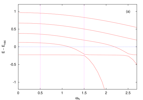
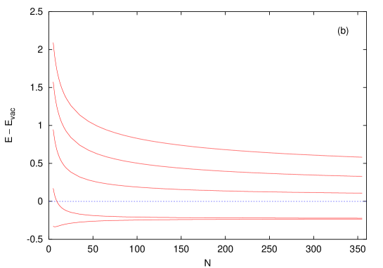
Figure 4: The difference ${\cal E}(N,q)-{\cal E}_{\rm vac}(N)$ for the lowest five energy levels of the Hamiltonian ${\cal H}(\omega_{1},\omega_{3})$: (a) the dependence on the impurity $\omega_{3}$ for $N=100$ and $\omega_{1}=3/2$; (b) the dependence on the spin $N$ for $\omega_{1}=\omega_{3}=3/2$.

Applying (7.40) for the values of parameters $\omega_{1,3}$ corresponding to the QCD evolution kernel, (3.22) and (3.21), one calculates the mass gap as

$$\Delta\left(\frac{3}{2},\frac{1}{2}\right)=\Delta\left(\frac{3}{2},\frac{3}{2}\right)=2\psi\left(\mbox{$\frac{3}{2}$}\right)-\psi(1)-\psi(2)=3-4\ln 2=0.227411\,.$$ (7.41)

This result agrees with the exact calculations of the difference ${\cal E}(N,q)-{\cal E}_{\rm vac}(N)$ at $\omega_{1}=\omega_{3}=3/2$ as shown in Fig. 4. Note that (7.41) is valid up to corrections $\sim\pi^{2}/\ln^{2}[N(N+6)\mbox{e}^{C}]$ which decrease slowly with $N$ and provide a sizeable contribution to $\Delta$ at finite $N$.

According to (7.41) the mass gaps in the spectrum of the QCD evolution kernels, ${\cal H}_{T}$ and ${\cal H}_{S^{+}}$, are the same. Nevertheless, the energies of bound state for these two Hamiltonians are different due to dependence of the vacuum energy on the shift parameters, Eqs. (7.21) and (7.17). Their difference is given by

$${\cal E}_{T,{\rm bound}}-{\cal E}_{S,{\rm bound}}={\cal E}_{\rm vac}\left(\frac{3}{2},\frac{1}{2}\right)-{\cal E}_{\rm vac}\left(\frac{3}{2},\frac{3}{2}\right)=\frac{2}{3}$$ (7.42)

and it coincides with the exact result (6.24).

To summarize, matching the asymptotic solution (7.9) into the exact form (6.8) at large $N$ and $u={\rm fixed}$ we obtained the quantization conditions (7.27) and used them to calculate the asymptotic expansion of the charge $q$ and the energy ${\cal E}(N,q)$ in the lower part of the spectrum, Eqs. (7.31) and (7.38), and estimated the value of the mass gap, Eqs. (7.40) and (7.41). To find similar expansion in the upper part of the spectrum one needs an asymptotic solution to the Baxter equation that is valid at large $N$ and $u={\cal O}(N)$.

7.3. WKB expansion

Analyzing the Baxter equation (4.19) at large $N$ and $u={\cal O}(N)$ it is convenient to introduce the scaling variables

$$u=\eta x\,,\qquad\eta^{2}=N(N+6)\,,\qquad\bar{q}=q/(N(N+6))^{2}\,.$$ (7.43)

Then, one gets from (6.5) and (6.6)

$$\Delta_{+}(\eta x)=-\eta^{6}x^{6}\left[1+i\frac{s}{x}{\eta^{-1}}+{\cal O}(\eta^{-2})\right]$$ (7.44)

with $s=1/2-2\sum_{k}j_{k}=-13/2$ and

$$\widehat{t}_{-1/2}(\eta x)=2\eta^{6}x^{6}\left[V_{0}(x)-1+{\cal O}(\eta^{-2})\right]\,,\qquad V_{0}=2/x^{2}-\bar{q}/x^{4}\,.$$ (7.45)

Substituting these relations into (4.19) one observes that in the leading $\eta\to\infty$ limit the Baxter equation takes the form of the discretized one-dimensional Schrödinger equation on the “wave function” ${\mathbf{Q}}(x\eta)$. In this equation the parameter $1/\eta$ plays the rôle of the Planck constant and $V_{0}(x)$ defines the potential. This suggests to look for its solutions in the WKB form [33]

$${\mathbf{Q}}_{+}(x\eta)=\exp\left(i\eta S(x)\right)\,,\qquad S(x)=S_{0}(x)+\eta^{-1}S_{1}(x)+{\cal O}(\eta^{-2})\,,$$ (7.46)

where $S_{0}(x)$, $S_{1}(x)$, $...$ are $\eta-$independent and the expansion is assumed to be uniformly convergent. Substituting the WKB ansatz (7.46) into the Baxter equation (4.19) one expands its both sides in powers of $1/\eta$ to get

$$\cosh S_{0}^{\prime}(x)=1-V_{0}(x)\,,\qquad S_{1}^{\prime}(x)=\frac{i}{2}S_{0}^{\prime\prime}(x)\coth S_{0}^{\prime}(x)-i\frac{s}{x}\,,\ ...$$ (7.47)

This leads to the following WKB expansion

$${\mathbf{Q}}_{+}(x\eta)=\frac{x^{s}}{\sqrt{\sinh S_{0}^{\prime}(x)}}\exp\left(i\eta\int^{x}d\xi\,S_{0}^{\prime}(\xi)+{\cal O}(\eta^{-1})\right)$$ (7.48)

with $S_{0}^{\prime}(x)$ satisfying (7.47). Finally, combining together (7.9) and (7.48) we arrive at the asymptotic expansion of the Baxter equation solution that is valid at large $N$ and $u=x\eta={\cal O}(N)$.

Performing the matching of (7.9) and (7.48) into the exact solution (6.8), we shall impose the following two conditions: the asymptotic solution ${\mathbf{Q}}_{\rm WKB}(x\eta)$ should be a single valued function of $x$ and it should oscillate on the real $x-$axis in order for ${\mathbf{Q}}-$function to have the real Bethe roots $\lambda_{k}={\cal O}(N)$.

Exploring the interpretation of ${\mathbf{Q}}_{\rm WKB}(x\eta)$ as a quantum-mechanical WKB wave function we obtain in the standard way that the first requirement is translated into the Borh-Sommerfeld quantization condition on the eikonal phase

$$\frac{1}{2\pi i}\oint dS(x)=\frac{1}{\pi}\int_{x_{-}}^{x_{+}}dx\,S^{\prime}(x)=\bar{\ell}\eta^{-1}\,,$$ (7.49)

where $\bar{l}$ is a nonnegative integer and the integration is performed over a closed contour on the complex $x-$plane encircling the classical interval of motion $x_{-}\leq x\leq x_{+}$ defined as

$$\left(1-V_{0}(x_{\pm})\right)^{2}=\left(1-2x^{-2}_{\pm}+\bar{q}x^{-4}_{\pm}\right)^{2}=1\,.$$ (7.50)

Replacing $S=S_{0}+S_{1}/\eta$ and using (7.47) we get from (7.49)

$$\frac{1}{\pi}\int_{x_{-}}^{x_{+}}dx\,S_{0}^{\prime}(x)=\left(\bar{\ell}+\frac{1}{2}\right)\eta^{-1}+{\cal O}(\eta^{-2})\,.$$ (7.51)

Since the WKB wave function oscillates on the interval $[x_{-},x_{+}]$ we can satisfy the second requirement by demanding $x_{-}$ and $x_{+}$ to be real. This leads to the following constraint on the possible values of the charge $\bar{q}=q/[N(N+6)]^{2}$

$$0<\bar{q}\leq\frac{1}{2}\,.$$ (7.52)

Moreover, solving the Borh-Sommerfeld quantization conditions (7.51) one can develop the asymptotic expansion of the charge $q$ close to the upper bound, $\bar{q}={\cal O}(N^{0})$

$$\bar{q}=q/[N(N+6)]^{2}=q^{(0)}+\frac{q^{(1)}}{\eta}+\frac{q^{(2)}}{\eta^{2}}+\frac{q^{(3)}}{\eta^{3}}+\frac{q^{(4)}}{\eta^{4}}+{\cal O}(\eta^{-5})$$ (7.53)

with $q^{(k)}$ being the expansion coefficients depending on integer $\bar{\ell}$ and the shift parameters $\omega_{1,3}$. Taking the limit $\eta\to\infty$ in (7.51) one finds that the l.h.s. of (7.51) has to vanish. This happens when the classically allowed region shrinks into a point, $x_{+}=x_{-}$, or equivalently

$$q^{(0)}=\frac{1}{2}$$ (7.54)

due to (7.50).

To calculate the first nonleading coefficient $q^{(1)}$ we have to find preasymptotic ${\cal O}(\eta^{-1})$ term in the large $\eta-$expansion of the l.h.s. of (7.51) and match it against ${\cal O}(\eta^{-1})$ in the r.h.s. of (7.51). In this way one gets

$$q^{(1)}=-\sqrt{2}\left(\bar{\ell}+\frac{1}{2}\right)\,.$$ (7.55)

Note that the coefficients (7.54) and (7.55) do not depend on the shift parameters $\omega_{1,3}$.

The WKB expansion (7.48) can be systematically improved by taking into account additional terms in (7.46) and using the Baxter equation to express them in terms of $S_{0}^{\prime}(x)$. Going through this procedure and applying the technique developed in [29] we were able to extend the expansion (7.53) up to ${\cal O}(\eta^{-5})$ term

$$q^{(2)} = {\frac{155}{16}}+{\frac{11}{8}}\,{\bar{\ell}}^{2}+{\frac{11}{8}}\,{\bar{\ell}}-{\omega_{1}}^{2}-{\omega_{3}}^{2}$$

$$q^{(3)} = \sqrt{2}\left[-{\frac{47}{128}}\,{\bar{\ell}}^{3}-{\frac{141}{256}}\,{\bar{\ell}}^{2}+\left(-{\frac{3381}{256}}+\frac{\omega_{1}^{2}+\omega_{3}^{2}}{2}\right)\bar{\ell}-{\frac{1667}{256}}+\frac{\omega_{1}^{2}+\omega_{3}^{2}}{4}\right]$$

$$q^{(4)} = {\frac{127}{2048}}\,{\bar{\ell}}^{4}+{\frac{127}{1024}}\,{\bar{\ell}}^{3}+\left({\frac{3157}{256}}-\frac{\omega_{1}^{2}+\omega_{3}^{2}}{8}\right){\bar{\ell}}^{2}+\left({\frac{25129}{2048}}-\frac{\omega_{1}^{2}+\omega_{3}^{2}}{8}\right)\bar{\ell}$$

$$+{\frac{94677}{2048}}-{\frac{145}{16}}\,(\omega_{1}^{2}+\omega_{3}^{2})+\frac{(\omega_{1}^{2}-\omega_{3}^{2})^{2}}{2}\,.$$

The asymptotic expansion (7.53) describes the spectrum of the conserved charge $q$ close to the upper bound $q={\cal O}(N^{4})$. It follows from (7.53) that quantized values of the charge form the trajectories $q=q(\bar{\ell},N)$ labeled by a nonnegative integer $\bar{\ell}$. An example of such a trajectory for $\bar{\ell}=0$ is shown in Fig. 1. For the special values of the impurity parameters, Eqs. (3.21) and (3.22), the first three terms of the expansion (7.53) agree with analogous expressions obtained in [14].

For the trajectories with $\bar{\ell}={\rm fixed}$ the expansion in (7.53) goes over inverse powers of $\eta\sim N$ while for trajectories with $\bar{\ell}={\cal O}(N)$ the coefficients $q^{(k)}$ grow as $\sim N^{k}$. In the latter case, the WKB expansion can be improved by introducing a new parameter

$$\xi=\frac{\bar{\ell}+\frac{1}{2}}{\eta}\sqrt{2}\,.$$ (7.56)

Then, reexpanding $\bar{q}$ in powers of $1/\eta$ for $\xi={\rm fixed}$ one finds

$$\bar{q}=q_{0}(\xi)+\eta^{-2}q_{1}(\xi)+\eta^{-4}q_{2}(\xi)+{\cal O}(\eta^{-6})$$ (7.57)

with

$$q_{0}(\xi) = \frac{1}{2}-\xi+{\frac{11}{16}}\,{\xi}^{2}-{\frac{47}{256}}\,{\xi}^{3}+{\frac{127}{8192}}\,{\xi}^{4}+{\cal O}(\xi^{5})$$

$$q_{1}(\xi) = {\frac{299}{32}}-{\omega_{{1}}}^{2}-{\omega_{{3}}}^{2}+\left(\frac{\omega_{1}^{2}+\omega_{3}^{2}}{2}-{\frac{6621}{512}}\right)\xi+\left(-\frac{\omega_{1}^{2}+\omega_{3}^{2}}{16}+{\frac{50131}{8192}}\right){\xi}^{2}+{\cal O}(\xi^{3})$$

$$q_{2}(\xi) = {\frac{1414443}{32768}}+\frac{(\omega_{1}^{2}-\omega_{3}^{2})^{2}}{2}-{\frac{289}{32}}(\omega_{1}^{2}+\omega_{3}^{2})+{\cal O}(\xi)\,.$$

Here, in contrast with (7.53) the expansion goes only over even powers of $\eta$ and it describes the levels with $\bar{l}={\cal O}(N)$. Note that the leading term $q_{0}(\xi)$ does not depend on the impurity parameters and it can be found exactly as a solution to the Whitham equations [34].

The obtained WKB expansions (7.53) and (7.57) combined with the asymptotic expression for the dispersion curve (7.19) provide a good description of the spectrum close to the upper bound.

7.4. Trajectories

The relations (7.30),(7.14) and (7.53) define two different sets of the trajectories parameterized by integers $\ell$ and $\bar{\ell}$, respectively. Being combined together they provide a complimentary description of the spectrum throughout the continuum. Positive integer $\ell$ enumerates the trajectories (7.31) lying above the vacuum level in the lower part of the spectrum, while integer $\bar{\ell}=0\,,1\,,2\,,...$ corresponds to the ordering of the levels from above in the upper part of the spectrum. Since for fixed spin $N$ the total number of the levels is equal to $N+1$, the integers $\ell$ and $\bar{\ell}$ are formally related to each other as

$$\bar{\ell}=N-\ell\,.$$ (7.58)

The examples of $\bar{\ell}-$ and $\ell-$trajectories for the Hamiltonian ${\cal H}_{T}$ are shown in Fig. 1. The trajectories with $\bar{\ell}=0$ and $\ell=3$ go through the states in the continuum with the maximal amd minimal energy, respectively. Two trajectories lying below the $\ell=3$ trajectory correspond to the bound states.

One finds from (7.53) and (7.55) that the distance between two neighboring trajectories in the upper part of the spectrum behaves at large $N$ as

$$\delta q=[N(N+6)]^{2}\delta_{\bar{\ell}}\,\bar{q}={\cal O}(N^{3})\,.$$ (7.59)

This expression should be compared with the level spacing in the lower part of the continuum that one finds using (7.14) and (7.30) as

$$\delta q=2N(N+6)\delta_{l}\,\nu^{2}={\cal O}\left(\frac{N^{2}}{\ln^{2}N}\right)\,.$$ (7.60)

Using the properties of the spectral curve, Eq. (7.19) and (7.31), one obtains the corresponding energy level spacings in the continuum as

$$\delta{\cal E}(N,q)\stackrel{{\scriptstyle q\sim N^{2}}}{{=}}{\cal O}\left(\frac{1}{\ln^{2}N}\right)\,,\qquad\delta{\cal E}(N,q)\stackrel{{\scriptstyle q\sim N^{4}}}{{=}}{\cal O}\left(\frac{1}{N}\right)\,.$$ (7.61)

We recall that the bound states are separated from the continuum by a finite mass gap (7.40) and (7.41).

It is interesting to observe that the same relations (7.61) describe the spectrum of the anomalous dimensions of the baryonic distribution amplitudes [6]. This suggests that (7.61) are universal features of the three-particle evolution equations in multi-color QCD. We refer to [6] for further discussion of properties of the trajectories and their physical interpretation.

Introducing the trajectories one can classify the conformal operators (2.10) for different $q$ as belonging to the different trajectories. Each trajectory describes a separate component of the twist-3 quark-gluon distribution (2.13). In contrast with the $\mu-$dependence of the distribution, the scale dependence of its components is of the DGLAP-type, Eq. (2.13), with the anomalous dimensions given by (2.11). Their mixing with other components is protected by the additional $Q-$symmetry of the model.

In general, the quark-gluon distributions $D(x_{i};\mu)$ enter into physical observable integrated over parton momentum fractions (see Eq. (A.7)). As a consequence, it gets contribution from all trajectories and it scale dependence becomes nontrivial. However depending on the particular form of the corresponding weight function one may encounter the situation when most of the trajectories decouple and only one trajectory contributes in the multi-color limit. In this case, the scale dependence significantly simplifies and takes the standard DGLAP form. As shown in the Appendix A, this is exactly what happens for the twist-3 nucleon structure functions in the multi-color limit. We would like to note that this property holds only in the leading $N_{c}\to\infty$ limit and the spin structure functions get contribution from all trajectory through nonplanar $1/N_{c}^{2}-$corrections. These corrections will modify the form of the twist-3 quark-gluon states constructed in this paper but will not destroy the analytical properties of the trajectories.

8. Conclusions

In this paper we studied the evolution equations for the twist-3 quark-gluon parton distributions in the multi-color QCD. The evolution equations follow from the scaling dependence of nonlocal twist-3 quark-gluon string operator on the light-cone and have the form of one-dimensional Schrödinger equation for three particles on the light-front. Our analysis was based on the observation that in the multi-color limit the evolution equations possess an additional integral of motion and turned out to be effectively equivalent to the Schrödinger equation for integrable open Heisenberg spin chain model. The parameters of the model are uniquely fixed by properties of underlying quark-gluon system. Using this correspondence we constructed the basis of local conformal twist-3 quark-gluon operators and calculated their anomalous dimensions as the energy levels of the open spin magnets. We identified the integral of motion of the spin chain as a new quantum number that separates different components of the twist-3 parton distributions. Each component evolves independently and its scaling dependence is governed by the anomalous dimensions of the conformal operators.

To find the spectrum of the QCD induced open Heisenberg spin magnet we developed the Bethe Ansatz technique based on the Baxter equation. Solving a nonlinear fusion relations for the transfer matrices of the (inhomogeneous) open spin chain models we derived the exact expression for the energy, or equivalently the anomalous dimensions of quark-gluon distributions, in terms of the Baxter ${\mathbf{Q}}-$function. The properties of the Baxter equation were studied in detail and its solutions were constructed using different asymptotic methods. We demonstrated that the obtained solutions provide a good qualitative description of the spectrum of the model and reveal a number of interesting properties: the fine structure of the energy spectrum is described by the set of trajectories, few lowest energy levels are separated from the rest of the spectrum by a finite mass gap, for certain values of the impurity parameters the energy diverges and the system becomes unstable.

We believe that the open spin chain models define a new universality class for different problems in high-energy QCD like the Regge asymptotics of quark-gluon scattering amplitudes and the evolution equations for high-twist quark-gluon distributions and the results obtained in this paper could be applied there as well.

Our consideration was restricted to the multi-color limit $N_{c}\to\infty$. Nonleading $1/N_{c}^{2}-$corrections destroy integrability of the QCD evolution kernels, Eqs. (2.1) and (2.2), and modify the spectrum of the anomalous dimensions. Numerical calculations indicate [30, 14] that $1/N_{c}^{2}$ corrections do not destroy the analytical structure of the trajectories but modify the level spacing in the upper part of spectrum generating a mass gap separating the highest energy level from the rest of the spectrum. These effects can be systematically taking into account following the approach [6] and deserve additional studies.

Appendix A Appendix: Twist-3 nucleon parton distributions

In this appendix we summarize the relations between twist-3 nucleon structure functions and quark-gluon distributions introduced in (1.1).

Following [9] we define the chiral-odd, $e(x;\mu)$ and $h_{L}(x;\mu)$, and the chiral-even, $g_{T}(x;\mu)$, structure functions through the matrix elements of nonlocal light-cone quark operators

$$\langle{p,s|\bar{q}(y)q(-y)|p,s}\rangle=2M\int_{-1}^{1}dx\,\mbox{e}^{2ix(py)}e(x;\mu)$$

$$\langle{p,s|\bar{q}(y)y^{\mu}p^{\nu}\sigma_{\mu\nu}i\gamma_{5}q(-y)|p,s}\rangle=2(sy)M^{2}\int_{-1}^{1}dx\,\mbox{e}^{2ix(py)}h_{L}(x;\mu)$$ (A.1)

$$\langle{p,s|\bar{q}(y)\gamma_{\alpha}\gamma_{5}q(-y)|p,s}\rangle=2Ms_{\perp\alpha}\int_{-1}^{1}dx\,\mbox{e}^{2ix(py)}g_{T}(x;\mu)\,,$$

where $y_{\mu}=zn_{\mu}$ with $n^{2}=0$ and non-Abelian phase factor is omitted for brevity. Here, $|{p,s}\rangle$ is the nucleon state with momentum $p_{\mu}$, $p^{2}=M^{2}$ and the spin $s_{\mu}$, $s^{2}=-1$. In addition, $s_{\perp\alpha}$ denotes two-dimensional transverse component of the spin orthogonal to plane defined by the vectors $n_{\mu}$ and $p_{\mu}$.

Using the QCD equations of motion one can separate the twist-2 Wandzura-Wilczek contribution to the structure functions $h_{L}(x)$ and $g_{T}(x)$ [35, 36, 10, 7, 12, 11, 37]

$$h_{L}(x) = 2x\int_{x}^{1}\frac{dy}{y^{2}}h_{1}(y)+\widetilde{h}_{L}(x)$$

$$g_{T}(x) = \int_{x}^{1}\frac{dy}{y}g_{1}(y)+\widetilde{g}_{T}(x)$$ (A.2)

with $h_{1}(y)$ and $g_{1}(y)$ being twist-2 nucleon distributions and $\widetilde{h}_{L}(x)$ and $\widetilde{g}_{T}(x)$ being genuine twist-3 part of the structure functions. They can be expressed as [30, 31]

$$\int_{-1}^{1}dx\,\mbox{e}^{2ix(pn)}e(x;\mu) = \frac{1}{2M}\int_{0}^{1}du\int_{-u}^{u}dt\langle{p,s|T_{\hbox{{1}\kern-1.75pt\hbox{l}}}(u,t,-u)|p,s}\rangle$$

$$\int_{-1}^{1}dx\,\mbox{e}^{2ix(pn)}\widetilde{h}_{L}(x;\mu) = -i\frac{(pz)}{(sz)M^{2}}\int_{0}^{1}duu\int_{-u}^{u}dtt\langle{p,s|T_{i\gamma_{5}}(u,t,-u)|p,s}\rangle$$ (A.3)

$$s_{\perp\alpha}\int_{-1}^{1}dx\,\mbox{e}^{2ix(pn)}\widetilde{g}_{T}(x;\mu) = -\frac{1}{4M}\int_{0}^{1}du\int_{-u}^{u}dt$$

$$\times\langle{p,s|(u-t)S_{\alpha}^{+}(u,t,-u)+(u+t)S_{\alpha}^{-}(u,t,-u)|p,s}\rangle\,.$$

The matrix element entering the r.h.s. of these relations define (auxiliary) twist-3 quark-gluon distributions [9]

$$\langle{p,s|T_{\hbox{{1}\kern-1.75pt\hbox{l}}}(u,t,-u)|p,s}\rangle = -4M(pn)^{2}\int{\cal D}x\,\mbox{e}^{i(pn)[x_{1}(u-t)-x_{3}(u+t)]}D_{e}(x_{1},x_{2},x_{3})$$

$$\langle{p,s|T_{i\gamma_{5}}(u,t,-u)|p,s}\rangle = 2iM^{2}(sn)(pn)\int{\cal D}x\,\mbox{e}^{i(pn)[x_{1}(u-t)-x_{3}(u+t)]}D_{h_{L}}(x_{1},x_{2},x_{3})$$ (A.4)

$$\langle{p,s|S_{\alpha}^{\pm}(u,t,-u)|p,s}\rangle = 4s_{\perp\alpha}M(pn)^{2}\int{\cal D}x\,\mbox{e}^{i(pn)[x_{1}(u-t)-x_{3}(u+t)]}D_{\pm}(x_{1},x_{2},x_{3})\,.$$

Here, ${\cal D}x=dx_{1}dx_{2}dx_{3}\delta(x_{1}+x_{2}+x_{3})$ with $x_{1}$, $x_{2}$ and $(-x_{3})$ being the momentum fractions carried by quark, gluon and antiquark, respectively.

Expanding the both sides of (A.3) and (A.4) in powers of $(pn)$ we find the moments of the structure functions as

$$\int_{-1}^{1}dxx^{N}e(x) = \int_{-1}^{1}{\cal D}xD_{e}(x_{i})\Psi_{N-2}^{(+)}(x_{1},x_{3})$$

$$\int_{-1}^{1}dxx^{N}\widetilde{h}_{L}(x) = \frac{1}{N+2}\int_{-1}^{1}{\cal D}xD_{h}(x_{i})\Psi_{N-2}^{(-)}(x_{1},x_{3})$$ (A.5)

$$\int_{-1}^{1}dxx^{N}\widetilde{g}_{T}(x) = \frac{1}{N+1}\int_{-1}^{1}{\cal D}x\left[D_{+}(x_{i})\Psi_{N-2}^{(0)}(x_{1},x_{3})-D_{-}(x_{i})\Psi_{N-2}^{(0)}(x_{3},x_{1})\right]\,,$$

where $\Psi_{N}^{(\pm,0)}(x_{i})$ are homogeneous polynomials in $x_{1}$ and $x_{3}$ of degree $N$ defined as

$$\Psi_{N}^{(+)}(x_{1},x_{3}) = \frac{x_{1}^{N+1}-(-x_{3})^{N+1}}{x_{1}+x_{3}}$$

$$\Psi_{N}^{(-)}(x_{1},x_{3}) = \left[\partial_{x_{1}}+\partial_{x_{3}}\right]\frac{x_{1}^{N+2}-(-x_{3})^{N+2}}{x_{1}+x_{3}}$$ (A.6)

$$\Psi_{N}^{(0)}(x_{1},x_{3}) = \partial_{x_{1}}\frac{x_{1}^{N+2}-(-x_{3})^{N+2}}{x_{1}+x_{3}}\,.$$

Inverting these relations and taking into account the spectral properties of the distributions one gets [7, 12, 9, 37]

$$e(x) = \frac{1}{x}\int_{-1}^{1}\frac{dx^{\prime}}{x-x^{\prime}}Y_{e}(x,x^{\prime})$$

$$\widetilde{h}_{L}(x) = -x\int_{x}^{1}\frac{dx^{\prime}}{x^{\prime 2}}\int_{-1}^{1}\frac{dx^{\prime\prime}}{x^{\prime}-x^{\prime\prime}}\left[\partial_{x^{\prime}}-\partial_{x^{\prime\prime}}\right]Y_{h}(x^{\prime},x^{\prime\prime})$$ (A.7)

$$\widetilde{g}_{T}(x) = -\int_{x}^{1}\frac{dx^{\prime}}{x^{\prime}}\int_{-1}^{1}\frac{dx^{\prime\prime}}{x^{\prime}-x^{\prime\prime}}\left[\partial_{x^{\prime}}Y_{g}(x^{\prime},x^{\prime\prime})+\partial_{x^{\prime\prime}}Y_{g}(x^{\prime\prime},x^{\prime})\right]\,,$$

where the notation was introduced for (anti)symmetrized twist-3 quark-gluon distributions

$$Y_{e}(x^{\prime},x^{\prime\prime}) = D_{e}(x^{\prime},-x^{\prime}+x^{\prime\prime},-x^{\prime\prime})+D_{e}(x^{\prime\prime},x^{\prime}-x^{\prime\prime},-x^{\prime})$$

$$Y_{h}(x^{\prime},x^{\prime\prime}) = D_{h}(x^{\prime},-x^{\prime}+x^{\prime\prime},-x^{\prime\prime})-D_{h}(x^{\prime\prime},x^{\prime}-x^{\prime\prime},-x^{\prime})$$

$$Y_{g}(x^{\prime},x^{\prime\prime}) = D_{+}(x^{\prime},-x^{\prime}+x^{\prime\prime},-x^{\prime\prime})+D_{-}(x^{\prime\prime},x^{\prime}-x^{\prime\prime},-x^{\prime})\,.$$

In contrast with the $D_{e,h,g}-$functions these distributions are real functions of the parton fractions.

One can verify by a direct calculation that the polynomials (A.6) diagonalize the conserved charges $Q_{T}$ and $Q_{S^{+}}$, Eqs. (2.17) and (2.16), on the subspace $x_{1}+x_{2}+x_{3}=0$

$$Q_{T}\Psi_{N}^{(\pm)}(x_{i})=q_{T}^{(\pm)}\Psi_{N}^{(\pm)}(x_{i})\,,\qquad Q_{S^{+}}\Psi_{N}^{(0)}(x_{i})=q_{S}^{(0)}\Psi_{N}^{(0)}(x_{i})$$ (A.8)

with the eigenvalues $q_{T}^{(\pm)}$ and $q_{S}^{(0)}$ given by the exact solutions, Eqs. (6.19) and (6.12), respectively. Then, comparing (A.5) with (2.13) we conclude that in the multi-color limit, $N_{c}\to\infty$, the moments of the nucleon structure functions, ${\cal M}_{f}(N;\mu)=\int_{-1}^{1}dxx^{N}f(x;\mu)$, have a scale dependence of the DGLAP type

$$\mu\frac{d}{d\mu}{\cal M}_{f}(N;\mu)=-\gamma_{f}(N){\cal M}_{f}(N;\mu)+{\cal O}(1/N_{c}^{2})\,,\qquad f=e\,,\widetilde{h}_{L}\,,\widetilde{g}_{T}$$ (A.9)

with the anomalous dimensions equal to the energies of the exact levels, Eqs. (3.36), (6.15) and (6.23). For the chiral-odd structure functions one gets [31]

$$\gamma_{e}(N) = \frac{\alpha_{s}N_{c}}{2\pi}\left[{\cal E}_{T}^{(+)}(N-2)+\frac{13}{6}\right]+{\cal O}(1/N_{c}^{2})$$

$$\gamma_{\widetilde{h}_{L}}(N) = \frac{\alpha_{s}N_{c}}{2\pi}\left[{\cal E}_{T}^{(-)}(N-2)+\frac{13}{6}\right]+{\cal O}(1/N_{c}^{2})$$ (A.10)

and for chiral-even structure function one finds the flavor nonsinglet (NS) contribution to the anomalous dimension as [30]

$$\gamma_{\widetilde{g}_{T}}^{\rm NS}(N)=\frac{\alpha_{s}N_{c}}{2\pi}\left[{\cal E}_{S}^{(0)}(N-2)+\frac{17}{6}\right]+{\cal O}(1/N_{c}^{2})\,.$$ (A.11)

This simplification occurs because among all possible components of the twist-3 quark-gluon distributions the twist-3 nucleon structure functions “select” only those corresponding to the lowest exact levels. The scale dependence of the chiral-odd structure functions $e(x)$ and $\widetilde{h}_{L}(x)$ is associated with two “exact” trajectories of the Hamiltonian ${\cal H}_{T}$, while the chiral-even structure function $\widetilde{g}_{T}(x)$ is governed by the “exact” trajectory of the Hamiltonian ${\cal H}_{S}$.

Appendix B Appendix: Wilson polynomials

In this Appendix we summarize the properties of the Wilson polynomials [28]. They are defined in terms of hypergeometric series as

$$W_{n}(x^{2};a,b,c,d)=(a+b)_{n}(a+c)_{n}(a+d)_{n}\ {}_{4}F_{3}\left({{-n,n+s-1,a+ix,a-ix}\atop{a+b,a+c,a+d}}\bigg{|}1\right)$$ (B.1)

with $s=a+b+c+d$, $(a)_{n}\equiv\Gamma(a+n)/\Gamma(a)$, $n$ integer and $a$…$d$ being arbitrary parameters. $W_{n}$ are given by polynomials in $x^{2}$ of degree $n$ and the prefactor in (B.1) is chosen to ensure the symmetry with respect to any permutations of the parameters

$$W_{n}(x^{2};a,b,c,d)=W_{n}(x^{2};b,a,c,d)=...=W_{n}(x^{2};a,b,d,c)\,.$$ (B.2)

The Wilson polynomials form the system orthogonal polynomials on a line $-\infty<x<\infty$ and the corresponding orthogonality and completeness conditions can be found in [28]. They satisfy the second-order finite difference equation

$$n(n+s-1)y(x)=B(x)\left[y(x+i)-y(x)\right]+B(-x)\left[y(x-i)-y(x)\right]$$ (B.3)

with $y(x)=W_{n}(x^{2};a,b,c,d)$ and

$$B(x)=-\frac{(x+ia)(x+ib)(x+ic)(x+id)}{2x(2x+i)}\,.$$

In addition, $W_{n}$ obeys the following three term recurrence relations

$$x^{2}P_{n}(x^{2})=P_{n+1}(x^{2})+(A_{n}+C_{n}-a^{2})P_{n}(x^{2})+A_{n-1}C_{n}P_{n-1}(x^{2})\,.$$ (B.4)

Here,

$$P_{n}(x^{2})=(-1)^{n}\frac{(s-1)_{n}}{(s-1)_{2n}}W_{n}(x^{2};a,b,c,d)=x^{2n}+...$$

are normalized polynomials and

$$A_{n} = \frac{(n+s-1)(n+a+b)(n+a+c)(n+a+d)}{(2n+s-1)(2n+s)}$$

$$C_{n} = \frac{n(n+b+c-1)(n+b+d-1)(n+c+d-1)}{(2n+s-2)(2n+s-1)}\,.$$ (B.5)

Using (B.1) one can obtain the following useful relations

$$W_{n}(x^{2};a,b,c,d)\bigg{|}_{x=\pm ia} = (a+b)_{n}(a+c)_{n}(a+d)_{n}$$ (B.6)

$$\pm i\partial_{x}\ln W_{n}(x^{2};a,a,c,d)\bigg{|}_{x=\pm ia} = \psi(n+a+c)-\psi(a+c)$$

$$+ \psi(n+a+d)-\psi(a+d)\,.$$

References

• [1] S.J. Brodsky and G.P. Lepage, in: Perturbative Quantum Chromodynamics, ed. by A.H. Mueller, World Scientific (Singapore) 1989;
J.C. Collins, D.E. Soper and G. Sterman, ibid.
• [2] L.N. Lipatov, JETP Lett. 59 (1994) 596.
• [3] L.D. Faddeev and G.P. Korchemsky, Phys. Lett. B342 (1995) 311;
G.P. Korchemsky, Nucl. Phys. B443 (1995) 255.
• [4] V.M. Braun, S.E. Derkachov and A.N. Manashov, Phys. Rev. Lett. 81 (1998) 2020.
• [5] L.D. Faddeev and L.A. Takhtajan, Russ. Math. Surv. 34 (1979) 11;
V.E. Korepin, N.M. Bogoliubov and A.G. Izergin, Quantum inverse scattering method and correlation functions, Cambridge Univ. Press, 1993.
• [6] V.M. Braun, S.E. Derkachov, G.P. Korchemsky and A.N. Manashov, Nucl. Phys. B553 (1999) 355.
• [7] R.L. Jaffe and M. Soldate, Phys. Rev. D26 (1982) 49; Phys. Lett. 105B (1981) 467;
R.K. Ellis, W. Furmanski and R. Petronzio, Nucl. Phys. B212 (1983) 29;
A.P. Bukhvostov, G.V. Frolov, L.N. Lipatov and E.A. Kuraev, Nucl. Phys. B258 (1985) 601.
• [8] P. Ball, V.M. Braun, Y. Koike and K. Tanaka, Nucl. Phys. B529 (1998) 323.
• [9] R.L. Jaffe, Nucl. Phys. B229 (1983) 205;
R.L. Jaffe and X. Ji, Nucl. Phys. bf B311 (1989) 541.
• [10] E.V. Shuryak and A.I. Vainshtein, Nucl. Phys. B201 (1982) 141.
• [11] I.I. Balitsky and V.M. Braun, Nucl. Phys. B311 (1989) 541.
• [12] A.P. Bukhvostov, E.A. Kuraev and L.N. Lipatov, JETP Lett. 37 (1983) 482; Sov. Phys. JETP 60 (1984) 22.
• [13] Y. Koike and K. Tanaka, Phys. Rev. D51 (1995) 6125;
J. Kodaira, Y. Yasui and T. Uematsu, Phys. Lett. B344 (1995) 348;
J. Kodaira, Y. Yasui, K. Tanaka and T. Uematsu, Phys. Lett. B387 (1996) 855.
J. Kodaira and K. Tanaka, hep-ph/9909300.
• [14] A.V. Belitsky, hep-ph/9907420; hep-ph/9903512; Phys. Lett. B453 (1999) 59.
• [15] D. Karakhanian and R. Kirschner, hep-th/9902147; hep-th/9902031.
• [16] S.J. Brodsky et al., Phys. Lett.  B91 (1980) 239; Phys. Rev.  D33 (1986) 1881;
Yu.M. Makeenko, Sov. J. Nucl. Phys. 33 (1981) 440;
Th. Ohrndorf, Nucl. Phys. B198 (1982) 26.
• [17] E.K. Sklyanin, J. Phys. A21 (1988) 2375.
• [18] P.P. Kulish, N.Y. Reshetikhin and E.K. Sklyanin, Lett. Math. Phys. 5 (1981) 393.
• [19] V.O. Tarasov, L.A. Takhtajan and L.D. Faddeev, Theor. Math. Phys. 57 (1983) 163.
• [20] I.V. Cherednik, Theor. Math. Phys. 61 (1984) 977.
• [21] P.P. Kulish and R. Sasaki, Prog. Theor. Phys. 89 (1993) 741;
H.J. de Vega and A. Gonzalez-Ruiz, J. Phys. A27 (1994) 6129.
• [22] L.D. Faddeev, Int. J. Mod. Phys. A10 (1995) 1845; hep-th/9605187.
• [23] A.N. Kirillov and N.Yu. Reshetikhin, J. Phys. A20 (1987) 1565.
• [24] L. Mezincescu and R.I. Nepomechie, J. Phys. A25 (1992) 2533;
L. Mezincescu, R.I. Nepomechie and V. Rittenberg, Phys. Lett. A147 (1990) 70.
• [25] Y. Zhou, Nucl. Phys. B453 (1995) 619; Nucl. Phys. B458 (1996) 504.
• [26] R.E. Behrend, P.A. Pearce and D.L. O’Brien, J. Stat. Phys. 84 (1996) 1.
• [27] R.J. Baxter, Exactly Solved Models in Statistical Mechanics, Academic Press, London, 1982; Stud. Appl. Math. 50 (1971) 51.
• [28] R. Askey and J. Wilson, SIAM J. Math. Anal. 13 (1982) 651;
M.E.H. Ismail, J. Letessier, G. Valent and J. Wimp, Can. J. Math. 4 (1990) 659;
R. Koekoek and R. Swarttouw, The Askey-scheme of hypergeometric orthogonal polynomials and its q-analogue, Report 98-17, Delft University of Technology, Faculty TWI, 1998.
• [29] G.P. Korchemsky, Nucl. Phys. B462 (1996) 333.
• [30] A. Ali, V.M. Braun and G. Hiller, Phys. Lett. B266 (1991) 117.
• [31] I.I. Balitsky, V.M. Braun, Y. Koike and K. Tanaka, Phys. Rev. Lett. 77 (1996) 3078.
• [32] E.K. Sklyanin, The quantum Toda chain, Lecture Notes in Physics, vol. 226, Springer, 1985, pp.196–233; Functional Bethe ansatz, in “Integrable and superintegrable systems”, ed. B.A. Kupershmidt, World Scientific, 1990, pp.8–33; Progr. Theor. Phys. Suppl. 118 (1995) 35.
• [33] V. Pasquier and M. Gaudin, J. Phys. A: Math. Gen. 25 (1992) 5243.
• [34] G.P. Korchemsky, Nucl. Phys. B498 (1997) 68; preprint LPTHE-Orsay-97-62 [hep-ph/9801377].
• [35] S. Wandzura and F. Wilczek, Phys. Lett. B72 (1977) 195.
• [36] H.D. Politzer, Nucl. Phys. B172 (1980) 349.
• [37] P.G. Ratcliffe, Nucl. Phys. B264 (1986) 493;
X. Ji and C. Chou, Phys. Rev. D42 (1990) 3637;
B. Geyer, D. Muller and D. Robaschik, Nucl. Phys. Proc. Suppl. 51C (1996) 106;
A.V. Belitsky and D. Muller, Nucl. Phys. B503 (1997) 279;
K. Sasaki, Phys. Rev. D58 (1998) 094007;
X. Ji and J. Osborne, Eur. Phys. J. C9 (1999) 487.