SLAC-PUB-8021 September, 1999

Scalar Top Quark as the Next-to-Lightest Supersymmetric Particle

Chih-Lung Chou and Michael E. Peskin

Stanford Linear Accelerator Center
Stanford University, Stanford, California 94309 USA

ABSTRACT

We study phenomenologically the scenario in which the scalar top quark is lighter than any other standard supersymmetric partner and also lighter than the top quark, so that it decays to the gravitino via $\widetilde{t}\to W^{+}b\widetilde{G}$. In this case, scalar top quark events would seem to be very difficult to separate from top quark pair production. However, we show that, even at a hadron collider, it is possible to distinguish these two reactions. We show also that the longitudinal polarization of the final $W^{+}$ gives insight into the scalar top and wino/Higgsino mixing parameters.

Submitted to Physical Review D

1 Introduction

Supersymmetry has been studied for a long time as the possible framework for elementary particle theories beyond the standard model [1, 2, 3]. It provides a natural solution to the hierarchy problem, allowing a small value, in fundamental terms, for the weak interaction scale. It also allows the measured values of the standard model coupling constants to be consistent with grand unification. Still, if Nature is supersymmetric, some new interaction must spontaneously break supersymmetry and transmit this information to the supersymmetric partners of the standard model particles. Two different approaches have been followed to model supersymmetry breaking. The first is the idea that supersymmetry breaking is transmitted by gravity and supergravity interactions [4]. In these scenarios, the supersymmetry breaking scale $\sqrt{F}$ is of the order of $10^{11}$ GeV. This large value implies that gravitino interactions are extremely weak, and that the gravitino has a mass of the same size as the other supersymmetric partners. In this class of models, the lightest supersymmetric particle (LSP), which is the endpoint of all superpartner decays, is most often taken to be the superpartner of the photon, or, more generally, a neutralino.

The second approach uses the gauge interactions to transmit the information of supersymmetry breaking to the standard model partners [5, 6, 7]. In these gauge-mediated scenarios, the supersymmetry-breaking scale $\sqrt{F}$ is typically much smaller than in the gravity-mediated case, so that the gravitino $\widetilde{G}$ is almost always the LSP. All other superpartners are unstable with respect to decay to the gravitino, though sometimes with a lifetime long on the time scale relevant to collider physics.

In gauge-mediated scenarios, direct decay to the gravitino is hindered by a factor $1/F$ in the rate. Thus, attention shifts to those particles which have no allowed decays except through this hindered mode. Such a particle is called a next-to-lightest supersymmetric particle (NLSP). Any of the typically light superpartners can play the role of the NLSP, and the collider phenomenology of a given model depends on which is chosen. For example, if the gaugino-like lightest neutralino $\tilde{\chi}^{0}$ is the NLSP and decays inside the collider, supersymmetry reactions will end with the decay ${\widetilde{\chi}^{0}}\rightarrow\gamma{\widetilde{G}}$, producing a direct photon plus missing energy. Other common choices for the NLSP are the lepton partners and the Higgs boson. More involved scenarios are also possible [8].

In this paper, we consider the possibility that the the lightest scalar top quark (stop, or $\widetilde{t}_{1}$) is the NLSP of a gauge-mediation scenario [9]. It is typical in supersymmetric models that the stop receives negative radiative corrections to its mass through its coupling to the Higgs sector. In addition, the mixing between the partners of the $t_{L}$ and $t_{R}$ is typically sizable, and this drives down the the lower mass eigenvalue. It is not uncommon in models that the lighter stop is lighter than the top quark, and it is possible to arrange that it is also lighter than the sleptons and charginos [10, 11]. The existence of this possibility, though, poses a troubling question for experimenters. In this scenario, the dominant decay of the lighter stop would be the three-body decay $\widetilde{t}\to bW^{+}\widetilde{G}$. The $\widetilde{G}$ is not observable, and the rest of the reaction is extremely similar to the standard top decay $t\to W^{+}b$. The cross section for stop pair production is smaller than that for top pair production at the same mass. Thus, it is possible that the top quark events discovered at the Tevatron collider contain stop events as well. How could we ever know? In this paper, we address that question.

Our strategy will be to systematically analyze the three-body stop decay. This decay process is rather complex, since the $\widetilde{G}$ can be radiated from the partners of $t$, $b$, or $W$, and since both the top and the $W$ partners can be a mixture of weak eigenstates. For the application to the Tevatron, one must take into account that the center-of-mass energy of the production is unknown, and that the detectors can measure only a subset of the possible observables. Nevertheless, we will show that two observables available at the Tevatron can cleanly distinguish between top and stop events. The first of these is the mass distribution of the observed $b$ jet plus lepton system which results from a leptonic $W$ decay. The second is the $W$ longitudinal polarization. We will show that the first of these observables gives a reasonably model-independent signature of stop production, while the second is wildly model-dependent and can be used to gain insight into the underlying supersymmetry parameters.

This paper is organized as follows: In Section 2, we set up our basic formalism and state our assumptions. In Section 3, we analyze the stop decay rate and the $bW$ and $b\ell$ mass distributions. In Section 4, we present the $W$ longitudinal polarization in various models. Section 5 gives our conclusions.

2 Formalism and assumptions

In this section, we define our notation and set out the assumptions we will use in analyzing the stop decay process. Our calculation will be done within the framework of the minimal supersymmetric standard model (MSSM) with R-parity conservation. We will not consider any exotic particle other than those required in the MSSM.

Our central assumption will be that the lighter stop mass eigenstate $\widetilde{t}_{1}$ is lighter than the top quark and also lighter than the charginos and the $b$ superpartners, while the gravitino is very light, as in gauge-mediation scenarios. Under these assumptions, what would otherwise be the dominant decay $\widetilde{t}_{1}\to t\widetilde{G}$ is forbidden kinematically, so that the dominant stop decay must proceed either by $\widetilde{t}_{1}\to bW^{+}\widetilde{G}$ or by $\widetilde{t}_{1}\to c\widetilde{G}$. In the MSSM without additional flavor violation, quark mixing angles suppress the decay to $c$ by a factor $10^{-6}$. That suppression makes this decay unimportant except near the boundary of phase space where $m\approx m_{W}$. For this reason, we will ignore that decay in the rest of the paper.

If the mass of the $\widetilde{t}_{1}$ were larger than the mass of the top quark, the $\widetilde{t}_{1}$ would decay entirely through $\widetilde{t}_{1}\to t\widetilde{G}$. All observable characteristics of this decay would be exactly those of top quark pair production, except that the two emitted gravitinos would lead to a small additional transverse boost. For such a heavy stop, the production cross section is less than 10% of that for top quark pair production. Nevertheless, this process might be recognized from the fact that the top quark and antiquark would be given a small preferential polarization, for example, in the $t_{R}\overline{t}_{L}$ helicity states if the $\widetilde{t}_{1}$ is dominantly the partner of $t_{R}$. The methodology of the top polarization measurement has been discussed in detail in the literature [12], so we will not analyze this case further here.

To analyze the case in which $\widetilde{t}_{1}$ is lighter than the top quark, we begin by considering the form of the scalar top quark mass matrix. Including the effects of soft breaking masses, Yukawa couplings, trilinear scalar couplings, and D terms, this matrix can be written in the $\widetilde{t}_{R}$, $\widetilde{t}_{L}$ basis as

$$M^{2}_{\tilde{t}}=\pmatrix{m^{2}_{\tilde{t}_{R}}&m_{t}(A_{t}+\mu\cot{\beta})\cr m_{t}(A_{t}+\mu\cot{\beta})&m^{2}_{\tilde{t}_{L}}\cr}\ ,$$ (1)

where $A_{t}$, $\mu$, $m_{t}$, and $tan\beta$ denote, respectively, the trilinear coupling of Higgs scalars and sfermions, the supersymmetric Higgs mass term, the top quark mass, and the ratio of the two Higgs vacuum expectation values. The masses $m^{2}_{\tilde{t}_{R}}$ and $m^{2}_{\tilde{t}_{L}}$ arise from the soft breaking, the D term contribution, and the top Yukawa coupling as follows:

$$m^{2}_{\tilde{t}_{R}} = m^{2}_{\tilde{U}_{3}}+m^{2}_{t}+{2\over 3}\sin^{2}{\theta_{w}}m^{2}_{Z}\cos 2{\beta}$$

$$m^{2}_{\tilde{t}_{L}} = m^{2}_{\tilde{Q}_{3}}+m^{2}_{t}+({1\over 2}-{2\over 3}\sin^{2}{\theta_{w}})m_{Z}^{2}\cos 2{\beta}\ ,$$ (2)

where $\theta_{w}$ denotes the weak mixing angle and $m_{Z}$ is the $Z^{0}$ boson mass. The soft breaking masses $m^{2}_{\tilde{U}_{3}}$ and $m^{2}_{\tilde{Q}_{3}}$ are more model-dependent. In many models, these masses are derived from flavor-blind mass contributions by adding the effects of radiative corrections due to the top-Higgs Yukawa coupling $\lambda_{t}$. These corrections have the form

$$m^{2}_{\tilde{U}_{3}}\sim m^{2}_{\tilde{U}}-2{\lambda_{t}^{2}}{\tilde{I}}\ ,\qquad m^{2}_{\tilde{Q}_{3}}\sim m^{2}_{\tilde{Q}}-{\lambda_{t}^{2}}{\tilde{I}},$$ (3)

where the function $\tilde{I}$ denotes a one-loop integral. The extra factor 2 in the expression for the $m^{2}_{\tilde{U}_{3}}$ is due to the fact that loop diagram contains the $Q$ and Higgs isodoublets. From this effect, we expect that $m^{2}_{\tilde{U}_{3}}<m^{2}_{\tilde{Q}_{3}}$. One should note that there is a flavor-universal positive mass correction due to diagrams with a gluino which combats the negative correction in (3).

The lightest stop mass eigenstate $\widetilde{t}_{1}$ and its mass ${\widetilde{m}}^{2}$ are easily obtained by diagonalizing the stop mass matrix (1). One finds

$${\tilde{t}_{1}} = \cos{\theta_{t}}{\tilde{t}_{L}}+\sin{\theta_{t}}{\tilde{t}_{R}}$$

$${\tilde{t}_{2}} = \ sin{\theta_{t}}{\tilde{t}_{L}}-\cos{\theta_{t}}{\tilde{t}_{R}}$$

$${\widetilde{m}}^{2} = {1\over 2}\{m^{2}_{\tilde{t}_{R}}+m^{2}_{\tilde{t}_{L}}-\sqrt{(m^{2}_{\tilde{t}_{L}}-m^{2}_{\tilde{t}_{R}})^{2}+4m_{t}^{2}(A_{t}+\mu\cot\beta)^{2}}\}$$

$$tan{\theta_{t}} = -{{m_{t}(A_{t}+\mu\cot\beta)}\over{(m^{2}_{\tilde{t}_{R}}-m^{2}_{1})}}\ .$$ (4)

In these formulae, $\theta_{\tilde{t}}$ denotes the stop mixing angle and is chosen to be in the range $-\pi/2\leq\theta_{\tilde{t}}\leq\pi/2$. The relations (4) demonstrate the two mechanims mentioned in the introduction for obtaining a small value of $m_{\tilde{t}_{1}}$: First, the radiative correction (3) could be large due to the large value of $\lambda_{t}$; second, the left-right mixing could be large due a large value of $A_{t}$. From here on, however, we will take $\widetilde{m}$ and $\theta_{t}$ to be phenomeonological parameters to be determined by experiment.

Since the final state of the three-body $\widetilde{t}_{1}$ decay includes the $W^{+}$, our analysis must include the supersymmetric partners of $W^{+}$ and $H^{+}$, the charginos. In the MSSM, these states are mixtures of the winos $\widetilde{w}^{\pm}$ and the Higgsinos $h^{\pm}$. In two-component fermion notation, the left-handed chargino fields are written

$$\widetilde{C}^{+}_{i}=(\widetilde{w}^{+},ih^{+})\ ,\qquad\widetilde{C}^{-}_{i}=(\widetilde{w}^{-},ih^{-})\ .$$ (5)

In this basis, the chargino mass matrix is

$$M_{+}=\pmatrix{m_{2}&-\sqrt{2}m_{W}\sin\beta\cr-\sqrt{2}m_{W}\cos\beta&\mu}\ ,$$ (6)

where $m_{2}$ is the soft breaking mass of the $SU(2)$ gaugino, and $\mu$ is the supersymmetric Higgs mass. The matrix $M_{+}$ is diagonalized by writing $M_{+}=(V_{-})^{T}DV_{+}$, where $V_{+}$, $V_{-}$ are unitary; then the mass eigenstates are given by

$$\widetilde{\chi}^{+}_{i}=V_{+ij}\widetilde{C}^{+}_{j}\ ,\qquad\widetilde{\chi}^{-}_{i}=V_{-ij}\widetilde{C}^{-}_{j}\ .$$ (7)

To be consistent with the assumption that the $\widetilde{t}_{1}$ is the NLSP, we will consider only sets of parameters for which the mass of the $\widetilde{t}_{1}$ is lower than either of the eigenvalues of $M_{+}$.

We analyze the couplings of superparticles to the gravitino by using the supersymmetry analogue of Goldstone boson equivalence. The gravitino obtains mass through the Higgs mechanism, by combining with the Goldstone fermion (Goldstino) associated with spontaneous supersymmetry breaking. When the gravitino is emitted with an energy high compared to its mass, the helicity $h=\pm\frac{3}{2}$ states come dominantly from the gravity multiplet and are produced with gravitational strength, while the $h=\pm\frac{1}{2}$ states come dominantly from the Goldstino. In the scenario that we are studying, the mass of the gravitino is on the scale of keV, while the energy with which the gravitino is emitted is on the scale of GeV. Thus, it is a very good approximation to ignore the gravitational component and consider the gravitino purely as a spin $\frac{1}{2}$ Goldstino. From here on, we will use the symbol $\widetilde{G}$ to denote the Goldstino.

The coupling of one Goldstino to matter is given by the coupling to the supercurrent [13]

$$\delta{\cal L}=-{1\over\sqrt{2}F}\partial_{\mu}\widetilde{G}cJ^{\mu}+{1\over\sqrt{2}F}J^{\mu\dagger}c\partial_{\mu}G^{*}\ ,$$ (8)

where $\sqrt{F}$ is the scale of supersymmetry breaking and $c=-i\sigma^{2}$. The supercurrent takes the form

$$J^{\mu} = \sqrt{2}\sigma^{\nu}\overline{\sigma}^{\mu}D_{\nu}\phi^{*}\psi-\sqrt{2}i\left({\partial W\over\partial\phi}\right)^{*}\sigma^{\mu}c\psi^{*}$$ (9)

$$-g\sigma^{\mu}c\phi^{*}\lambda^{*}\phi-i\sigma^{\lambda\sigma}F_{\lambda\sigma}\sigma^{\mu}c\lambda^{*}\ ,$$

summed over all chiral supermultiplets $(\phi,\psi)$ and all gauge supermultiplets $(A_{\mu},\lambda)$. In this equation, $W$ is the superpotential and $g$ is the gauge coupling. All of the various terms in this equation actually enter the amplitude for the three-body stop decay.

It is a formidable task to present the complete dependence of the properties of the three-body stop decay on the various supersymmetry parameters. We will present results in this paper for the following four scenarios, which illustrate the range of possibilities for the wino-Higgsino mixing problem:

1. a scenario in which the lightest chargino is light and wino-like: $m_{2}=200$ GeV, $\mu=1000$ GeV,

2. a scenario in which the lightest chargino is light and Higgsino-like: $m_{2}=1000$ GeV, $\mu=200$ GeV,

3. a scenario in which the lightest chargino is light and mixed: $m_{2}=\mu=260$ GeV,

4. a scenario in which the lightest chargino is heavy: $m_{2}=\mu=500$ GeV.

Within each scenario, we will vary other parameters such as $m$, $\sin\theta_{t}$, and $\tan\beta$ in order to gain a more complete picture of the $\widetilde{t}_{1}$ decay.

3 Characteristics of the stop decay

Using the Goldstino interactions from (8) and the gauge and Yukawa interactions of the MSSM, we can construct the Feynman diagrams for $\widetilde{t}_{1}\to bW^{+}\widetilde{G}$ shown in Figure 1. These diagrams include processes with intermediate $t$, $\widetilde{\chi}^{+}_{i}$, and $\widetilde{b}$ particles, plus a contact interaction present in (8).

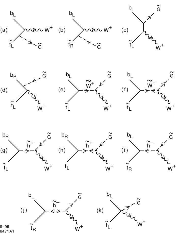
Figure 1: Feynman diagrams for the process ${\widetilde{t}_{1}}\to bW{\widetilde{G}}$. All diagrams are drawn in terms of 2-component fermion notation. $\tilde{G}$ denotes the Goldstino. The label on the $\widetilde{W}$/$\widetilde{h}$ internal lines labels the vertex with which the chargino couples to the top quark.

It is useful to think about building up the complete amplitude for the stop decay by successively considering a number of limiting cases. In Figure 1, we have drawn the diagrams using a basis of weak interaction eigenstates.

The first property to be derived from these amplitudes is the stop decay rate. It is always an issue when an NLSP decays to the gravitino whether the decay is prompt on the times scales of particle physics, or whether the NLSP travels a measureable distance from the production vertex before decaying. Taking into account the 3-body phase space and the fact that the amplitude is proportional to $1/F$, we might roughly estimate the decay amplitude as

$$\Gamma(\widetilde{t}_{1})\sim{\alpha_{w}(m-m_{W})^{7}\over 1028\pi^{2}m_{W}^{2}F^{2}}\ ,$$ (10)

where $\alpha_{w}=g^{2}_{2}/4\pi$ is the weak-interaction coupling constant. By this estimate, a value of $\sqrt{F}$ smaller than 100 TeV would give a prompt decay, with $c\tau<1$ cm.

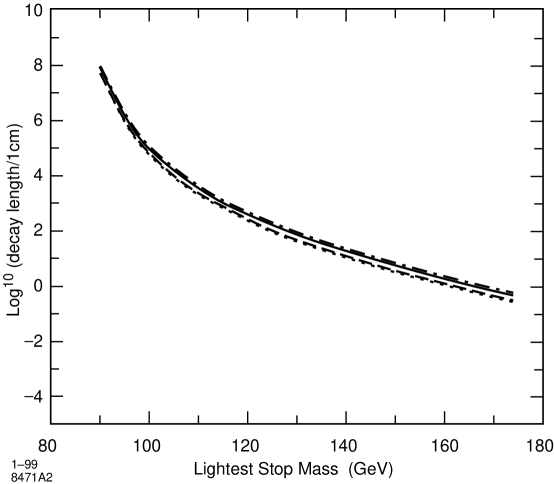
Figure 2: Decay length for the lightest scalar top quark $\tilde{t}_{1}$ as a function of its mass in four different scenarios. The parameters $\sqrt{F}=30$ TeV, $\tan\beta=1.0$, $m_{\tilde{b}_{L}}=300$ GeV, and $\sin{\theta_{t}}=-0.8$ are assumed in all four scenarios.

In Figure 2 we show the result of a complete calculation of the decay rate in the four scenarios listed at the end of Section 2. In all four cases, we have chosen the parameter values $\sqrt{F}=30$ TeV, $\tan\beta=1.0$, $m_{\tilde{b}_{L}}=300$ GeV, and $\sin{\theta_{t}}=-0.8$. The complete calculation reproduces the steep dependence on the stop mass $m$ which is present in (10). and shows that the normalization is roughly correct. Since $\Gamma$ varies as the fourth power of $\sqrt{F}$, one can arrange for a short decay length by making $\sqrt{F}$ sufficiently low. For $m\sim 160$ GeV, the choice $\sqrt{F}=30$ leads to a decay length $c\tau$ of about 1 cm. We have found that the decay length is quite insensitive to all of the other relevant parameters. The variation between scenarios or within a given scenario is less than a factor of 2. From here on, we will analyze the $\widetilde{t}_{1}$ decay as if it were prompt. But it is clear from the figure that, if $\sqrt{F}$ is as low as 30 TeV, stop decays will be identifiable by their displaced vertices in addition to the kinematic signatures discussed in this paper.

The final state of the three-body stop decay is essentially the same as ordinary top decay, since the stop produces a $b$ jet, a $W$ boson, and an unobservable $\widetilde{G}$. How, then, can we distinguish the $t\overline{t}$ and $\widetilde{t}_{1}\widetilde{\overline{t}}_{1}$ production processes? The most straightforward way to approach this problem is to analyze the observable mass distributions of $t$ and $\widetilde{t}_{1}$ decay products. If we could completely reconstruct the $W$ boson, the invariant mass of the $bW$ system would peak sharply at $m_{t}$ in the case of $t$ decay, and would have a more extended distribution below the stop mass $m$ in the case of $\widetilde{t}_{1}$ decay. However, in the observation of top events at the Tevatron, the analysis cannot be so clean. Events from $t\overline{t}$ production are typically observed in the final state in which one $W$ decays hadronically and the second decays to $\ell\nu$. Then the final state contains an unobserved neutrino. If there is only this one missing particle, the event can be reconstructed. But the events with $\widetilde{t}_{1}$ contain two more missing particles, the $\widetilde{G}$s, which potentially confuse the analysis.

Fortunately, it is possible to discriminate $t$ from $\widetilde{t}_{1}$ events by studying the invariant mass distribution of the directly observable $b$ and lepton decay products. For top decays, the distribution in the $b$-lepton invariant mass $m(eb)$ (quoted, for simplicity, for $m_{b}=0$) takes the form

$${1\over\Gamma}{d\Gamma\over dm(eb)}={12m(eb)\over 2(1-m_{W}^{2}/m_{t}^{2})(2+m_{W}^{2}/m_{t}^{2})}(1-y)\bigl{(}1-y+{m_{t}^{2}\over 2m_{W}^{2}}y\bigr{)}\ ,$$ (11)

where $y=m^{2}(eb)/(m_{t}^{2}-m_{W}^{2})$. As is shown in Figure 3, this distribution extends from $m(eb)=m_{b}$ to a kinematic endpoint at $m(eb)=155$ GeV, and peaks toward its high end, at about $m(eb)=120$ GeV. On the other hand, in $\widetilde{t}_{1}$ decay, not only does the $m(eb)$ distribution have a lower endpoint value, reflecting the value of $m<m_{t}$, but it also peaks toward the low end of its range. Figure 3 shows two typical distributions of $m(eb)$, corresponding to stop masses of 130 and 170 GeV. The corresponding distributions of the $b$-$W$ invariant mass $m(bW)$ are also shown for comparison.

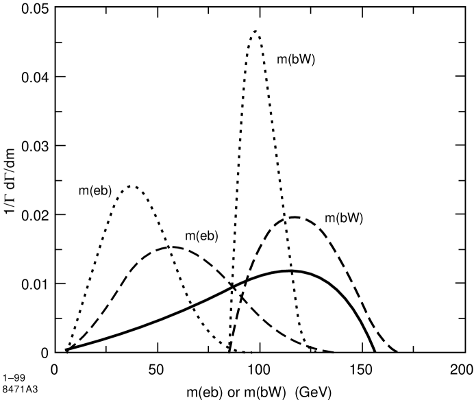
Figure 3: Typical $eb$ and $Wb$ invariant mass distributions for $\widetilde{t}_{1}$ decay. The distributions are shown at two different assumed $\widetilde{t}_{1}$ masses, $m_{\tilde{t}_{1}}=130$ (dotted lines) and 170 GeV (dashed lines), under the scenario (1). The other parameters are chosen as $\tan\beta=1.0$, $m_{\tilde{b}_{L}}=300$ GeV, and $\sin{\theta_{t}}=-0.8$. The solid line shows, for comparison, the $m_{eb}$ spectrum for the standard top quark decay.

A remarkable feature of Figure 3 is that the $m(eb)$ distributions from top and stop decay remain distinctly different even in the limit in which the stop mass $m$ approaches $m_{t}$. Naively, one might imagine that the stop decay diagrams with top quark poles, (a) and (b) in Figure 1, would dominate in this limit and cause the stop decay to resemble top decay. Instead, we find that the top pole diagrams have no special importance in this limit. If $E_{G}$ is the $\widetilde{G}$ energy, the top quark pole gives an energy denominator $1/E_{G}$, but this is cancelled by a $\widetilde{G}$ emission vertex proportional to $(E_{G})^{3/2}$.

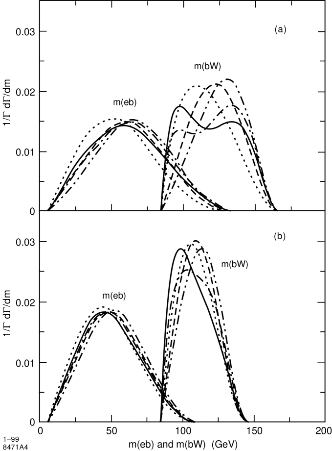
Figure 4: Invariant mass spectra under different scenarios at the two mass values $m_{\tilde{t}_{1}}$: (a)$m_{\tilde{t}_{1}}=170$ GeV, (b) $m_{\tilde{t}_{1}}=150$ GeV. For each case, the parameters are: solid line: scenario (1), $\sin{\theta_{t}}=0.0$, $\tan\beta=1.0$, $m_{\tilde{b}_{L}}=300$ GeV; dotted line: scenario (2), $\sin{\theta_{t}}=-0.8$, $\tan\beta=1.0$, $m_{\tilde{b}_{L}}=300$ GeV; dashed line: scenario (3), $\sin{\theta_{t}}=0.9$, $\tan\beta=50.0$, $m_{\tilde{b}_{L}}=200$ GeV; dot-dashed line: scenario (3), $\sin{\theta_{t}}=0.0$, $\tan\beta=1.0$, $m_{\tilde{b}_{L}}=300$ GeV; long-dashed line: scenario (4), $\sin{\theta_{t}}=0.4$, $\tan\beta=8.0$, $m_{\tilde{b}_{L}}=200$ GeV.

In Figure 4, we show the variation of the the distribution of $m(eb)$ and $m(bW)$ according to the choice of the supersymmetry parameters. The five curves in each group correspond specific parameter choices in the four scenarios listed at the end of Section 2, plus an additional choice in scenario (3) corresponding to the case of a pure $\widetilde{t}_{L}$ ($\theta_{t}=0$). The distributions for a given value of $m$ are remarkably similar. Presumably, the shape of these distributions is determined more by general kinematic constraints than by the details of the decay amplitudes. The only exception to this rule that we have found comes in the case where the $\widetilde{t}_{1}$ is dominantly $\widetilde{t}_{L}$ and the $\widetilde{w}$ exchange process is especially important.

From these results, we believe that the $\widetilde{t}_{1}$ production process can be identified by measuring the distribution of $m(eb)$ in events that pass the top quark selection criteria. The mass of the $\widetilde{t}_{1}$ can be estimated from this distribution to about 5 GeV without further knowledge of the other supersymmetry parameters.

4 Longitudinal $W$ polarization

One of the characteristic predictions of the standard model for top decay is that the final-state $W$ bosons should be highly longitudinally polarized. Define the degree of longitudinal polarization by

$$r={\Gamma(W_{0})\over\Gamma(\mbox{all})}\ .$$ (12)

Then the leading-order prediction for this polarization in top decay is

$$r_{t}={1\over 1+2m_{W}^{2}/m_{t}^{2}}\approx 0.71\ .$$ (13)

We have seen already that the configuration of the final $bW^{+}$ system in stop decay is quite different from that in top decay. Thus, it would seem likely that the longitudinal $W$ polarization would also deviate from the characteristic values for top. We will show that the value of $r$ in stop decay typically differs significantly from (13), in a manner that gives information about the underlying supersymmetry model.

The measurement of the polarization $r$ at the Tevatron has been studied using the technique of reconstructing the $W$ decay angle in single-lepton events from the lepton and neutrino four-vectors [14, 15]. An accuracy of $\pm 0.03$ should be achieved in the upcoming Run II. This technique, however, cannot be used for stop events, since the missing momentum includes the $\tilde{G}$’s as well as the neutrino. However, one can also measure the longitudinal $W$ polarization from the $W$ decay angle determined by using the four-vectors of the two jets assigned to the hadronic $W$ in the event reconstruction. It is not necessary to distinguish the quark from the antiquark to determine the degree of longitudinal polarization.

What value of $r$ should be found for light stop pair production? In Figures 5 and 6, we plot the value of $r$ in the four scenarios listed at the end of Section 2, for representative values of the parameters, as a function of the stop mass. We see that the value of $r$ is typically lower than the top quark value (13), that it has a slow dependence on the value of the stop mass $m$, and that it can depend significantly on the stop mixing angle $\theta_{t}$.

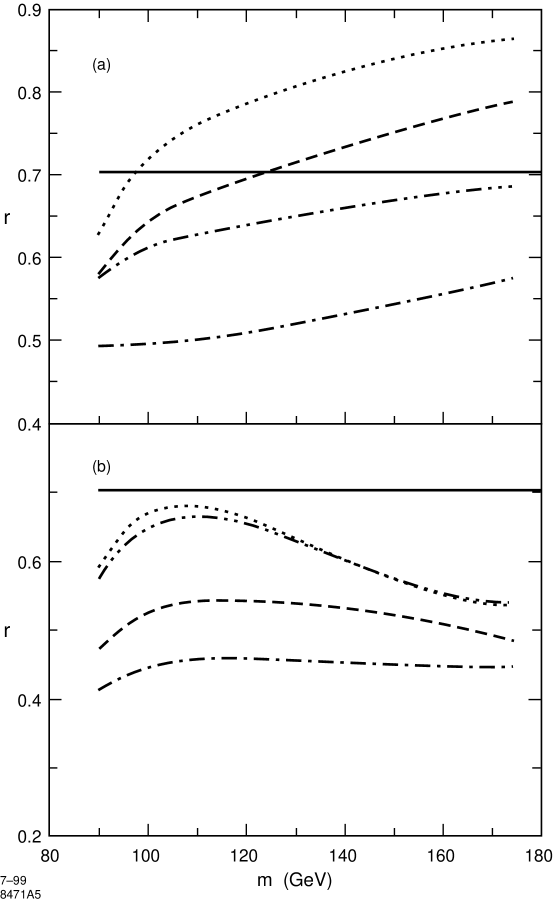
Figure 5: Longitudinal W production ratio for the stop $\tilde{t}_{1}$ decay as a function of $m_{\widetilde{t}_{1}}$ under different scenarios. The dot-dash, dotted, dashed, and dot-dot-dash lines refer, respectively, to the chargino scenarios (1), (2), (3), (4) given at the end of Section 2. The two figures show (a) $\tilde{t}_{R}$-like cases with $sin{\theta_{t}}=-0.8$, $tan\beta=1.0$, and $m_{\tilde{b}_{L}}=300$ GeV. (b) pure $\tilde{t}_{L}$-like cases with $sin{\theta_{t}}=0.0$, $tan\beta=1.0$, and $m_{\tilde{b}_{L}}=300$ GeV.

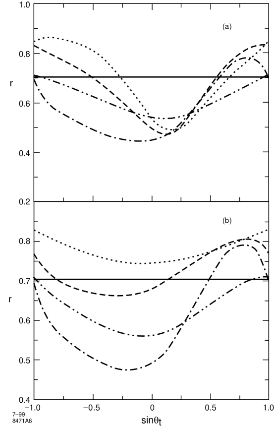
Figure 6: Longitudinal W production ratio for the stop $\tilde{t}_{1}$ decay as a function of $sin{\theta_{t}}$ under different scenarios. The dot-dash, dotted, dashed, and dot-dot-dash lines refer, respectively, to the chargino scenarios (1), (2), (3), (4) given at the end of Section 2. The two figures show the dependence for (a) $m_{\tilde{t}_{1}}=170$ GeV, $tan\beta=1.0$, and $m_{\tilde{b}_{L}}=300$ GeV. (b) $m_{\tilde{t}_{1}}=170$ GeV, $tan\beta=50.0$, and $m_{\tilde{b}_{L}}=300$ GeV.

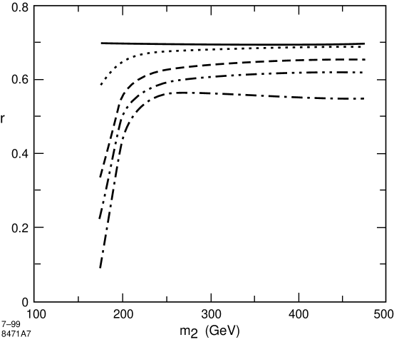
Figure 7: Longitudinal W production ratio for the stop $\tilde{t}_{1}$ decay as a function of the soft breaking mass of SU(2) gaugino. The four curves correspond to $\sin\theta_{t}=$ -0.98, -0.8, -0.6, 0.0. The other parameters are chosen to be $m_{\tilde{t}_{1}}=170$ GeV, $tan\beta=1.0$, $\mu=1000$ GeV, and $m_{\tilde{b}_{L}}=300$ GeV.

The variation of $r$ arises from the competition between the diagrams in Figure 1 in which the Goldstino is radiated from the $t$ and $b$ legs and those in which the Goldstino is radiated from the $W$. To understand this, it is useful to think about the limiting cases in which each intermediate propagator goes on shell. In the case in which the top quark goes on shell in diagrams a,b of Figure 1, the $W$ polarization has the same vlaue (13) as that for top decay. In the case in which the $\widetilde{b}$ goes on shell, we have the process $\widetilde{t}\to\widetilde{b}W^{+}$, for which also $r=1/(1+2m_{W}^{2}/m_{t}^{2})$. However, the third case in which the $\widetilde{\chi}^{+}$ goes on shell can give a very different result. In the limit in which the $\widetilde{\chi}^{+}$ is pure gaugino, we have the subprocess $\widetilde{w}^{+}\to\widetilde{G}W^{+}$, which leads to purely transversely polarized $W$ bosons. More generally, for the process $\widetilde{\chi}^{+}_{1}\to\widetilde{G}W^{+}$ on shell, we have

$$r={|V_{+12}|^{2}+|V_{-12}|^{2}\over 2(|V_{+11}|^{2}+|V_{-11}|^{2})+|V_{+12}|^{2}+|V_{-12}|^{2}}\ ,$$ (14)

where $V_{+}$, $V_{-}$ are the matrices defined in (7). These individual components vary in importance as the masses on the intermediate lines are varied. The role of the chargino diagrams in producing a low value of $r$ is shown clearly in Figure 7. Here we plot the value of $r$ as a function of the supersymmetry-breaking $SU(2)$ gaugino mass $m_{2}$ and observe that $r$ moves to a higher asymptotic value as the gaugino is decoupled.

Beyond this observation, though, the dependence of $r$ on the underlying parameters is not simple. As we have seen in the previous section, it is never true that one particular subprocess comes almost onto mass shell and dominates the stop decay. This feature of the stop decay, which was an advantage in the previous section, here provides a barrier to finding quantitative relation between a measured value of $r$ and the underlying parameter set. On the other hand, it is interesting that almost every scenario predicts a value of $r$ substantially different from the Standard Model value for top decay.

5 Conclusions

In this paper, we have discussed the phenomenology of light stop decay through the process $\widetilde{t}\to W^{+}b\widetilde{G}$. We have shown that this process can be distinguished from $t$ decay through the characteristic shape of the $b\ell$ mass distribution. We have shown also that the fraction of longitudinal polarization of the $W^{+}$ in $\widetilde{t}$ decays can vary significantly from the prediction (13) for $t$. Since these two observables are available at the Tevatron collider, it should be possible there to exclude or confirm this unusual scenario for the realization of supersymmetry.

ACKNOWLEDGEMENTS

We are grateful to Scott Thomas for suggesting this problem, to Regina Demina, for encouragement and discussions on stop experimentation, and to JoAnne Hewett, for helpful advice. This work was supported by the Department of Energy under contract DE–AC03–76SF00515.

References

- [1] H. P. Nilles, Phys. Repts. 110, 1 (1984).
- [2] H.E. Haber and G. L. Kane, Phys. Rep. 117 75 (1985).
- [3] S. Dawson, hep-ph/9712464, in Supersymmetry, Supergravity, and Supercolliders: Proceedings of TASI-97, J. Bagger, ed. (World Scientific, Singapore, 1999).
- [4] R. Arnowitt, P. Nath, and A. H. Chamseddine, Applied N=1 Supergravity (World Scientific, Singapore, 1984).
- [5] M. Dine, A. E. Nelson and Y. Shirman, hep-ph/9408384, Phys. Rev.D51, 1362 (1995); M. Dine, A. E. Nelson, Y. Nir and Y. Shirman, hep-ph/950378, Phys. Rev. D53, 2658 (1996).
- [6] S. Ambrosanio, G. L. Kane, G. D. Kribs and S. P. Martin, hep-ph/9605398, Phys.Rev. D54, 5395 (1996); S. Ambrosanio, G. D. Kribs and S. P. Martin, hep-ph/9703211, Phys.Rev. D56, 1761 (1997).
- [7] S. Dimopoulos, M. Dine, S. Raby and S. Thomas, hep-ph/9601367, Phys. Rev. Lett.76, 3494 (1996); S. Dimopoulos, S. Thomas and J. D. Wells, hep-ph/9609434, Nucl.Phys. B488, 39 (1997).
- [8] S. Ambrosanio, G. D. Kribs, and S. P. Martin, hep-ph/9710217, Nucl. Phys. B516, 55 (1998).
- [9] S. Thomas, personal communication; S. Mrenna, personal communication.
- [10] T. Kon and T. Nonaka, hep-ph/9404230, hep-ph/9405327, Phys. Rev. D50, 6005 (1994).
- [11] J. L. Lopez, D. V. Nanopoulos, and A. Zichichi, hep-ph/9406254, Mod.Phys.Lett. A10, 2289 (1995).
- [12] G. L. Kane, G. A. Ladinsky, and C.-P. Yuan, Phys. Rev. D45, 124 (1992); G. A. Ladinsky, Phys. Rev. D46, 3789 (1992), E D47, 3086 (1993).
- [13] P. Fayet, Phys. Lett.B70, 461 (1977).
- [14] T. Affolder, et al. [CDF Collaboration], hep-ex/9909042.
- [15] R. Blair, et al. (CDF II Collaboration), The CDF II Detector Technical Design Report. (Fermilab, 1996); T. Affolder, et al. (CDF Collaboration), hep-ex/9909042.