The Two-Loop Static Potential

Abstract

In quantum chromodynamics (QCD), the binding energy of an infinitely heavy quark–antiquark pair in a color singlet state can be calculated as a function of the distance. We investigate this static potential of QCD perturbatively and calculate the full two-loop coefficient, correcting an earlier result. Beyond this order, the perturbative expansion breaks down.

1 Introduction

The static potential of quantum chromodynamics (QCD) is subject to theoretical investigations since more than twenty years. Being the non–abelian analogue of the well–known Coulomb potential of quantum electrodynamics (QED), this interaction energy of an infinitely heavy quark–antiquark pair is a fundamental concept which is expected to play a key role in the understanding of quark confinement. Moreover, the static potential is a major ingredient in the description of non–relativistically bound systems like quarkonia, and it is of importance in many other areas, such as quark mass definitions and quark production at threshold.

It is expected that the static potential consists of two terms: a Coulomb–like term at short distances, which is calculable with perturbative methods, and a long–distance term responsible for confinement. Even though a perturbative analysis is not suited to give the full potential, such a calculation proves very useful. The short–distance part of the potential can be utilized as a refined starting point for the construction of potential models (which have been rather successful in the past for the description of quarkonia), or it could describe very heavy systems (like $\bar{t}t$) to good accuracy. Furthermore, it can be compared to the results of numerical calculations in lattice gauge theory. It is natural to define the QCD coupling constant with help of the potential as $V(r)=-\frac{4}{3}\frac{\alpha_{\scriptscriptstyle V}(1/r)}{r}$, the so-called V–scheme, using a physical quantity in contrast to the usual coupling definition in the ${\overline{{\rm MS}}}$ scheme. In lattice calculations $\alpha_{\scriptscriptstyle V}$ is regarded as as the ’better’ expansion parameter [1]. For these reasons, and to get a more precise determination of $\alpha_{{}\over{\rm MS}}$ from the lattice, the relation between the two couplings has to be known.

A first determination of the static potential in (massless) QCD has been performed by L. Susskind in the context of a lecture about lattice gauge theory [2]. In order to demonstrate asymptotic freedom in Yang–Mills theory, he calculated the one-loop pole terms using a Wilson–loop formula for the potential, and re-derived the first coefficient of the renormalization group Beta function. This work was extended by other groups quite soon, who then added fermionic contributions [3] and two-loop pole terms [4] to the potential, as well as examined the structure of higher–order corrections qualitatively [5]. Recently, the perturbative static potential has received new interest, in particular due to its application in top–quark production at threshold [6], a process that comes within experimental reach in the near future. A complete two-loop calculation for the static potential was performed in ref. [7]. Such an important result clearly needs confirmation. This is one of the motivations of our work on the two-loop potential [8, 9]. More recently, the effect of fermion masses was considered on the two-loop level in ref. [10].

2 Definition and Expansion

The static potential is defined in a manifestly gauge invariant way via the vacuum expectation value of a Wilson loop [4, 11],

$$\mbox{}V(r)=-\lim_{T\rightarrow\infty}\frac{1}{T}\,\ln\left\langle\vphantom{A^{b}_{\mu}}{\cal W}_{\Gamma}\right\rangle\;,$$ (1)

$$\mbox{}{\cal W}_{\Gamma}=\widetilde{\rm tr}\,{\cal P}\exp\left(ig\oint_{\Gamma}dx_{\mu}A_{\mu}\right)\;.$$ (2)

Here, $\Gamma$ is taken as a rectangular loop with time extension $T$ and spatial extension $r$. The gauge fields $A_{\mu}$ are path-ordered along the loop, while the color trace is normalized according to $\widetilde{\rm tr}(..)={\rm tr}(..)/{\rm tr}1\!\!1\,$.

In a perturbative analysis it can be shown that, at least to the order needed here, all contributions to eq. (1) containing connections to the spatial components of the gauge fields $A_{i}(\mbox{\boldmath$r$},\pm T/2)$ vanish in the limit of large time extension $T$. Hence, the definition can be reduced to

$$V_{\rm pert}=-\lim_{T\rightarrow\infty}\frac{1}{T}\,\ln\left\langle\vphantom{A^{b}_{\mu}}\widetilde{\rm tr}\,{\cal T}\exp\left(\int_{x}\!J_{\mu}^{a}A_{\mu}^{a}\right)\right\rangle\;,$$ (3)

where ${\cal T}$ means time ordering and the static sources separated by the distance $r=|\mbox{\boldmath$r$}-\mbox{\boldmath$r$}\,^{\prime}|$ are given by

$$J_{\mu}^{a}(x)=ig\,\delta_{\mu 0}\,T^{a}\,\left[\,\delta(\mbox{\boldmath$x$}-\mbox{\boldmath$r$})-\delta(\mbox{\boldmath$x$}-\mbox{\boldmath$r$}\,^{\prime})\,\right]\,\;,$$ (4)

where $T^{a}$ are the generators in the fundamental representation. In the case of QCD the gauge group is $SU(3)$. The results will be presented for an arbitrary compact semi-simple Lie group with structure constants defined by the Lie algebra $[T^{a},T^{b}]=if^{abc}T^{c}$. The Casimir operators of the fundamental and adjoint representation are $T^{a}T^{a}=C_{F}$ and $f^{acd}f^{bcd}=C_{A}\delta^{ab}$. $tr(T^{a}T^{b})=T_{F}\delta^{ab}$ is the trace normalization, while $n_{f}$ denotes the number of massless quarks.

Expanding the expression in eq. (3) perturbatively, one encounters in addition to the usual Feynman rules the source–gluon vertex $ig\delta_{\mu 0}T^{a}$, with an additional minus sign for the antisource. Furthermore, the time–ordering prescription generates step functions, which can be viewed as source propagators, analogous to the heavy–quark effective theory (HQET).

Concerning the generation of the complete set of Feynman diagrams contributing to the two–loop static potential, there are some subtleties connected with the logarithm in the definition (3). All this is explained in detail in [4, 7, 9], so we only list the relevant exchange diagrams here (see fig.1).

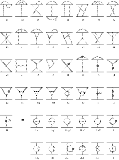
Figure 1: Classes of two–loop diagrams contributing to the static potential. Double, wiggly, dotted and solid lines denote source, gluon, ghost and (light) fermion propagators, respectively. A blob on a gluon line stands for one–loop self–energy corrections.

3 Method

Turning to the purely technical side of the work documented here, only part of the Feynman diagrams to be considered, namely the pure self-energy contributions to the static potential, are amenable to standard calculation methods [12, 13, 14, 15]. For the others, essentially being two–point functions also, but involving non–covariant propagators, the standard methods need to be generalized. We have developed a general strategy to deal with these expressions, which is based on a purely algebraic reduction to a minimal set of integrals [9].

The method employed can be briefly summarized as follows:

• Working in momentum space, all dimensionally regulated (tensor-) integrals are reduced to pure propagator integrals by a generalization of the method of $T$–operators [14]. The resulting expressions are then mapped to a minimal set of five scalar integrals by means of recurrence relations, again generalizing [14] as well as [12] to the case including static (non-covariant) propagators. These two steps have been implemented into a FORM package. Thus, we constructed our method to be complementary to the calculation in ref. [7], assuring a truly independent check of the result presented therein. At this stage, one obtains analytic coefficient functions (depending on the generic space–time dimension $D$ as well as on the color factors and the bare coupling), multiplying each of the basic integrals.

• The basic scalar integrals are then solved analytically. Expanding the result around $D=4$ (which is done in both MAPLE and Mathematica considering the complexity of the expressions), renormalizing and Fourier transforming back to coordinate space, one obtains the final results presented below.

Important checks of the calculation include

• gauge independence of appropriate classes of diagrams,

• confirmation of cancelation of infrared divergences,

• correct renormalization properties.

4 Result and Discussion

We obtain, as our final result for the two-loop static potential in coordinate space,

$$V(r)=-C_{F}\,\frac{\alpha_{\scriptscriptstyle V}(1/r^{2})}{r}\;,$$ (5)

with

$$\mbox{}\alpha_{\scriptscriptstyle V}(1/r^{2})\;=\;\alpha_{{}\over{\rm MS}}\left\{\vphantom{\int}\right.1+\frac{\alpha_{{}\over{\rm MS}}}{4\pi}\,(a_{1}+\beta_{0}L)$$

$$\mbox{}{}+\frac{\alpha_{{}\over{\rm MS}}^{2}}{16\pi^{2}}\left(a_{2}+\beta_{0}^{2}(L^{2}+\frac{\pi^{2}}{3})+(\beta_{1}+2\beta_{0}a_{1})L\right)$$

$$\mbox{}{}+{\cal O}(\alpha_{{}\over{\rm MS}}^{3})\left.\vphantom{\int}\right\}\;,$$ (6)

where $L=2\ln(\bar{\mu}re^{\gamma})$ and $\alpha_{{}\over{\rm MS}}=\alpha_{{}\over{\rm MS}}(\bar{\mu}^{2})$. The first two terms of the beta function are given by $\beta_{0}=\frac{11}{3}\,C_{A}-\frac{4}{3}\,T_{F}n_{f}$ and $\beta_{1}=\frac{34}{3}\,C_{A}^{2}-4C_{F}T_{F}n_{f}-\frac{20}{3}\,C_{A}T_{F}n_{f}$. The one- and two-loop constants read

$$a_{1} = \frac{31}{9}\,C_{A}-\frac{20}{9}\,T_{F}n_{f}\;,$$ (7)

$$a_{2} = \left(\frac{4343}{162}+4\pi^{2}-\frac{\pi^{4}}{4}+\frac{22}{3}\zeta(3)\right)C_{A}^{2}$$ (8)

$${}-\left(\frac{55}{3}-16\zeta(3)\right)C_{F}T_{F}n_{f}+\frac{400}{81}\,T_{F}^{2}n_{f}^{2}$$

$${}-\left(\frac{1798}{81}+\frac{56}{3}\,\zeta(3)\right)C_{A}T_{F}n_{f}\;,$$

respectively. As it has to be, the coefficients prove to be gauge independent. Comparing our two-loop result for $a_{2}$ with [7], we find a discrepancy of $2\pi^{2}$ in the pure Yang–Mills term ($\propto C_{A}^{2}$). This amounts to a $30\%$ decrease of $a_{2}$ for the case of $n_{f}=0$, and a $50\%$ decrease for $n_{f}=5$ (for $SU(3)$), which is the case needed for $t\bar{t}$ threshold investigations. This difference can be traced back to a specific set of diagrams, and it is clarified with the author of ref. [7] .

There are now numerous concepts for a ’renormalization group improvement’, i.e. for an ’optimal’ choice of the ${\overline{{\rm MS}}}$ scale parameter $\bar{\mu}$ in order to reduce large logarithmic corrections. Examples include the ’natural choice’ $\bar{\mu}=e^{-\gamma}/r$ and the choice $\bar{\mu}=\exp(-\gamma-a_{1}/2\beta_{0})/r$, which eliminates the one-loop coefficient completely. Due to this freedom, it is not very illuminating to present plots of the coordinate space potential. A general feature is that, at increasing distance, the large two-loop coefficient begins to dominate quite soon, even causing the potential to decrease again above some $r_{\rm crit}$, to signal that the perturbative approach can be followed up to this critical distance at most. For a discussion of a variety of scale choices we refer to ref. [7]. The smaller coefficient $a_{2}$ found in our calculation does not change the plots presented there qualitatively. The reason is that the term $\frac{\pi^{2}}{3}\beta_{0}^{2}$, which shows up as a result of the Fourier transform, is of the same order as $a_{2}$.

Concerning the convergence of the series (4), let us give some numbers. For SU(3), $T_{F}={\scriptstyle\frac{1}{2}\,}$ and the ’natural’ scale choice, we have

$$\alpha_{\scriptscriptstyle V} = \alpha_{{}\over{\rm MS}}\left\{\vphantom{\int}\right.1+\frac{\alpha_{{}\over{\rm MS}}}{\pi}\,(2.6-0.3n_{f})$$ (9)

$${}+\frac{\alpha_{{}\over{\rm MS}}^{2}}{\pi^{2}}\,(53.4-7.2n_{f}+0.2n_{f}^{2})+..\left.\vphantom{\int}\right\}\;.$$

In ref. [7], the first number in the two-loop term was $64.5$. Apparently the convergence properties do still not look very promising.

A comparison with four–dimensional quenched lattice results is given in ref. [16]. There, it is concluded that the perturbative potential already fails to describe the slope of the lattice potential at the smallest distances that are numerically tractable, hence invalidating the possibility to match the two potentials at small distances.

Summarizing, we have re-calculated the two–loop static potential by a method complementary to the approach in [7]. We have developed an algorithm which enables us to work in general covariant gauges throughout. Confirming the fermionic contributions to the two–loop coefficient $a_{2}$, we find a substantial deviation in the pure gluonic part of $a_{2}$. The source of the discrepancy could be identified. The bad convergence of the perturbative series does not improve considerably taking into account the new value of $a_{2}$. Hence, the use of a physical coupling, defined by the potential, as expansion parameter seems to be disfavored. Further studies are clearly needed to clarify the role of higher–order corrections. There has always been discussion about whether the perturbative Wilson–loop formula is a good definition of the static potential, which can be questioned due to possible infrared divergences in higher orders [5]. A redefinition was proposed recently [17], which becomes effective at the three-loop level.

References

- [1] G.P. Lepage and P.B. Mackenzie, Phys. Rev. D 48 (1993) 2250.
- [2] L. Susskind, Coarse grained QCD in R. Balian and C.H. Llewellyn Smith (eds.), Weak and electromagnetic interactions at high energy (North Holland, Amsterdam, 1977).
- [3] A. Billoire, Phys. Lett. B 92 (1980) 343.
- [4] W. Fischler, Nucl. Phys. B 129 (1977) 157.
- [5] T. Appelquist, M. Dine and I.J. Muzinich, Phys. Lett. B 69 (1977) 231; Phys. Rev. D 17 (1978) 2074.
- [6] for a recent review, see A.H. Hoang and T. Teubner, preprint CERN-TH-99-59.
- [7] M. Peter, Phys. Rev. Lett. 78 (1997) 602; Nucl. Phys. B 501 (1997) 471.
- [8] Y. Schröder, Phys. Lett. B 447 (1999) 321.
- [9] Y. Schröder, Ph. D. thesis, DESY-THESIS-1999-021.
- [10] M. Melles, Phys. Rev. D 58 (1998) 114004.
- [11] E. Eichten and F.L. Feinberg, Phys. Rev. Lett. 43 (1979) 1205; Phys. Rev. D 23 (1981) 2724.
- [12] K.G. Chetyrkin and F.V. Tkachov, Nucl. Phys. B 192 (1981) 159.
- [13] A.I. Davydychev, Phys. Lett. B 263 (1991) 107.
- [14] O.V. Tarasov, Phys. Rev. D 54 (1996) 6479.
- [15] O.V. Tarasov, Nucl. Phys. B 502 (1997) 455.
- [16] G.S. Bali, Phys. Lett. B 460 (1999) 170.
- [17] N. Brambilla, A. Pineda, J. Soto and A. Vairo, preprint CERN-TH-99-61; see also these proceedings.