Neutralino Relic Density in a Universe with a non-vanishing Cosmological Constant

Abstract

We discuss the relic density of the lightest of the supersymmetric particles in view of new cosmological data, which favour the concept of an accelerating Universe with a non-vanishing cosmological constant. Recent astrophysical observations provide us with very precise values of the relevant cosmological parameters. Certain of these parameters have direct implications on particle physics, e.g., the value of matter density, which in conjunction with electroweak precision data put severe constraints on the supersymmetry breaking scale. In the context of the Constrained Minimal Supersymmetric Standard Model (CMSSM) such limits read as: $M_{1/2}\simeq 300\;\mathrm{GeV}-340\;\mathrm{GeV}$, $m_{0}\simeq 80\;\mathrm{GeV}-130\;\mathrm{GeV}$. Within the context of the CMSSM a way to avoid these constraints is either to go to the large $\tan\beta$ and $\mu>0$ region, or make ${\tilde{\tau}}_{R}$, the next to lightest supersymmetric particle (LSP), be almost degenerate in mass with LSP.

I Introduction

During the last few years the knowledge of the cosmological parameters has started entering an era of high precision with far reaching consequences not only for cosmology, but for particle physics as well. The cosmic microwave background temperature is accurately known, $T_{0}=2.7277\pm 0.002\;^{0}\mathrm{K}$, the Hubble parameter is determined with a relatively small error, $H_{0}=65\pm 5\;\mathrm{Km/sec/Mpc}$, the baryonic mass density is precisely determined by big-bang nucleosynthesis, $\Omega_{\mathrm{B}}h_{0}^{2}=0.019\pm 0.001$, while the determination of the age of the Universe from the oldest stars, as well as other sources, yield $t_{U}=14\pm 1.5\;\mathrm{Gyr}$ [1]. Very recent observations of type Ia supernovae (SNIa), as well as measurements of the anisotropy of the Cosmic Background Radiation (CBR) provide additional information favouring an almost flat and accelerating Universe, where the acceleration mainly is driven by a non-vanishing cosmological constant [2, 3, 4].

There is a growing consensus that the anisotropy of the CBR offers the best way to determine the curvature of the Universe and hence the total matter-energy density $\Omega_{0}$ [1]. The data are consistent with a flat Universe, ${\Omega}_{0}=1.0\pm 0.2$, while we are confident that the radiation component of the matter-energy density, that is the contribution from CBR and/or ultra relativistic neutrinos, is very small [1, 2]. Therefore the present matter-energy density can be decomposed principally into matter density $\Omega_{\mathrm{M}}$ and vacuum energy $\Omega_{\Lambda}$:

$$\Omega_{0}=\Omega_{\mathrm{M}}+\Omega_{\Lambda}\,.$$ (1)

There is also supporting evidence, coming from many independent astrophysical observations, that the matter density weighs $\Omega_{\mathrm{M}}=0.4\pm 0.1$ (see for instance Ref. [1] and references therein). The $\Omega_{\mathrm{M}},\;\Omega_{\Lambda}$ values are then restricted by the age of the Universe and by the value of the Hubble parameter through

$$t_{U}={\frac{1}{H_{0}}}\;{\int_{0}^{1}}\;dy\;\sqrt{y\over{{\Omega}_{\mathrm{M}}(1-y)+{\Omega}_{\Lambda}(y^{3}-y)+y}}\,.$$ (2)

The constraints stemming from Eq. (2) are however less restrictive than those coming from the supernovae SNIa data. Recently two groups, the Supernova Cosmology Project [3] and the High-$z$ Supernova Search Team [4], using different methods of analysis, each found evidence for accelerated expansion, driven by a vacuum energy contribution:

$$\Omega_{\Lambda}={4\over{3}}\Omega_{\mathrm{M}}+{1\over{3}}\pm{1\over{6}}\,.$$ (3)

So, for $\Omega_{\mathrm{M}}=0.4\pm 0.1$ this relation implies that the vacuum energy is non-vanishing, $\Omega_{\Lambda}=0.85\pm 0.2$, a value which is compatible with a flat Universe, as the anisotropy of CBR measurements indicate. Taking into account the fact that the baryonic contribution to the matter density is small, ${\Omega}_{\mathrm{B}}=0.05\pm 0.005$, the values for matter energy density $\Omega_{\mathrm{M}}$ result to a Cold Dark Matter (CDM) density ${\Omega}_{\mathrm{CDM}}\simeq 0.35\pm 0.1$, which combined with more recent measurements [1, 5] of the scaled Hubble parameter $h_{0}=0.65\pm 0.05$, result to small CDM relic densities:

$$\Omega_{\mathrm{CDM}}\,{h_{0}}^{2}\simeq 0.15\pm 0.07\,.$$ (4)

From measurements of the ratio of the baryonic to total mass in rich clusters, smaller values for the mass density are obtained. This ratio is found to be $\Omega_{\mathrm{B}}/\Omega_{\mathrm{M}}\thickapprox 0.15$ [6, 7] which entails to even tighter limits $\Omega_{\mathrm{CDM}}\,{h_{0}}^{2}=0.12\pm 0.04$ [8].

Such stringent bounds for the CDM relic density affect supersymmetric predictions and may lower the limits of the effective supersymmetry breaking scale, and hence the masses of the supersymmetric particles. In Ref. [9] within the framework of the string inspired no-scale $SU(5)\times U(1)$ supergravity model, by relaxing the cosmological constant, regions of the parameter space compatible with $\Omega_{\mathrm{CDM}}\,{h_{0}}^{2}\thickapprox 0.2$ were delineated, and phenomenological predictions for the sparticle spectrum were given. The relevance of the high precision cosmology to constrained supersymmetry was addressed in Refs. [10, 11]. More recently the CDM relic abundance with non-vanishing cosmological constant, in the framework of the Minimal Supersymmetric Standard Model (MSSM), was shown to put limits on supersymmetric mass spectrum [12]. In fact it was shown that gauginos can be within LHC reach, if the recent cosmological data are used. As stated in Ref. [13] it is worth pointing out that while electroweak (EW) precision data are in perfect agreement with Standard Model (SM) predictions, and hence in agreement with supersymmetric models which are characterized by a large supersymmetry breaking scale ${M}_{\mathrm{SUSY}}$ [14], the data on ${\Omega}_{\mathrm{CDM}}\,{h_{0}}^{2}$ push ${M}_{\mathrm{SUSY}}$ to the opposite direction preferring small values of ${M}_{\mathrm{SUSY}}$. Therefore EW precision data may be hard to reconcile with the assumption that the lightest supersymmetric particle (LSP or $\tilde{\chi}$), is a candidate for CDM [13].

The method to calculate the relic abundance of a Dark Matter (DM) candidate particle in the Universe is outlined in Ref. [15]. In $R$-parity conserving supersymmetric theories the LSP may be a neutralino, which is a good candidate to play the role of DM [16]. Many authors [17, 18, 19, 20, 21, 22, 23, 24, 25, 26, 27, 28, 29, 30, 10, 11, 12, 31, 32, 35, 36] have since calculated the relic neutralino density. In the early works, only the most important neutralino annihilation channels were considered, but later works [27, 28] included all annihilation channels. Also more refined calculations of thermal averages of cross sections were employed, which took into account threshold effects and integration over Breit-Wigner poles [33, 34].

Our study in this paper is based on the CMSSM, which is motivated by Supergravity, assuming universal boundary conditions for the soft supersymmetry breaking parameters, and in which the EW symmetry is radiatively broken [38]. Our strategy of calculating the neutralino relic density follows three steps: First the SUSY particle spectrum and the relevant couplings are generated, according to the supersymmetric scenario mentioned above. Then the thermally averaged cross sections $\left\langle\sigma v\right\rangle$ are calculated in their non-relativistic limit, using analytic expressions. Finally we numerically solve the Boltzmann equation, which governs the evolution of the neutralino relic density, by using very accurate routines able to handle stiff problems of differential equations. Regarding the calculation of the relic density, we solve the Boltzmann equation numerically by finding a proper boundary condition along the lines described in Ref. [26]. This is reminiscent of the WKB approximation; it yields very accurate results and differs from the standard approaches used in most works. We want to emphasize that for the sake of the effectiveness of our computational code we have chosen to use analytic results in order to calculate the amplitudes of the processes contributing to thermally averaged cross section $\left\langle\sigma v\right\rangle$ [27]. The price one pays, is that these analytic results break down in the vicinity of the poles or thresholds of the cross section. However the comparison of our results with those of other studies [24, 28], which treat the problem of poles and thresholds in a more accurate manner by calculating numerically the thermally averaged cross section [33, 34], shows that they are in striking agreement. This occurs, at least, in regions of the parameter space of the CMSSM where this comparison is feasible.

The effect of the coannihilation between the LSP and the next-to-lightest supersymmetric particle (NLSP) is quite important and should be duly taken into account [37, 33, 22, 30, 10]. The importance of coannihilation of the lightest of the neutralinos $\tilde{\chi}$, which in most of the parameter space of the CMSSM is a bino, with $\tilde{\tau}_{R}$ has been pointed out in Refs. [31, 39]. $\tilde{\chi}-\tilde{\tau}_{R}$ coannihilation are of relevance for values of the parameters near the edge where $\tilde{\chi}$ and ${\tilde{\tau}}_{R}$ are almost degenerate in mass. In such regions of the parameter space the results reached using the ordinary methods, in which these effects are neglected, have to be properly modified to correctly account for the effect of the coannihilation.

As a preview of our results:
We have found that within the context of the CMSSM the recent cosmological data, in combination with EW precision measurements, lead to rather tight limits for the relevant supersymmetric breaking parameters $m_{0}$, $M_{1/2}$, provided the next to the LSP particle (${\tilde{\tau}}_{R}$) is not nearly degenerate in mass with the LSP. In this regime the only option to avoid these limits is to move to the large $\tan\beta$ region, where acceptable relic densities can be obtained if the pseudoscalar Higgs mass is approaching twice the mass of the LSP. This case is consistent with $b\rightarrow s\gamma$ and may be of relevance for models in which Yukawa coupling unification is enforced.

In regions of the parameter space in which ${\tilde{\tau}}_{R}$’s mass is close to that of the LSP, where coannihilation processes need be taken into account for the calculation of the actual neutralino relic abundance, such limits can be evaded.

This paper is organized as follows:
In the first section we give the basic formalism and discuss various details of our calculations. In section II and III we discuss the methodology we follow in solving the Boltzmann equation and give details of our numerical computation. In section IV our results for the LSP relic density are presented and regions of the parameter space consistent with the new astrophysical data are delineated. Towards the end of this section a discussion is devoted to the coannihilation effects. Finally we end up with the conclusions. To facilitate the reader the supersymmetric conventions used throughout this paper are presented in the Appendix.

II Supersymmetric relic density

Our aim is to calculate the cosmological relic density of the lightest of the supersymmetric particles, which will be denoted by $\tilde{\chi}$ throughout this paper. This we assume is one of the four neutralinos states. In supersymmetric models with $R$-parity conservation this particle is stable. The cosmological constraints on ${\Omega}_{\mathrm{CDM}}$ discussed previously may impose stringent constraints on its mass, as well as on the masses of other supersymmetric particles which are exchanged in graphs, contributing to pair annihilation reactions

$$\tilde{\chi}\;\tilde{\chi}\rightarrow X\;Y\,,$$ (5)

constraining the predictions of supersymmetry.

The basic ingredient in calculating the LSP relic abundance is the calculation of the thermally averaged cross sections $\left\langle\sigma v_{rel}\right\rangle$ for the annihilation processes $\tilde{\chi}\,\tilde{\chi}\rightarrow X\,Y$, which enter into the Boltzmann transport equation whose solution yields the mass density of the $\tilde{\chi}$ particles at present epoch. $v_{rel}$ denotes the relative velocity of the two annihilating $\tilde{\chi}$’s. Although these issues have been covered in numerous articles we will briefly repeat them from this stand too, in order to pave the ground for the discussion in the remainder of this paper.

Our principal objective is to calculate the present LSP mass density

$$\rho_{\tilde{\chi}}=m_{\tilde{\chi}}\,n(T_{0})\,,$$ (6)

where $T_{0}\approx 2.7\;^{0}\mathrm{K}$ is today’s Universe temperature. This determines the LSP energy density $\Omega_{\tilde{\chi}}=\frac{\rho_{\tilde{\chi}}}{\rho_{crit}}$, where ${\rho_{crit}}$ is the critical density of Universe. $\rho_{\tilde{\chi}}$ is calculated by solving the Boltzmann equation given by

$$\frac{dq}{dx}=\lambda(x)\,(q^{2}-q_{0}^{2})\,,$$ (7)

where $x=T/m_{\tilde{\chi}}$ and

$$q\equiv\frac{n}{T^{3}h(T)}\;\;,\;q_{0}\equiv\frac{n_{0}}{T^{3}h(T)}\;.$$ (8)

In the equation above $n$ denotes the number density of $\tilde{\chi}$’s and $n_{0}$ their density in thermal equilibrium. The latter is given by

$$n_{0}={\frac{k_{spin}}{2{\pi}^{2}}}\;{\frac{T^{3}}{x^{3}}}\;{\int_{1}^{\infty}}\;du\;{\frac{u\sqrt{(u^{2}-1)}}{e^{u/x}+1}}\,,$$ (9)

whose low temperature expansion (low $x=T/m_{\tilde{\chi}}$) is

$$n_{0}=\frac{k_{spin}\,e^{-1/x}\,T^{3}}{(2\pi x)^{3/2}}\;(1+\frac{15}{8}x+{\cal{O}}(x^{2}))\;.$$ (10)

In the equations above $k_{spin}$ is the number of the spin degrees of freedom. The function $h(T)$ counts the effective entropy degrees of freedom, determining the entropy density of the Universe

$$s={\frac{2\pi^{2}}{45}}\;T^{3}\;h(T)\,,$$ (11)

which along with the effective energy degrees of freedom $g(T)$, which determines the energy density

$$\rho={\frac{\pi^{2}}{30}}\;T^{4}\;g(T)\,,$$ (12)

enter into the prefactor $\lambda(x)$ appearing on the right hand side of Eq. (7)

$$\lambda(x)\equiv\left({{\frac{4\pi^{3}}{45}}G_{N}}\right)^{-1/2}\;{\frac{m_{\tilde{\chi}}}{\sqrt{g(T)}}}\;\left(h(T)+{\frac{m_{\tilde{\chi}}}{3}}{{h}^{\prime}}(T)\right)\;\left\langle\sigma v_{rel}\right\rangle\;.$$ (13)

Depending on the temperature $T$ the content of the particles in equilibrium is different. In our analyses we use the expressions for $g(T)$, $h(T)$ as given in Ref. [26]. In the region $40\;\mathrm{MeV}<T<2.5\;\mathrm{GeV}$, where the quark–hadron phase transition takes place, the values used for $g(T)$, $h(T)$ are those corresponding to a critical temperature $T_{c}=150\;\mathrm{MeV}$ as given in Ref. [18]. For a critical temperature $T_{c}=400\;\mathrm{MeV}$, also quoted in Ref. [18], we did not observe a substantial change in our final results concerning the LSP relic density. Recent lattice QCD results indicate that a first order phase transition takes place during the hadronization [40]. Using the corresponding data for the energy and entropy densities [41], no significant change is observed in our final results, as it has been also noticed in Ref. [18].

We postpone for later the details of the numerical scheme employed to solving the Boltzmann equation (7) and pass to discuss the thermal averages $\left\langle\sigma v_{rel}\right\rangle$ for the various processes involved. At this point we follow Ref. [27] and express the non-relativistic cross sections for the annihilation processes $\tilde{\chi}\,\tilde{\chi}\rightarrow X\,Y$ in terms of helicity amplitudes as follows

$$v\;{\sigma(\tilde{\chi}\,\tilde{\chi}\rightarrow X\,Y)}={\frac{1}{4}}\;{\frac{{\bar{\beta}}_{f}}{8\pi s}}\;{\frac{1}{S_{f}}}\;\hskip 167.87108pt$$ (14)

$$\times{\sum_{h}}\left(|{A^{h}}(^{1}S_{0})|^{2}\;+\;{\frac{1}{3}}(|{A^{h}}(^{3}P_{0})|^{2}+|{A^{h}}(^{3}P_{1})|^{2}+|{A^{h}}(^{3}P_{2})|^{2})\right)\;,$$ (15)

where $v$ is the relative velocity $v_{rel}$. In Eq. (15) the amplitudes ${A^{h}}(^{2\;S+1}L_{J})$ depends on the helicities of the final products denoted collectively by $``h"$ and the total cross section is obtained as an incoherent sum over the final helicity states. The cross section will be expanded up to ${\cal{O}}(v^{2})$ terms and for this reason only $S$ and $P$ waves in the initial state are of relevance. The statistical factor $S_{f}$ appearing in the denominator in Eq. (15) equals to 2! when the final particles are identical. The kinematical factor ${\bar{\beta}}_{f}$ is given by

$${{\bar{\beta}}_{f}}={\left(1-\frac{2(m^{2}_{X}+m^{2}_{Y})}{s}+\frac{2(m^{2}_{X}-m^{2}_{Y})}{s^{2}}\right)}^{1/2}\;,$$ (16)

where $s$ is the center of mass (CM) energy squared.

Although our analysis in many respects resembles that pursued in Ref. [26] it differs in the particular method employed to calculate the thermal averaged cross sections, where we follow closely Ref. [27]. The results of the two approaches ought to be identical if it were not for the fact that some interference terms between graphs in processes involving Higgs particles in the final state or one Higgs and a $Z$-boson, were omitted. In our approach these terms are implicitly included in Eq. (15).

Since the r.h.s. of Eq. (15) will be expanded up to terms ${\cal{O}}(v^{2})$, we need cast the helicity amplitudes into the following forms:

$${A^{h}} (^{1}S_{0})=a^{h}_{0}+a^{h}_{1}v^{2}+...$$ (17)

$${A^{h}} (^{3}P_{0,1,2})=b^{h}(P_{0,1,2})v+...$$ (18)

The ellipses in the equations above include higher in $v$ terms.

Besides this the kinematical factor ${{\bar{\beta}}_{f}}$ has to be expanded, and also the CM energy squared variable $s$ should be expressed in terms of the relative velocity $v$ as given below

$${\bar{\beta}}_{f}=\beta_{0}+\beta_{1}v^{2}+{\cal{O}}(v^{4})\;\,,\;s^{-1}=(1-\frac{v^{2}}{4})/{4{m_{\tilde{\chi}}^{2}}}\,.$$ (19)

By using these, the cross section of Eq. (15) can be brought into the form

$$v\;{\sigma}=a+\frac{b}{6}v^{2}$$ (20)

with the constants $a,b\;$ defined by the following expressions

$$a = k\;\sum_{h}\;\beta_{0}\;|a_{0}^{h}|^{2}$$ (21)

$$b = 6\;k\;\sum_{h}\;\biggl{(}\;|a_{0}^{h}|^{2}\;(\beta_{1}-\frac{\beta_{0}}{4})\;+\;\beta_{0}\;({a_{0}^{h}}^{*}a_{1}^{h}+h.c.)$$ (22)

$$+ \frac{\beta_{0}}{3}\;(\;|b^{h}(P_{0})|^{2}+|b^{h}(P_{1})|^{2}+|b^{h}(P_{2})|^{2}\;)\;\biggr{)}\,.$$ (23)

The prefactor $k$ appearing in the equations above is given by

$$k^{-1}\;=\;128\;\pi\;S_{f}\;{m_{\tilde{\chi}}^{2}}\;.$$ (24)

It is well known that the expansion in the relative velocity $v$ breaks down near thresholds or poles. Concerning the kinematical factor ${\bar{\beta}}_{f}$ we write

$${\bar{\beta}}_{f}\;=\;\delta\;\sqrt{\epsilon}\;\left(1+\frac{v^{2}}{8\;\epsilon}+{\cal{O}}\;(v^{4})\right)\;,$$ (25)

where

$$\delta\;=\;{\frac{\sqrt{4\;m_{X}\;m_{Y}\;}}{m_{X}\;+\;m_{Y}}}\;\,,\;\epsilon\;=\;1\;-\;{\frac{{(m_{X}\;+\;m_{Y})}^{2}}{4\;{{m_{\tilde{\chi}}}^{2}}}}\;.$$ (26)

This expansion obviously breaks down when $\epsilon$ gets small, or equivalently when we are near the threshold

$$2{m_{\tilde{\chi}}}={m_{X}}+{m_{Y}}\,.$$ (27)

Also singular are the expansions (21) and (23) when we are near an $s$-channel pole of a particle of mass $m_{I}$ into which $\tilde{\chi}\tilde{\chi}$ are fused to. The intermediate particle’s propagator in this case is expanded as

$$\frac{1}{s-m_{I}^{2}+i\;m_{I}\;\Gamma_{I}}\;=\;{\frac{1}{{m_{\tilde{\chi}}}^{2}}}\;{\frac{1}{4-R_{I}^{2}+i\;G_{I}}}\;\left(1\;-\;{\frac{v^{2}}{4-R_{I}^{2}+i\;G_{I}}}\right)\;,$$ (28)

where

$$R_{I}\;=\;\frac{m_{I}}{m_{\tilde{\chi}}}\;\,,\;G_{I}\;=\;\frac{m_{I}\;\Gamma_{I}}{{m_{\tilde{\chi}}^{2}}}\;.$$ (29)

The expansion (28) holds as long as we are away from poles, otherwise the coefficient of the relative velocity squared gets large. The largeness of this factor is dictated by the narrowness of the resonance and the heaviness of the LSP. For the $Z$-boson resonance for instance, the corresponding rescaled width $G_{Z}$ is $G_{Z}\approx(230/{m_{\tilde{\chi}}^{2}}){\;\mathrm{GeV}}^{2}$, which for ${m_{\tilde{\chi}}}\approx 100\;\mathrm{GeV}$ yields $G_{Z}\approx 2.3\times 10^{-2}$ invalidating the expansion (28) on the resonance.

Therefore near poles

$$m_{\tilde{\chi}}\;=\;\frac{M_{I}}{2}\;,$$ (30)

as well as near threshold, more sophisticated methods should be used, as those found in Refs. [33, 34], for the non-relativistic expansion of the cross section in Eq. (20). We shall come back to this point later when discussing the LSP relic density.

To make contact with the findings of Ref. [18] we write the cross section as

$$v\sigma={\frac{1}{{E_{1}}{E_{2}}}}\;w(s)\,,$$ (31)

where ${E_{1}},{E_{2}}\;$ are the energies of the initial particles and $s$ the total CM energy squared. Eq. (31) leads, up to ${\mathcal{O}}(x)$, to a thermal averaged cross section (for details see Ref. [18]) given by

$$\left\langle v\sigma\right\rangle=\frac{1}{{m_{\tilde{\chi}}^{2}}}\;\left[w_{0}+\frac{3}{2}(-2\;w_{0}+w^{\prime}_{0})\;x\right]\,,$$ (32)

where $x=T/{m_{\tilde{\chi}}}$ and

$$w_{0}\;=\;w(s_{0})\;\;,\;w^{\prime}_{0}\;=\;4\;{{m_{\tilde{\chi}}}^{2}}\;{\left(\frac{dw}{d{s}}\right)}_{s_{0}}\quad(s_{0}=4\;{{m_{\tilde{\chi}}}^{2}})\;.$$ (33)

By comparing Eqs. (15) and (31) we can have

$$a={\frac{1}{{m_{\tilde{\chi}}}^{2}}}\;w_{0}\;\;,\;b={\frac{3}{2{m_{\tilde{\chi}}}^{2}}}\;(w^{\prime}_{0}-w_{0})\,,$$ (34)

which can be used to cast Eq. (32) into the form

$$\left\langle v\sigma\right\rangle\;=\;a+(b-\frac{3}{2}a)\;x\,.$$ (35)

III Solving the Boltzmann Equation

The coefficients $a$ and $b$, appearing in Eq. (35), are calculated for each process

$$\tilde{\chi}\;\tilde{\chi}\rightarrow X\;Y$$ (36)

where $\tilde{\chi}$ is the lightest supersymmetric particle which we assume is one of the four neutralinos as said in previous sections. At low temperatures the particles in the final state may include ordinary fermions, gauge bosons or Higgses.

The freeze out temperature $T_{f}$ usually occurs for values of $x_{f}\equiv\frac{T_{f}}{m_{\tilde{\chi}}}\simeq 0.05$ and hence we can solve the Boltzmann equation (7) in the regime $x\leq x_{0}$ by knowing the value of $q(x)$ at a properly chosen point $x_{0}\geq x_{f}$ which is not much beyond $x_{f}\;$ . For temperatures $T$ corresponding to ${x\leq{x_{0}}}$ contributions of sparticles other than the LSP to $g(T)$, $h(T)$ are negligible, relative to LSP, and can be safely ignored. The reason is that any sparticle’s mass $m_{i}$ is larger than $m_{\tilde{\chi}}$ and hence the relative Boltzmann factors $\exp\;[-\frac{m_{i}-m_{\tilde{\chi}}}{m_{\tilde{\chi}}\;x}]$ are suppressed in the region $x<x_{0}\approx 0.1$. Hence only the contribution of the LSP is kept in the effective energy and entropy degrees of freedom functions $g(T)$ and $h(T)$ respectively.

Also, as stated previously, in the annihilation process in Eq. (36) only non-supersymmetric particles are considered in the final state. Although this is obviously correct at zero relative velocity of the initial particles (at threshold), since $\tilde{\chi}$ is the LSP, it may not be the case at finite temperatures when $\tilde{\chi}$ are adequately thermalized acquiring kinetic energies sufficient to produce heavier sparticles. Therefore channels which are forbidden at zero relative velocity may be activated at temperatures $T$. In this work we will follow the standard treatment and ignore contributions of all channels which are forbidden at zero relative velocity. This is justified by the following argument. The values of $x$ relevant for our calculation are $x\leq 0.1$ and as a consequence the corresponding temperatures are much smaller than $m_{\tilde{\chi}}$. Therefore the initial state particles $\tilde{\chi}$ are not adequately thermalized to activate a forbidden reaction. We can appeal to a more quantitative argument by recalling that in the forbidden region the thermally averaged cross sections are proportional to

$$e^{-{{{\mu_{-}^{2}}}/x}}\;,$$ (37)

see Ref. [33], where ${\mu_{-}}$ depends on the masses of the final products $X$, $Y$. When for instance these have equal masses, say $m_{2}$, and $m_{2}>m_{\tilde{\chi}}$ this is given by ${\mu_{-}^{2}}=1-{\frac{m_{\tilde{\chi}}^{2}}{m_{2}^{2}}}$. Therefore in the region $x<0.1$ the exponent in Eq. (37) drops rapidly, unless $m_{\tilde{\chi}}$ is close to $m_{2}$. This is what is intuitively expected; at low temperatures ($T\ll m_{\tilde{\chi}}$) the thermal energies of the $\tilde{\chi}$’s in the initial state are not sufficient to activate reactions in which the final products have masses well above their production threshold. Only when their masses are very close to threshold even a small amount energy is adequate to furnish enough kinetic energy to the initial particles to activate the reaction. On these grounds we therefore ignore the contributions of forbidden channels. This approximation is not expected to invalidate significantly our results.

With this in mind the channels which contribute are (see also Refs. [26, 27, 28]),

$$q{\bar{q}},\;l{\bar{l}},\;W^{+}W^{-},\;ZZ,\;ZH,\;Zh,\;ZA,\;W^{\pm}H^{\mp},\;HH,\;hh,\;Hh,\;AA,\;HA,\;hA,\;H^{+}H^{-}\;.$$ (38)

$q$, $l$ denote quarks and leptons, $H$, $h$, $A$ denote the heavy, light and pseudoscalar Higgses respectively, while $H^{\pm}$ are the charged Higgses. The helicity amplitudes for the above processes have been calculated in Ref. [27] as we have already discussed. Adjusting the results of that reference to conform with with our notation we can calculate $\left\langle\sigma v_{rel}\right\rangle$.

Our numerical procedure then goes as follows:

• Given the experimental inputs for SM fermion and gauge boson masses as well as couplings and supersymmetry breaking parameters, we first run two-loop Renormalization Group Equations (RGE’s) in order to define physical masses and couplings of all particles involved having as reference scale the physical $Z$-boson mass $M_{Z}$.

• We then calculate the coefficients $a$ and $b$ encountered in Eq. (35) for each of the processes mentioned before.

• We solve the Boltzmann equation to define the relic density at today’s Universe temperature $T\simeq 2.7\;^{0}\mathrm{K}$ .

Regarding point (i) we take as inputs the soft SUSY breaking parameters namely squark, slepton, Higgs soft masses, trilinear scalar couplings, gaugino masses as well as the parameters $\tan\beta$ and $\mathrm{sign}(\mu)$. $\mu$ is the Higgsino mixing parameter. We assume CMSSM with universal boundary conditions at the unification scale $M_{\mathrm{GUT}}$.

Although in our analysis we have enforced unification on gauge couplings at $M_{\mathrm{GUT}}$, the extracted values for the relic density are insensitive to this assumption and can cover cases where one abandons the naive gauge coupling unification scenario. In those cases the unification scale $M_{\mathrm{GUT}}$ is defined as the point where $g_{1}$ and $g_{2}$ meet. At this scale $g_{3}=g_{1,2}(1+\Delta\epsilon)$. $\Delta\epsilon\neq 0$ signals deviation from gauge coupling unification condition, which may be attributed to the appearance of high energy thresholds. Values of $\Delta\epsilon$ of the order of 1% produce 5% variation in $\alpha_{s}(M_{Z})$, which however are not felt by the relic density. The reason is that the latter depends implicitly on $\alpha_{s}(M_{Z})$, through its dependence on sparticle masses, and therefore such small variations of $\alpha_{s}$ have negligible effect on the relic density. Therefore our analysis can accommodate cases where one allows for small departures from schemes where gauge couplings unify at a common scale.

Running two-loop RGE’s for all couplings and masses involved, in the usual manner, we determine the parameters at the $Z$-pole mass which are necessary to calculate masses and couplings entering into the helicity amplitudes. Throughout radiative breaking of the EW symmetry is assumed. The magnitude of the $\mu$ parameter, but not its sign, as well as the Higgs mixing soft parameter $m_{3}^{2}$ are both determined at $M_{Z}$ via the minimization conditions of the one-loop corrected effective potential.

All couplings and running masses are calculated in the $\overline{\mathrm{DR}}$ scheme. Whenever needed these can be converted to their corresponding $\overline{\mathrm{MS}}$ values. In a mass independent renormalization scheme, as the $\overline{\mathrm{DR}}$, no theta functions enter into the RGE’s to implement the decoupling of heavy sparticles at thresholds (see for instance Bagger et. al. in Ref. [14]). Therefore corrections to physical masses, which are calculated as the poles of propagators, receive contribution from both light and heavy degrees of freedom.

The pole masses of the third generation fermions are taken equal to $M_{t}^{pole}=175\;\mathrm{GeV}$, $M_{b}^{pole}=5\;\mathrm{GeV}$ and $M_{\tau}^{pole}=1.777\;\mathrm{GeV}$. From the pole masses we can have the values of running masses at the pole, and then run the appropriate RGE’s to have the corresponding running masses at the reference scale $M_{Z}$. The $b$ and $\tau$ masses should evolve, according to the $SU(3)_{c}\times U(1)_{em}$ group, since $M_{b}^{pole}$, $M_{\tau}^{pole}$ are below $M_{Z}$. Note that in the case of $b$ and $t$-quarks, the two-loop QCD corrections relating pole and running mass are duly taken into account. In this way one obtains the values of the running masses at $M_{Z}$, and from these the corresponding Yukawa couplings at the same scale in the $\overline{\mathrm{DR}}$ scheme as demanded.

Regarding Higgs boson masses, one-loop radiative correction to their masses are assumed through out this paper. The effect of the renormalization group improvement and leading two-loop corrections although important for an accurate determination of the Higgs masses does not significantly affect the values of the relic density. Only the location of the Higgs $s$-channel poles and the thresholds, whenever Higgses appear in the final state, are little affected.

Radiative corrections to the couplings of the LSP to Higgses are not taken into account in this work. These can be important when LSP is a high purity Higgsino state [30], since a pure Higgsino state has no coupling to Higgs bosons. However in the CMSSM with universal boundary conditions for the soft masses at the Unification scale a high purity Higgsino state is hardly realized in view of negative results from SUSY particle searches, and the aforementioned corrections are not of relevance.

We also assume that the LSP is the lightest of the neutralinos. At the stage (i) of collecting inputs for the calculation of the coefficients $a$, $b$ we do not impose all existing experimental bounds on sparticle masses, especially those imposed on gluino and squark masses, some of which are conditional and model dependent. The reason for doing this relies on that we want to study the behaviour of the relic density $\Omega_{\tilde{\chi}}h_{0}^{2}$ in as much enlarged portion of the parameter space as possible. Obviously the parameter space will shrink even more if additional experimental constraints are taken into account. We postpone a discussion concerning the experimental bounds used in our analysis for the following chapter.

Having all parameters at the scale $M_{Z}$ we pass to stage (ii) and calculate the coefficients $a$ and $b$ (see Eqs. (21,23)) through which $\left\langle\sigma v_{rel}\right\rangle$ are calculated. As discussed in the previous section we have assumed non-relativistic approximation and have expanded up to ${\cal O}(v^{2})$ in the relative velocity $v$. However such an expansion breaks down near a threshold, or near a pole as discussed in the previous section. In order to quantify the notion of nearness to either a threshold or to a pole we first consider the threshold case. As is obvious from Eq. (26) we are on the threshold when the parameter $\epsilon$ vanishes, in which case the expansion of Eq. (25) breaks down. From this equation it is seen that the value of $\epsilon$ signalling departure from the validity of the expansion in powers of $v$, is the one for which the coefficients of $v^{2}$ in Eq. (25) is unity. This occurs for $\epsilon_{0}=0.125$ which yields $z_{0}\equiv{\frac{M_{X}+M_{Y}}{2\,m_{\tilde{\chi}}}}\simeq 0.94$. Looking for a more reliable criterion we invoke Ref. [33] where results relying on more accurate analyses are compared against the standard schemes which we are using in this paper. From the figures displayed in the aforementioned reference we find that $z_{0}\simeq 0.95$ not very far from the value quoted above. Therefore throughout our analysis we shall employ the following “near threshold” criterion

$$0.95\;\leq\;{\frac{M_{X}+M_{Y}}{2\,m_{\tilde{\chi}}}}\leq\;1\;.$$ (39)

A similar analysis holds for the poles too. As is obvious from Eq. (28) the expansion breaks down when $R_{I}\;\equiv\;{\frac{m_{I}}{m_{\tilde{\chi}}}}$ is close to 2, unless the rescaled width $G_{I}$ (see Eq. (28)) turns out to be large. The possible poles encountered are the $Z$, $H$, $h$ and $A$ resonances which have small rescaled widths unless the LSP is very light with mass ${\cal{O}}(10)\;\mathrm{GeV}$. In our analysis we employ the following “near pole” criterion

$$|\;4-R_{I}^{2}\;|\;\leq\;0.8\,.$$ (40)

For values of the parameters leading to either Eq. (39) or Eq. (40) the expansion of the cross section in powers of the relative velocity is untrustworthy and results based on such an expansion are unreliable. In those cases other more accurate methods should be used (see Refs. [33, 34]).

In the final stage (iii) we solve the Boltzmann equation (7). Knowing $\left\langle\sigma v_{rel}\right\rangle$ from the procedure outlined previously, and by calculating the functions $g(T)$, $h(T)$, $h^{\prime}(T)$, we can have the prefactor $\lambda(x)$ appearing in Eq. (7). At high temperatures, or same large values of $x=T/m_{\tilde{\chi}}$, above the freeze-out temperature, the function $q(x)$ approaches its equilibrium value $q_{0}(x)$ (see Eq. (8)). A convenient and accurate method for solving the Boltzmann equation is the WKB approximation employed in Ref. [26]. This relies on the observation that $\lambda(x)$ is a rather large number of the order of $10^{8}$ or so, or even larger in some cases. Due to the largeness of $\lambda(x)$ an approximate solution is

$$q={q_{0}}\;\left(1\;+\;{\frac{q^{\prime}_{0}}{2\lambda q^{2}_{0}}}\right)\;+\;{\cal{O}}(1/{{\lambda}^{2}})\;.$$ (41)

Obviously this holds for values of $x$ for which ${\frac{q^{\prime}_{0}}{2\lambda q^{2}_{0}}}$ is smaller than unity. In our numerical procedure we find a point $x_{0}$ for which

$${\frac{q^{\prime}_{0}}{2\lambda q^{2}_{0}}}(x_{0})\simeq 0.1\;.$$ (42)

For larger values of $x$, this ratio becomes even smaller while for smaller values increases rapidly invalidating the approximation (41). This rapid change of the aforementioned ratio is mainly due to ${\frac{q^{\prime}_{0}}{2\;q^{2}_{0}}}$. A typical sample is shown in Table I where for an LSP mass $\approx 100\;\mathrm{GeV}$, for a top mass equal to $175\;\mathrm{GeV}$ and for masses of the Higgses $h$, $H$, $A$, $H^{\pm}$ equal to $100$, $250$, $270$ and $300\;\mathrm{GeV}$ respectively, we list its values for $x$ in the range 0.03–0.08. One observes that ${\frac{q^{\prime}_{0}}{2\;q^{2}_{0}}}$ increases by almost 10 orders of magnitude from $x=0.08$ down to $x=0.03$ while $\lambda(x)$ remains almost constant in this interval. With a typical value of $\lambda(x)\approx 10^{10}$ this ratio turns out to be $\approx{\frac{1}{10}}$ for values of $x$ around $0.06$.

Given the point $x_{0}$, defined in Eq. (42), we numerically solve the Boltzmann equation, in order to obtain solutions in the region $x\leq x_{0}$, having as boundary condition

$$q(x_{0})\;=\;1.1\;q_{0}(x_{0})\,.$$ (43)

The omitted ${\cal{O}}(1/{{\lambda}^{2}})$ terms in Eq. (41) yield corrections which are less than $5\%$. Therefore this scheme yields very accurate results.

The numerical solution is found by use of special routines found in IMSL FORTRAN library, which are eligible to handle stiff differential equations such as the Boltzmann equation. Similar routines can be presumably found in other libraries too. However it is important to stress that the choice of the right routine and accuracy is of great importance. Due to the fact that $q(x)$ varies rapidly for $x<x_{0}$ a high degree of accuracy is demanded which makes other routines being either extremely slow or unable to reach convergence.

To implement the numerical solution of the Boltzmann equation we need as inputs the function $\lambda(x)$, defined by Eq. (13), whose values are known provided $g$, $h$, $h^{\prime}$, as well as $\left\langle\sigma v_{rel}\right\rangle$, are calculated. The effective number and entropy degrees of freedom functions $g$ and $h$ respectively are calculated in the way described in the first section. The thermal integrals needed for their calculation are found by invoking fast and reliable integration routines found in the same Fortran library IMSL. Their correctness has been checked by comparing our findings against those of other packages. The LSP mass and the masses of Higgses and the remaining SM particles are needed in order to calculate the aforementioned functions. Therefore we first run to get the values of all parameters involved at the physical scale $M_{Z}$, as well as all physical masses among these the radiatively corrected Higgs masses. These inputs are also used in order to calculate all relevant sparticle couplings to other species necessary to calculate the coefficients $a$, $b$ and hence $\left\langle\sigma v_{rel}\right\rangle$, for each one of the processes involved.

After this short description of our numerical procedure we pass to discuss how this machinery is implemented to infer physics conclusions for the LSP relic density.

IV The LSP relic density

Following the numerical procedure outlined in the previous section we are ready to embark on discussing the predictions for the LSP relic density. As discussed in section I we have in mind minimal supersymmetry with universal boundary conditions at the unification scale for the soft breaking parameters and radiatively induced EW symmetry breaking. Therefore the arbitrary parameters are $m_{0}$, $M_{1/2}$, $A_{0}$ and $\tan\beta$. The value of $\mu$ is determined from the minimization conditions of the one-loop corrected effective potential. These also determine the Higgs mixing parameter $m_{3}^{2}$. The sign of $\mu$ is undetermined in this procedure and in our analysis both signs of $\mu$ are considered. Therefore in this scheme the $\mu$ value as well as $m_{3}^{2}$ are not inputs.

At the first stage for each point in the parameter space we collect outputs including all parameters relevant for the calculation of the relic density, such as couplings and physical masses, in the way prescribed in the previous section, without imposing any experimental constraints. However we certainly exclude points that are theoretically forbidden, such as those leading to breaking of lepton and/or color number, or points for which Landau poles are developed and so on. We also exclude points for which the LSP is not a neutralino. In subsequent runs the above inputs are used to determine the $\tilde{\chi}$ relic density solving the Boltzmann equation as outlined in the previous section.

In our analysis we should exclude points of the parameter space for which violation of the experimental bounds on sparticle masses is encountered. We use the bounds of Ref. [42]

$$Neutralinos : m_{{\tilde{\chi}}^{0}_{1}}\;>\;33\;\mathrm{GeV}\hskip 167.87108pt$$ (44)

$$Charginos\;\;\; : m_{{\tilde{\chi}}^{+}_{1}}\;>\;95\;\mathrm{GeV}$$ (45)

$$Sleptons\;\;\;\;\;\; : m_{{\tilde{\tau}}_{R}}\;>\;71\;\mathrm{GeV}\,,\;(m_{{\tilde{\chi}}^{0}_{1}}\;<\;20\;\mathrm{GeV})$$ (48)

$$m_{{\tilde{\mu}}_{R}}\,,\;m_{{\tilde{e}}_{R}}\;>\;84\,,\;89\;\mathrm{GeV}\,,\;(m_{{\tilde{\mu}}_{R},{\tilde{e}}_{R}}\;>\;m_{{\tilde{\chi}}^{0}_{1}}\;+\;10)$$

$$m_{{\tilde{\nu}}_{L}}\;>\;43\;\mathrm{GeV}$$

$$Higgses\;\;\;\;\;\; : m_{h_{0}}\;>\;81\;\mathrm{GeV}\,,\;(light\;\;scalar)$$ (50)

$$m_{A}\;>\;81\;\mathrm{GeV}\,,\;m_{H^{\pm}}\;>\;69\;\mathrm{GeV}\,.$$

At this stage we do not exclude yet points which violate the gluino $\tilde{g}$ and squark $\tilde{q}$ mass bounds

$$m_{\tilde{g}}\;>\;173\;\mathrm{GeV}\,,\;m_{\tilde{q}}\;>\;176\;\mathrm{GeV}\,.$$ (51)

Then for each point of the parameter space for which the above experimental constraints are obeyed we calculate the $\tilde{\chi}$ relic density.

From our outputs we have found that the chargino bound is the most stringent of all listed above, in the parameter space examined. The only exception is the light Higgs boson mass, which outstrips the chargino bound for very low $\tan\beta$ values. The gluino and squark mass bounds quoted before, if subsequently imposed, are found to be weaker than the chargino bound. Only a small region of the parameter space which is allowed by the chargino mass constraint is excluded when one enforces the bound $m_{{\tilde{t}}_{1}}>176\;\mathrm{GeV}$ on the lightest of the top squarks.

Before embarking to discuss our physics results we should stress that in our scheme we have not committed ourselves to any particular approximation concerning the masses or couplings of sectors which are rather involved, such as neutralinos for instance, which are crucial for our analysis. Therefore we do not only consider regions of the parameter space in which the LSP is either purely a $\tilde{B}$ (bino) or purely a Higgsino, but also regions where in general the LSP happens to be an admixture of the four available degrees of freedom. Regarding the LSP’s mass we note that for large values of it many channels are open but for small values ($m_{\tilde{\chi}}<40\;\mathrm{GeV}$) only channels with fermions, except the top quark, in the final state are contributing. In these processes the exchanged particles can be either a $Z$-boson and a Higgs in the $s$-channel, as well as a sfermion $\tilde{f}$ in the $t$-channel. Higgs exchanges are suppressed by their small couplings to light fermions, and sfermion exchanges are suppressed when their masses are large. Then the only surviving term, for large values of squark and slepton masses is the $Z$-boson exchange. However in the parameter region where the LSP is a high purity bino, this is not coupled to the $Z$-boson resulting to very small cross sections enhancing dramatically the LSP relic density. Therefore in considerations in which the LSP is a light bino, large squark or slepton masses are inevitably excluded since they lead to large relic densities. If one relaxes this assumption and considers regions of the parameter space in which the LSP is light but is not purely bino, heavy squarks or sleptons are in principle allowed. When LSP is light the only open channels are those involving light fermions in the final state. Then the annihilation of LSP’s into neutrinos for instance, a channel which is always open, proceeds via the exchange of a $Z$-boson which is non-vanishing and dominates the reaction when $m_{0}$ is sufficiently large, due to the heaviness of sfermions. This puts a lower bound on ${\sum}_{f}\left\langle v\sigma(\tilde{\chi}\,\tilde{\chi}\rightarrow f\,\bar{f})\right\rangle$ and hence an upper bound on $\Omega_{\tilde{\chi}}h_{0}^{2}$ which can be within the experimental limits quoted in the introduction. On these grounds one would expect that by increasing $m_{0}$, while keeping $M_{1/2}$ fixed and low, there are regions in which the relic density stays below its upper experimental limit. Although such corridors of low $M_{1/2}$ and large $m_{0}$ values are cosmologically acceptable they are ruled out by the recent bound put on the chargino mass. Hence the possibility of having a light LSP and a heavy sfermion spectrum is excluded.

We have scanned the parameter space for values of $m_{0}$, $M_{1/2}$, $A_{0}$ up to $1\;\mathrm{TeV}$ and $\tan\beta$ from around 1.8 to 40 for both positive and negative values of $\mu$. The top quark mass is taken $175\;\mathrm{GeV}$. In figure 1 we display representative outputs in the ($M_{1/2},m_{0}$) plane for fixed values of $A_{0}$ and $\tan\beta$. Both signs of the parameter $\mu$ are considered. In the displayed figure $A_{0}=0$ and $\tan\beta=5,\;20$. The five different grey tone regions met as we move from bottom left to right up, correspond to regions in which $\Omega_{\tilde{\chi}}\,h_{0}^{2}$ takes values in the intervals $0.00-0.08$, $0.08-0.22$, $0.22-0.35$, $0.35-0.60$ and $0.60-1.00$ respectively. In the blanc area covering the right up region, the relic density is found to be larger than unity. The boundary of the area excluded by chargino searches, designated by $m_{\tilde{C}}<95\;\mathrm{GeV}$, refers to the bound quoted in the beginning of this section.

In these figures whenever a cross appears it designates that we are near either a pole or a threshold, according to the criteria given in the previous section. In these cases the non-relativistic expansions used are untrustworthy and no safe conclusions can be drawn. For low values of $M_{1/2}$ crosses correspond to mainly poles,which are either a $Z$-boson or a light Higgs, while for higher values, where LSP is heavier and hence more channels are open, these correspond to thresholds. The grey area at the bottom labelled by “TH”, which usually occurs for low values $m_{0}\leq 150\;\mathrm{GeV}$, is excluded mainly because it includes points for which the LSP is not a neutralino. In a lesser extend some of these correspond to points which are theoretically excluded in the sense that either radiative breaking of the EW symmetry does not occur and/or other unwanted minima, breaking color or lepton number, are developed. From these figures it is seen that as $\tan\beta$ increases from $\tan\beta=5$ to $\tan\beta=20$ the region for which the LSP is not a neutralino is enlarged. This is due to the fact that by increasing $\tan\beta$ the stau sfermion $\tilde{{\tau}}_{R}$ becomes lighter, since its mass, as do the masses of all the third generations sfermions, depends rather strongly on $\tan\beta$ (and also on $A_{0}$). Although not displayed, similar is the case when one increases the value of the parameter $A_{0}$.

For fixed $M_{1/2}>150\;\mathrm{GeV}$ the relic density $\Omega_{\tilde{\chi}}\,h_{0}^{2}$ increases, with increasing $m_{0}$, due to the fact that cross sections involving sfermion exchanges decrease. Thus the area corresponding to $\Omega_{\tilde{\chi}}\,h_{0}^{2}<0.22$ concentrates to the left bottom of the figure. In this region $m_{0}<200\;\mathrm{GeV}$. For fixed $m_{0}$ the relic density $\Omega_{\tilde{\chi}}\,h_{0}^{2}<0.22$ also decreases with increasing $M_{1/2}$, since an increase in $M_{1/2}$ enlarges squark and slepton masses as well yielding smaller cross sections. If $M_{1/2}$ is further increased the LSP will eventually cease to be a neutralino.

In figure 2 and for fixed values of the parameter $A_{0}$ and $\tan\beta$ we plot the LSP relic density as function of the soft scalar mass $m_{0}$ for values of $M_{1/2}=170$, $200$, $400\;\mathrm{GeV}$ respectively. The value $M_{1/2}=170\;\mathrm{GeV}$ has been chosen close to the lowest allowed by the recent chargino searches, and avoids poles or thresholds. It is obvious from this figure that for higher $\tan\beta$ values $\Omega_{\tilde{\chi}}h_{0}^{2}$ gets lowered, for fixed $m_{0}$, leaving more room for larger $m_{0}$ and hence for sfermion masses. The abrupt stop in some of the displayed lines, towards their left endings, is due to the fact that the LSP ceases to be a neutralino for sufficiently low values of $m_{0}$.

In figures 3 and 4 we plot the LSP relic density as function of the parameters $A_{0}$ and $\tan\beta$ respectively by keeping, in each case, the other parameters fixed. In figure 3 we see that for a relatively large value of the parameter $m_{0}=200\;\mathrm{GeV}$, and for all cases shown, the relic density takes unacceptably large values. Although we have only depicted the case $m_{0}=200\;\mathrm{GeV}$ this holds true even for larger values of $m_{0}$, provided that $M_{1/2}$ stays larger than about $150\;\mathrm{GeV}$.

The behaviour of $\Omega_{\tilde{\chi}}\,h_{0}^{2}$, as the parameter $\tan\beta$ varies from 2 to 35, is depicted in figure 4. Keeping the parameters $A_{0}$, $m_{0}$ fixed one observes that for large values of $\tan\beta\geq 30$, $\Omega_{\tilde{\chi}}\,h_{0}^{2}$ gets smaller falling below 0.22 even for large values of the soft parameter $M_{1/2}$. The reason of getting small relic densities for such large values of $\tan\beta$ is due to the fact that in these cases the pseudoscalar Higgs boson $A$ has a mass close to $2\;m_{\tilde{\chi}}$, and thus its exchange dominates in the production of a fermion–antifermion pair in the final state. This, along with the fact that $A\tau{\bar{\tau}}$ and $Ab{\bar{b}}$ vertices are proportional to $\tan\beta$, enhances the relevant cross sections, resulting to small relic densities within the allowed cosmological limits. This behaviour agrees at least qualitatively with the findings of Ref. [27] (see figure 4 in that reference).

In figure 5 the LSP relic density is plotted as a function of the parameter $M_{1/2}$ for values of $A_{0}$, $\tan\beta$ shown on the figures, and for $m_{0}=150\;\mathrm{GeV}$ (solid line) and $m_{0}=200\;\mathrm{GeV}$ (dashed line). The crosses denote points for which poles or thresholds are encountered. It is obvious in these figures the tendency for the LSP relic density to increase as $M_{1/2}$ increases especially for values $M_{1/2}>300\;\mathrm{GeV}$. In this region, and for fixed $M_{1/2}$, we observe that $\Omega_{\tilde{\chi}}\,h_{0}^{2}$ decreases as $\tan\beta$ is increased from $\tan\beta=5$ to $\tan\beta=20$.

So far in our analysis we have not studied neutralino–stau coannihilation effects, which if included can lower the values of the neutralino relic density in some regions of the parameter space. However as we shall see, even in those cases our calculation of relic density can be used to estimate with fair accuracy the actual relic density by using the results of Ref. [31].

These coannihilation processes are of relevance for values of the parameters for which $m_{\tilde{\chi}}<m_{{\tilde{\tau}}_{R}}\lesssim 1.2m_{\tilde{\chi}}$, that is near the edge where $\tilde{\chi}$ and $\tilde{\tau}_{R}$ are almost degenerate in mass. Since so far in our analysis we have neglected such coannihilation effects, the conclusions reached are actually valid outside the stripe $m_{\tilde{\chi}}<m_{{\tilde{\tau}}_{R}}\lesssim 1.2m_{\tilde{\chi}}$. Inside this band $\tilde{\chi}-{\tilde{\tau}}$ coannihilations, and also ${\tilde{l}}-{\tilde{l}}$ annihilations, dominate the cross sections, decreasing $\tilde{\chi}$ relic densities leaving corridors of opportunity to high $M_{1/2}$ and $m_{0}$ values as emphasized in other studies [31]. Thus depending on the inputs $m_{0}$, $M_{1/2}$, $A_{0}$, $\tan\beta$ and the sign of $\mu$ we can distinguish two cases:

• $1.25\;m_{\tilde{\chi}}\leq m_{{\tilde{\tau}}_{R}}$ and

• $m_{\tilde{\chi}}<m_{{\tilde{\tau}}_{R}}<1.25\;m_{\tilde{\chi}}$,

which are both compatible with having LSP as one of the neutralino states. In region (ii) the stau ${\tilde{\tau}}_{R}$ is nearly degenerate in mass with $\tilde{\chi}$ and $\tilde{\chi}-{\tilde{\tau}}$ coannihilation effects, and to a lesser extend $\tilde{\tau}-\tilde{\tau}$, $\tilde{e}-\tilde{e}$ and $\tilde{\mu}-\tilde{\mu}$ annihilations, play an important role [31]. We shall call this “coannihilation” region to be distincted from region (i) which will be designated hereafter as “coannihilation free” region.

We shall first discuss the region (i) in which such effects are negligible and the ordinary way of calculating $\tilde{\chi}$ relic densities, with the omission of the coannihilation processes, is very accurate and reliable. In the coannihilation free region upper limits on $M_{1/2}$ and $m_{0}$ can be established by imposing the cosmological constraint $0.08<\Omega_{\tilde{\chi}}\,h_{0}^{2}<0.22$, which are more strict than those discussed so far. In fact within the coannihilation free region we find that for low and moderate $\tan\beta$ the upper bounds on these parameters are $M_{1/2}\lesssim 340\;\mathrm{GeV}$, $m_{0}\lesssim 200\;\mathrm{GeV}$. The upper limit set on $m_{0}$ is correlated to the value of $M_{1/2}$, and is almost insensitive to the value of the parameter $A_{0}$ and $\tan\beta$ as long as the latter does not get values larger than about $\simeq 30$. For instance the upper bound $\simeq 200\;\mathrm{GeV}$ on $m_{0}$ is reached when $M_{1/2}\sim 140\;\mathrm{GeV}$, the lowest allowed by chargino searches, but it is lowered to $\simeq 130\;\mathrm{GeV}$ when $M_{1/2}\simeq 340\;\mathrm{GeV}$. This behaviour is very clearly seen in the scattered plots shown in figure 6. The sample consists of 4000 random points that cover the most interesting part of the parameter space, which is within the limits: $1.8<\tan\beta<40$, $150\;\mathrm{GeV}<M_{1/2}<1\;\mathrm{TeV}$, $|A_{0}|<500\;\mathrm{GeV}$ and $m_{0}<500\;\mathrm{GeV}$. From the given sample only points which lie entirely within the coannihilation free region are shown. Also points which lead to relics larger than 1.5 are not displayed in the figure. The experimental bounds discussed before, restrict by about $40\%$ the values of the allowed points. The points shown are struck by a cross ($\times$) when $m_{0}<100\;\mathrm{GeV}$, by a plus (+) when $100\;\mathrm{GeV}<m_{0}<200\;\mathrm{GeV}$ and by a diamond ($\diamond$) when $m_{0}$ exceeds $200\;\mathrm{GeV}$. It is obvious the tendency to have $M_{1/2}\leq 340\;\mathrm{GeV}$ in the cosmologically interesting domain which lies in the stripe between the two lines at 0.08 and 0.22. Actually except for a few isolated cases, which correspond to large $\tan\beta$ as we shall see, all allowed points are accumulated to values $M_{1/2}\leq 340\;\mathrm{GeV}$ and $m_{0}<200\;\mathrm{GeV}$ (crosses or pluses).

As a side remark, we point out that the coannihilation free region under discussion overlaps with the color and charge breaking (CCB) free region as long as the parameter $M_{1/2}$ stays less than $\simeq 300\;\mathrm{GeV}$ [31].

Anticipating a forthcoming discussion on EW precision data, we designate the region of $M_{1/2}$, which is rather favoured by EW precision measurements. This is shaded in grey, which progressively becomes darker as we move to larger $M_{1/2}$ values, where the SM limit is attained. In the coannihilation free region, these upper limits set on $M_{1/2}$, $m_{0}$ can be only evaded when $\tan\beta$ takes large values $\simeq 30$ and $\mu$ is positive. Higher values of $\tan\beta$ can be also obtained at the expense of changing the input value for the bottom pole mass as we are discussing below. In the aforementioned cases the pseudoscalar Higgs $A$ has a mass approaching $2\;m_{\tilde{\chi}}$, and the $A\tau{\bar{\tau}}$, $Ab{\bar{b}}$ couplings are large as being proportional to $\tan\beta$. Both effects make the pseudoscalar Higgs exchange to dominate the reactions $\tilde{\chi}\;\tilde{\chi}\rightarrow\tau\;{\bar{\tau}}$ and $\tilde{\chi}\;\tilde{\chi}\rightarrow b\;{\bar{b}}$, enhancing the corresponding cross sections resulting to cosmologically acceptable relic densities as already discussed . Such points allow for $M_{1/2}$, $m_{0}$ as large as $\simeq 450\;\mathrm{GeV}$ and stay comfortably well as far as the process $b\rightarrow s\;\gamma$ is concerned, which is not in conflict with large $\tan\beta$ values as long as $\mu>0$ [28, 43]. Since large values of $\tan\beta$ are compatible with Yukawa coupling unification, the previous discussion shows that the possibility of obtaining acceptable $\tilde{\chi}$ relic densities in the coannihilation free region is feasible in such schemes. If Yukawa coupling unification is enforced, the input $b$-quark pole mass should be lowered to values that are marginally consistent with the experimental data. This has as an effect the increase of the value of $\tan\beta$. In fact by lowering the input value $M_{b}^{pole}\ =\ 5\;\mathrm{GeV}$, we were able to get relic densities within the cosmologically allowed domain $0.08<\Omega_{\tilde{\chi}}\,h_{0}^{2}<0.22$ for $\tan\beta\approx 50$, without the need of invoking the coannihilation mechanism as is done in Ref. [39]. Note the important role the pseudoscalar Higgs boson plays in this case since it dominates the $\tilde{\chi}\;\tilde{\chi}\rightarrow\tau{\tilde{\tau}},b{\tilde{b}}$ reactions when the LSP’s composition involves even a small Higgsino component. In figure 7, and in order to exhibit the $\tan\beta$ behaviour of the relic density, we display a scattered plot of random points, for fixed $A_{0}$, $M_{1/2}$ and random values of $m_{0}\geq 150\;\mathrm{GeV}$, as function of $\tan\beta$, for both signs of $\mu$. All points displayed refer to the coannihilation free region under discussion. Actually for the $\mu>0$ case, only a few points of the given sample are in the coannihilation region. We see that only a small number of points with $\mu<0$ can marginally satisfy the cosmological constraints. However for $\mu>0$ many such points exist for values of $\tan\beta$ which are around $\simeq 30$. We recall that the bottom quark pole mass has been taken equal to $5\;\mathrm{GeV}$ which hardly allows for large values of $\tan\beta$. For this reason, and for the given sample, points beyond ${\tan\beta}\simeq 35\ (38)$ for $\mu>0\ (<0)$ are absent in these figures. In the bottom figure, corresponding to $\mu<0$ case, we do not display points in the gap around $\tan\beta\ =\ 5$, since we are close to a two light Higgs threshold (see discussion in section III).

EW precision data are in perfect agreement with the SM and hence also with supersymmetric extensions of the SM which are characterized by a large supersymmetry breaking scale. In unconstrained SUSY scenarios the bounds put on sparticle masses from the EW precision data are not far from their lower experimental limits. In constrained versions, such as the CMSSM which we study here, lower bounds on $M_{1/2}$ can be established. In fact phenomenological studies of the weak mixing angle ${\sin^{2}}\theta_{eff}$ restrict $M_{1/2}$ to lie in the region $M_{1/2}\geq 300\;\mathrm{GeV}$ if the combined small SLD and LEP data are used for ${\sin^{2}}\theta_{eff}$. If in addition unification of gauge couplings at $M_{\mathrm{GUT}}$ is assumed then the lower bound is shifted to higher values (see Dedes et. al. in Ref. [14]), in the absence of high energy thresholds. Therefore in the context of the CMSSM it seems that EW precision data favour rather large $M_{1/2}$ values in which case we are closer to the SM limit of Supersymmetry. The higher the $M_{1/2}$ value the lower the $\chi^{2}$ is, and better agreement with the experimental data is obtained. Adopting a lower bound of about $300\;\mathrm{GeV}$, suggested by the above reasoning, can have a dramatic effect for the allowed domain which lies entirely in the coannihilation free region. For low $\tan\beta$ ($\lesssim 10$) the cosmologically allowed region is severely constrained almost predicting the values of the soft masses. In fact $M_{1/2}$ is forced to move within the rather tight limits $M_{1/2}\simeq 300\;\mathrm{GeV}-340\;\mathrm{GeV}$, while at the same time $m_{0}\simeq 80\;\mathrm{GeV}-110\;\mathrm{GeV}$. For higher values of $\tan\beta$ ($\sim 20$) the upper bound on $m_{0}$ is sifted upwards by about $20\;\mathrm{GeV}$ (see for instance figure 1). This situation is depicted in figure 8a where in the $(M_{1/2}$, $m_{0})$ plane the dark-shaded area marks the cosmologically allowed region for values $A_{0}=0\;\mathrm{GeV}$, $\tan\beta=5$. The coannihilation free region under discussion lies above the line labelled by $m_{{\tilde{\tau}}}=1.25\;m_{\tilde{\chi}}$. In this figure it is seen that by enforcing a more relaxed lower bound, $M_{1/2}\geq 200\;\mathrm{GeV}$, not excluded by SLD data, a relatively large portion in the $(M_{1/2},m_{0})$ plane is allowed which also overlaps with regions in which neither color nor charge are violated (marked as “No CCB”)[44]. However for $M_{1/2}\geq 300\;\mathrm{GeV}$ the allowed region, in the coannihilation free domain, is shrunk to a small triangle.

The previously discussed bounds on $M_{1/2},m_{0}$ affect the mass spectrum of supersymmetric particles. For $M_{1/2}=300\;\mathrm{GeV}-340\;\mathrm{GeV}$, $m_{0}=80-110\;\mathrm{GeV}$, $|A_{0}|<1\;\mathrm{TeV}$ and values of $\tan\beta<10$, we have found the following bounds on the masses of the LSP and the lighter of charginos, staus, stops and Higgs scalars:

$$m_{\mathrm{LSP}}\; : \;115\;(116)\;\mathrm{GeV}\;-\;130\;(133)\;\mathrm{GeV}\,,$$ (52)

$$m_{\tilde{C}}\;\;\;\; : \;210\;(218)\;\mathrm{GeV}\;-\;241\;(250)\;\mathrm{GeV}\,,$$ (53)

$$m_{{\tilde{\tau}}_{R}}\;\;\; : \;122\;(130)\;\mathrm{GeV}\;-\;157\;(158)\;\mathrm{GeV},$$ (54)

$$m_{{\tilde{t}}_{1}}\;\;\; : \;401\;(403)\;\mathrm{GeV}\;-\;667\;(687)\;\mathrm{GeV}\,,$$ (55)

$$m_{{h}_{0}}\;\;\; : \;96\;(87)\;\mathrm{GeV}\;-\;125\;(122)\;\mathrm{GeV}\,.$$ (56)

These refer to the case $\mu>0$ ($\mu<0$).

In order to see how the bound put on SUSY breaking parameters, and hence the sparticle masses are affected, if the more stringent cosmological limits quoted in Ref. [8] are employed, in the figure 8b we have drawn the same situation as in figure 8a with $\Omega_{\tilde{\chi}}\,h_{0}^{2}=0.12\pm 0.04$. One notices that the decrease of the upper bound on $\Omega_{\tilde{\chi}}\,h_{0}^{2}$ from 0.22 to 0.16 washes out the allowed points in the coannihilation free region, if the lower bound $M_{1/2}>300\;\mathrm{GeV}$ is enforced.

Within the CMSSM the only option to evade the stringent bounds put on supersymmetry breaking parameters, and hence on sparticle masses, remains either to move to the large $\tan\beta$ regime, which we discussed previously, or to go to the coannihilation region $m_{\tilde{\chi}}<m_{{\tilde{\tau}}_{R}}<1.25\;m_{\tilde{\chi}}$ in which case $M_{1/2}$ is not actually bounded [31].

In the coannihilation region (ii) our results concerning the neutralino relic density do not hold any more. However the conclusions of our analysis and that presented in Ref. [31] can be both combined to infer information on the actual relic density, $\Omega_{\tilde{\chi}}\,h_{0}^{2}$, from the one have calculated which we shall hereafter denote by $\Omega_{\tilde{\chi}}^{0}\;h_{0}^{2}$. Using the findings of this reference we can express the actual relic density as

$$\Omega_{\tilde{\chi}}\;=\;R(\Delta M)\;\Omega_{\tilde{\chi}}^{0}\,,$$ (57)

where the reduction factor $R(\Delta M)$ depends on $\Delta M\;=\;(m_{{\tilde{\tau}}_{R}}-m_{\tilde{\chi}})/m_{\tilde{\chi}}$ and is plotted in figure 9. It is seen that $R(\Delta M)$ smoothly interpolates between $\approx 0.1$ and 1.0 for values of $\Delta M$ in the range $0.00-0.25$. The above equation is a handy device and reproduces the results cited in Ref. [31]. The cosmologically allowed domain shown in figures 8 has been actually drawn using this equation. In figure 10 we see how the contours of figure 1 are distorted when Eq. (57) is implemented. Notice the change of the shape at the bottom of the figure where the mass of ${\tilde{\tau}}_{R}$ starts approaching that of the LSP.

In the scattered plot of figure 11 we show all points of the random sample which were previously used for the production of figure 7, which lie strictly within the coannihilation region. These points were not displayed in the figure 7. In the figures at the top the vertical axis refers to values of the relic density which is based on our own calculation ($\Omega_{\tilde{\chi}}^{0}\ h_{0}^{2}$). The second set of the figures, at the bottom, shows how some of these points collapse, if the Eq. (57) is used, falling within the cosmologically allowed stripe allowing for high $M_{1/2}$ (and $m_{0}$), values. The vertical axis now refers to the actual relic density ($\Omega_{\tilde{\chi}}\,h_{0}^{2}$).

V Conclusions

In this paper we have evaluated the relic neutralino abundance in view of recent cosmological data which support evidence for a flat and accelerating Universe. The acceleration is mainly driven by a non-vanishing cosmological constant which weighs about 2/3 of the total matter-energy density of the Universe. Such a large contribution of the cosmological constant (vacuum energy) pushes the matter density, and consequently the CDM density, to relatively small values $\Omega_{\mathrm{CDM}}\;h_{0}^{2}\simeq 0.15\pm 0.07$, constraining the theoretical predictions of supersymmetric extensions of the SM model.

Supersymmetric theories, with $R$-parity conservation, offer a comprehensive theoretical framework which provide us with a good candidate for the Dark Matter particle, the LSP, which turns out to be the lightest of the neutralinos. The bound $\Omega_{\tilde{\chi}}\,h_{0}^{2}\simeq 0.15\pm 0.07$ shows preference towards low values for the effective supersymmetry breaking scale $M_{\mathrm{SUSY}}$, which in conjunction with electroweak precision measurements, pointing to the opposite direction favoring rather large values for $M_{\mathrm{SUSY}}$, put severe constraints affecting supersymmetric predictions.

We have undertaken the calculation of the relic density in the context of the CMSSM, with radiatively induced breaking of the electroweak symmetry and universal boundary conditions for the soft supersymmetry breaking parameters in which the LSP plays the role of the Dark Matter particle.

Our analysis have revealed the following:

Although the cosmological data do not rule out corridors in the $(m_{0},M_{1/2})$ plane in which the LSP is light, with substantial Higgsino mixing, with no bound put on sfermion masses, nevertheless such regions be excluded in view of the latest experimental data from chargino searches.

Towards the large $M_{1/2}$ regime we have found that in the cosmologically interesting domain, $M_{1/2}$ cannot exceed $\approx 340\;\mathrm{GeV}$, while at the same time $m_{0}\lesssim 200\;\mathrm{GeV}$. These bounds are obtained provided one stays within the region $1.25\;m_{\tilde{\chi}}\leq m_{{\tilde{\tau}}_{R}}$ where coannihilation processes do not play any significant role. Putting a lower bound on $M_{1/2}$ suggested by EW precision data can have a dramatic effect on the allowed $m_{0},M_{1/2}$ values. If for instance, based on phenomenological studies of the electroweak mixing angle, we impose $M_{1/2}\geq 300\;\mathrm{GeV}$ then $m_{0},M_{1/2}$ are restricted to lie within the tight limits $M_{1/2}\simeq 300\;\mathrm{GeV}-340\;\mathrm{GeV}$, $m_{0}\simeq 80\;\mathrm{GeV}-130\;\mathrm{GeV}$. These limits are insensitive to the choice of the parameter $A_{0}$ and hold as long as $\tan\beta<30$. If, as other analyses suggest, the more restrictive cosmological data are imposed, $\Omega_{\tilde{\chi}}\,h_{0}^{2}=0.12\pm 0.04$, then there are no allowed points in the region $m_{{\tilde{\tau}}_{R}}>1.25\,m_{\tilde{\chi}}$ for $M_{1/2}>300\;\mathrm{GeV}$.

Within CMSSM there are two ways to reconcile the experimental information from EW and cosmological data with values of $m_{0}$ and $M_{1/2}$ that lie outside the strict bounds quoted above. We have either to go to the large $\tan\beta$ (with $\mu>0$) regime, while staying within $1.25\;m_{\tilde{\chi}}\leq m_{{\tilde{\tau}}_{R}}$, or move inside the narrow band $m_{\tilde{\chi}}<m_{{\tilde{\tau}}_{R}}\lesssim 1.25m_{\tilde{\chi}}$ in which case $\tilde{\tau}_{R}$, the next to LSP sparticle, is almost degenerate in mass with the LSP and ${{\tilde{\tau}}_{R}}-{\tilde{\chi}}$ coannihilation processes are relevant to keep neutralinos in equilibrium.

In the first case the pseudoscalar Higgs boson $A$ plays an essential role. Depending on the inputs its mass may approach $2\,m_{\tilde{\chi}}$ while the $A\tau\bar{\tau}$, $Ab\bar{b}$ couplings are large as being proportional to $\tan\beta$. Both effects make the pseudoscalar Higgs exchange dominate the reactions $\tilde{\chi}\tilde{\chi}\rightarrow\tau\bar{\tau},b\bar{b}$, and enhance the corresponding cross sections, resulting to relic densities which are compatible with the cosmological data. It is worth pointing out that large $\tan\beta$ values, for $\mu>0$, are compatible with the CLEO data for the process $b\rightarrow s\gamma$. In addition since large values of $\tan\beta$ are compatible with Yukawa coupling unification, this mechanism may offer the possibility of obtaining cosmologically acceptable $\tilde{\chi}$ relic densities in the coannihilation free region $1.25\;m_{\tilde{\chi}}\leq m_{{\tilde{\tau}}_{R}}$, in such unification schemes.

The second possibility to make the recent astrophysical data compatible with values of $m_{0},M_{1/2}$ outside the narrow domain quoted above, is to move to the coannihilation region $m_{\tilde{\chi}}<m_{{\tilde{\tau}}_{R}}<1.25\;m_{\tilde{\chi}}$. In this region the ${{\tilde{\tau}}_{R}}-\tilde{\chi}$ coannihilation effects enhance $\left\langle\sigma v_{rel}\right\rangle$, lowering significantly the values of the neutralino relic density. By using the findings of Ref. [31] we have found a handy way to relate the actual relic density $\Omega_{\tilde{\chi}}$ to that calculated using the traditional way, $\Omega_{\tilde{\chi}}^{0}$, in which coannihilation reactions are not counted for. We find that in the region of the parameter space in which the LSP is nearly degenerate with the next to the LSP particle, namely ${{\tilde{\tau}}_{R}}$, no upper limit is imposed on the parameter $M_{1/2}$. Given a value for $M_{1/2}$ the parameter $m_{0}$ is however constrained to lie within a narrow band which is dictated by $m_{\tilde{\chi}}<m_{{\tilde{\tau}}_{R}}<1.25\;m_{\tilde{\chi}}$.

TABLE I.: Sample of values for the ratio ${q^{\prime}_{0}}/{2\;q^{2}_{0}}$ for an LSP mass equal to $100\;\mathrm{GeV}$. The masses of the remaining particles are as described in the main text.

$\hskip 8.5359ptx\hskip 8.5359pt$	${q^{\prime}_{0}}/{2\;q^{2}_{0}}$
$\hskip 8.5359pt.08\hskip 8.5359pt$	$2.47\times 10^{8}$
$\hskip 8.5359pt.07\hskip 8.5359pt$	$1.62\times 10^{9}$
$\hskip 8.5359pt.06\hskip 8.5359pt$	$1.95\times 10^{10}$
$\hskip 8.5359pt.05\hskip 8.5359pt$	$0.62\times 10^{12}$
$\hskip 8.5359pt.04\hskip 8.5359pt$	$1.05\times 10^{14}$
$\hskip 8.5359pt.03\hskip 8.5359pt$	$0.51\times 10^{18}$

Appendix: Supersymmetric conventions

The supersymmetric Lagrangian we are using in this paper has a superpotential given by

$${\cal W}\;=\;h_{t}\;H_{2}^{T}\;\epsilon\;Q\;U^{c}\;+\;h_{b}\;H_{1}^{T}\;\epsilon\;Q\;D^{c}\;+\;h_{\tau}\;H_{2}^{T}\;\epsilon\;L\;E^{c}\;+\;\mu\;H_{2}^{T}\;\epsilon\;H_{1}$$ (A.1)

where the elements of the antisymmetric $2\times 2$ matrix $\epsilon$ are given by $\;\epsilon_{12}\;=\;-\epsilon_{12}\;=\;1\;$. In the superpotential above we have only shown the dominant Yukawa terms of the third generation.

The scalar soft part of the Lagrangian is given by

$${\cal L}_{scalar}\;=\; - \;{\sum_{i}}\;m_{i}^{2}\;|{\phi_{i}}|^{2}\;$$ (A.2)

$$- \;(A_{t}\;h_{t}\;H_{2}^{T}\;\epsilon\;Q\;U^{c}\;+\;A_{b}\;h_{b}\;H_{1}^{T}\;\epsilon\;Q\;D^{c}\;+\;A_{\tau}\;h_{\tau}\;H_{2}^{T}\;\epsilon\;L\;E^{c}\;+\;h.c\;)$$ (A.3)

$$+ \;(\;m_{3}^{2}\;H_{2}^{T}\;\epsilon\;H_{1}\;+\;h.c\;)\;,$$ (A.4)

where the index $\;i\;$ in the sum in the equation above runs over all scalar fields and all fields appearing denote scalar parts of the supermultiplets involved.

The gaugino fields soft mass terms are given by

$${\cal L}_{gaugino}\;=\;-{\frac{1}{2}}\;(\;M_{1}\;{\tilde{B}}\;{\tilde{B}}\;+\;M_{2}\;{\tilde{W}}^{(i)}\;{\tilde{W}}^{(i)}\;+\;M_{3}\;{\tilde{G}}\;{\tilde{G}}\;+\;h.c.).$$ (A.5)

In this equation $\;{\tilde{B}},\;{\tilde{W}}^{(i)},\;{\tilde{G}}\;$ are the gauge fermions corresponding to the $\;U(1),\;SU(2),\;$ and $\;SU(3)\;$ gauge groups.

For comparison with other notations [27, 45] it is perhaps useful to remark that covariant derivatives in this paper are defined by

$$D_{\mu}\;=\;\partial_{\mu}\;-\;i\;g\;T^{(k)}\;A^{(k)}_{\mu}\;.$$

Thus there is a sign difference in the gauge couplings used in this paper and in Refs. [27, 45]. Besides that, the gaugino fields we use through differ in sign from those used in those papers and the parameters $\;M_{i}\;$ and $\;\mu\;$ are opposite in sign too. These remarks set the rules of passing from one notation to the other.

In the $\tilde{B}$, $\tilde{W}^{(3)}$, $i\tilde{H}_{1}^{0}$, $i\tilde{H}_{2}^{0}$, basis the neutralino mass matrix is

$${\cal M}_{N}\ =\ \left(\begin{array}[]{cccc}M_{1}&0&{g^{\prime}v_{1}}/{\sqrt{2}}&-{g^{\prime}v_{2}}/{\sqrt{2}}\\[2.84526pt] 0&M_{2}&-{gv_{1}}/{\sqrt{2}}&{gv_{2}}/{\sqrt{2}}\\[2.84526pt] {g^{\prime}v_{1}}/{\sqrt{2}}&-{gv_{1}}/{\sqrt{2}}&0&-\mu\\[2.84526pt] -{g^{\prime}v_{2}}/{\sqrt{2}}&{gv_{2}}/{\sqrt{2}}&-\mu&0\end{array}\right)\ .$$ (A.6)

In this expression the tangent of the angle $\;\beta\;$ sets the ratio of the v.e.v’s of the two Higgses $\;\tan\beta\;=\;\left\langle H_{2}\right\rangle/\left\langle H_{1}\right\rangle\;$.

The mass eigenstates (${\tilde{\chi}}_{1,2,3,4}^{0}$) of neutralino mass matrix ${\cal M}_{N}$ are written as

$${\cal O}\,\,\left(\begin{array}[]{c}{\tilde{\chi}}_{1}^{0}\\ {\tilde{\chi}}_{2}^{0}\\ {\tilde{\chi}}_{3}^{0}\\ {\tilde{\chi}}_{4}^{0}\end{array}\right)\ =\ \left(\begin{array}[]{c}\tilde{B}\\ \tilde{W}^{(3)}\\ i\tilde{H}_{1}^{0}\\ i\tilde{H}_{2}^{0}\end{array}\right)\,.$$ (A.7)

and

$${\cal O}^{T}{\cal M}_{N}{\cal O}\ ={\rm Diag}\left(m_{{\tilde{\chi}}^{0}_{1}},m_{{\tilde{\chi}}^{0}_{2}},m_{{\tilde{\chi}}^{0}_{3}},m_{{\tilde{\chi}}^{0}_{4}}\right)\,,$$ (A.8)

where ${\cal O}$ is a real orthogonal matrix. Note that when electroweak breaking effects are ignored ${\cal O}$ can get the form

$${\cal O}\ =\ \left(\begin{array}[]{cc}{\bf 1_{2}}&{\bf 0_{2}}\\[2.84526pt] {\bf 0_{2}}&\begin{array}[]{cc}\frac{1}{\sqrt{2}}&\frac{1}{\sqrt{2}}\\ -\frac{1}{\sqrt{2}}&\frac{1}{\sqrt{2}}\end{array}\end{array}\right)\,.$$ (A.9)

The chargino mass matrix can be obtained from the following Lagrangian mass terms

$${\cal L}^{mass}_{charginos}\ =\ -\left(\tilde{W}^{-},{i\tilde{H}_{1}^{-}}\right){\cal M}_{c}\left(\begin{array}[]{c}\tilde{W}^{+}\\ {i\tilde{H}_{2}^{+}}\end{array}\right)\,+\,(h.c)\,,$$ (A.10)

where we have defined $\tilde{W}^{\pm}\equiv\frac{\tilde{W}^{(1)}\mp i\tilde{W}^{(2)}}{\sqrt{2}}$ and

$${\cal M}_{C}\ =\ \left(\begin{array}[]{cc}M_{2}&-\;g\;v_{2}\\[2.84526pt] -\;g\;v_{1}&\mu\end{array}\right)\;.$$ (A.11)

Diagonalization of this matrix gives

$$U{\cal M}_{c}V^{\dagger}\ =\ \left(\begin{array}[]{cc}m_{\tilde{\chi}_{1}}&0\\[2.84526pt] 0&m_{\tilde{\chi}_{2}}\end{array}\right)\;.$$ (A.12)

Thus,

$${\cal L}^{mass}_{charginos}\ =\ -m_{\tilde{\chi}_{1}}\bar{\tilde{\chi}_{1}}\tilde{\chi}_{1}-m_{\tilde{\chi}_{2}}\bar{\tilde{\chi}_{2}}\tilde{\chi}_{2}\;.$$ (A.13)

The Dirac chargino states $\tilde{\chi}_{1,2}$ are given by

$$\tilde{\chi}_{1}\equiv\left(\begin{array}[]{c}\lambda_{1}^{+}\\ \bar{\lambda}_{1}^{-}\end{array}\right)\,\,,\,\,\tilde{\chi}_{2}\equiv\left(\begin{array}[]{c}\lambda_{2}^{+}\\ \bar{\lambda}_{2}^{-}\end{array}\right)\,.$$ (A.14)

The two component Weyl spinors $\lambda^{\pm}_{1,2}$ are related to $\tilde{W}^{\pm}$, ${i\tilde{H}_{1}^{-}}$, ${i\tilde{H}_{2}^{+}}$ by

$$V\left(\begin{array}[]{c}\tilde{W}^{+}\\ {i\tilde{H}_{2}^{+}}\end{array}\right)\equiv\left(\begin{array}[]{c}\lambda_{1}^{+}\\ \lambda_{2}^{+}\end{array}\right)\,\,,\,\,\left(\tilde{W}^{-}\,,\,{i\tilde{H}_{1}^{-}}\right)U^{\dagger}\equiv\left(\lambda_{1}^{-}\,,\,\lambda_{2}^{-}\right)\,.$$ (A.15)

The gauge interactions of charginos and neutralinos can be read from the following Lagrangian

$${\cal L}\ =\ {g}\left(W^{+}_{\mu}J_{-}^{\mu}+W_{\mu}^{-}J_{+}^{\mu}\right)+{e}A_{\mu}J_{em}^{\mu}+\frac{{e}}{{s}{c}}Z_{\mu}J_{Z}^{\mu}\,.$$ (A.16)

In the equation above $\;s\;=\;\sin\theta_{W},\;c\;=\;\cos\theta_{W}\;$. Also,

$$\left(\begin{array}[]{c}Z_{\mu}\\[2.84526pt] A_{\mu}\end{array}\right)\ =\ \left(\begin{array}[]{cc}{c}&{s}\\[2.84526pt] -{s}&{c}\end{array}\right)\,\left(\begin{array}[]{c}W_{\mu}^{(3)}\\[2.84526pt] B_{\mu}\end{array}\right)\,.$$ (A.17)

The currents $J_{+}^{\mu}$, $J_{em}^{\mu}$ and $J_{Z}^{\mu}$ are given by

$$J_{+}^{\mu}\equiv\bar{{\tilde{\chi}}^{0}_{a}}\gamma^{\mu}\left[{\cal P}_{L}{\cal P}^{L}_{ai}+{\cal P}_{R}{\cal P}^{R}_{ai}\right]\tilde{\chi}_{i}\;\;a=1...4,\;\;i=1,2\,,$$ (A.18)

where ${\cal P}_{L,R}=\frac{1\mp\gamma_{5}}{2}$ and

$${\cal P}^{L}_{ai}\equiv+\frac{1}{\sqrt{2}}{\cal O}_{4a}V^{*}_{i2}-{\cal O}_{2a}V^{*}_{i1}\,,$$ (A.19)

$${\cal P}^{R}_{ai}\equiv-\frac{1}{\sqrt{2}}{\cal O}_{3a}U^{*}_{i2}-{\cal O}_{2a}U^{*}_{i1}\,.$$ (A.20)

The electromagnetic current $J_{em}^{\mu}$ is

$$J_{em}^{\mu}\ =\ \bar{\tilde{\chi}}_{1}\gamma^{\mu}\tilde{\chi}_{1}+\bar{\tilde{\chi}}_{2}\gamma^{\mu}\tilde{\chi}_{2}\,.$$ (A.21)

Finally, the neutral current $J_{Z}^{\mu}$ can be read from

$$J^{\mu}_{Z}\equiv\bar{{\tilde{\chi}}_{i}}\gamma^{\mu}\left[{\cal P}_{L}{\cal A}^{L}_{ij}+{\cal P}_{R}{\cal A}^{R}_{ij}\right]\tilde{\chi}_{j}+\frac{1}{2}\bar{{\tilde{\chi}}^{0}_{a}}\gamma^{\mu}\left[{\cal P}_{L}{\cal B}^{L}_{ab}+{\cal P}_{R}{\cal B}^{R}_{ab}\right]{{\tilde{\chi}}^{0}_{b}}\,,$$ (A.22)

with

$${\cal A}^{L}_{ij} = {{c}^{2}}\delta_{ij}-\frac{1}{2}V_{i2}V^{*}_{j2}\,,$$ (A.23)

$${\cal A}^{R}_{ij} = {{c}^{2}}\delta_{ij}-\frac{1}{2}U_{i2}U^{*}_{j2}\,,$$ (A.24)

$${\cal B}^{L}_{ab} = \frac{1}{2}\left({\cal O}_{3a}{\cal O}_{3b}-{\cal O}_{4a}{\cal O}_{4b}\right)\,,$$ (A.25)

$${\cal B}^{R}_{ab} = -{\cal B}^{L}_{ab}\,.$$ (A.26)

Note that since ${\cal B}^{R}_{ab}=-{\cal B}^{L}_{ab}$ the neutralino contribution to $J_{Z}^{\mu}$ can be cast into the form

$$J_{Z}^{\mu}\ =\ -\frac{1}{2}{\cal B}^{L}_{ab}\left(\bar{{\tilde{\chi}}^{0}_{a}}\gamma^{\mu}\gamma^{5}{{\tilde{\chi}}^{0}_{b}}\right)\,.$$ (A.27)

For the calculation of the $\tilde{\chi}\;\tilde{\chi}\rightarrow f\;{\bar{f}}$ cross sections we need know the chargino and neutralino couplings to fermions and sfermions. The relevant chargino couplings are given by the following Lagrangian terms

$${\cal L}=i\;{\bar{\tilde{\chi}}}_{i}^{c}\;({\cal P}_{L}\,a^{{f^{\prime}}{\tilde{f}}}_{ij}+{\cal P}_{R}\,b^{{f^{\prime}}{\tilde{f}}}_{ij})\,{f^{\prime}}\,{\tilde{f}}_{j}^{*}\,+\,i\;{\bar{\tilde{\chi}}}_{i}\;({\cal P}_{L}\,a^{f{\tilde{f}}^{\prime}}_{ij}+{\cal P}_{R}\,b^{f{\tilde{f}}^{\prime}}_{ij})\,{f}\,{\tilde{f}}_{j}^{\prime*}\,+\,(h.c)\,.$$ (A.28)

In this, ${\chi}_{i}\;(i=1,2)$ are the positively charged charginos and ${\chi}_{i}^{c}$ the corresponding charge conjugate states having opposite charge. $f\,,\,{f}^{\prime}$ are “up” and “down” fermions, quarks or leptons, while ${\tilde{f}}_{i}\,,\,{\tilde{f}}_{i}^{\prime}$ are the corresponding sfermion mass eigenstates. The left and right-handed couplings appearing above are given by

$$a^{{f^{\prime}}{\tilde{f}}}_{ij}\hskip 7.22743pt =\hskip 7.22743ptgV_{i1}^{*}\,K^{\tilde{f}}_{j1}-h_{f}V_{i2}^{*}K^{\tilde{f}}_{j2}\hskip 7.22743pt,\hskip 7.22743pt b^{{f^{\prime}}{\tilde{f}}}_{ij}\hskip 7.22743pt=\hskip 7.22743pt-h_{f^{\prime}}\,U_{i2}^{*}K^{\tilde{f}}_{j1}\,,$$ (A.29)

$$a^{f{\tilde{f}}^{\prime}}_{ij}\hskip 7.22743pt =\hskip 7.22743ptgU_{i1}\,K^{{\tilde{f}}^{\prime}}_{j1}+h_{f^{\prime}}\,U_{i2}K^{{\tilde{f}}^{\prime}}_{j2}\hskip 7.22743pt,\hskip 7.22743pt b^{f{\tilde{f}}^{\prime}}_{ij}\hskip 7.22743pt=\hskip 7.22743pth_{f}\,V_{i2}K^{{\tilde{f}}^{\prime}}_{j1}\,.$$ (A.30)

In the equation above $h_{f}\,,\,h_{f^{\prime}}$ are the Yukawa couplings of the up and down fermions respectively. The matrices $K^{\tilde{f},{\tilde{f}}^{\prime}}$ which diagonalize the sfermion mass matrices become the unit matrices in the absence of left-right sfermion mixings. For the electron and muon family the lepton masses are taken to be vanishing in the case that mixings do not occur. In addition the right-handed couplings, are zero.
The corresponding neutralino couplings are given by

$${\cal L}=i\;{\bar{{\tilde{\chi}}^{0}_{a}}}\;({\cal P}_{L}\,a^{{f}{\tilde{f}}}_{aj}+{\cal P}_{R}\,b^{{f}{\tilde{f}}}_{aj})\,{f}\,{\tilde{f}}_{j}^{*}\,+\,i\;{\bar{{\tilde{\chi}}^{0}_{a}}}\;({\cal P}_{L}\,a^{{f^{\prime}}{\tilde{f}}^{\prime}}_{aj}+{\cal P}_{R}\,b^{{f^{\prime}}{\tilde{f}}^{\prime}}_{aj})\,{f^{\prime}}\,{\tilde{f}}_{j}^{\prime*}\,+\,(h.c)\,.$$ (A.31)

The left and right-handed couplings for the up fermions, sfermions are given by

$$a^{{f}{\tilde{f}}}_{aj}\hskip 7.22743pt = \hskip 7.22743pt{\sqrt{2}}\,(g{T^{3}_{f}}{O_{2a}}+{g^{\prime}}{\frac{Y_{f}}{2}}\,{O_{1a}})\,{K^{f}_{j1}}\hskip 7.22743pt+\hskip 7.22743pth_{f}\,{O_{4a}}\,{K^{f}_{j2}}\hskip 7.22743pt,\hskip 7.22743pt$$ (A.32)

$$b^{{f}{\tilde{f}}}_{aj}\hskip 7.22743pt = \hskip 7.22743pt{\sqrt{2}}\,(-{g^{\prime}}{\frac{Y_{f^{c}}}{2}}\,{O_{1a}})\,{K^{f}_{j2}}\hskip 7.22743pt-\hskip 7.22743pth_{f}\,{O_{4a}}\,{K^{f}_{j1}}\,,$$ (A.33)

while those for the down fermions and sfermions are given by

$$a^{{f^{\prime}}{\tilde{f}^{\prime}}}_{aj}\hskip 7.22743pt = \hskip 7.22743pt{\sqrt{2}}\,(g{T^{3}_{f^{\prime}}}{O_{2a}}+{g^{\prime}}{\frac{Y_{f^{\prime}}}{2}}\,{O_{1a}})\,{K^{f^{\prime}}_{j1}}\hskip 7.22743pt-\hskip 7.22743pth_{f^{\prime}}\,{O_{3a}}\,{K^{f^{\prime}}_{j2}}\hskip 7.22743pt,\hskip 7.22743pt$$ (A.34)

$$b^{{f^{\prime}}{\tilde{f}^{\prime}}}_{aj}\hskip 7.22743pt = \hskip 7.22743pt{\sqrt{2}}\,(-{g^{\prime}}\frac{Y_{{f^{\prime}}^{c}}}{2}\,{O_{1a}})\,{K^{f^{\prime}}_{j2}}\hskip 7.22743pt+\hskip 7.22743pth_{f^{\prime}}\,{O_{3a}}\,{K^{f^{\prime}}_{j1}}\,.$$ (A.35)

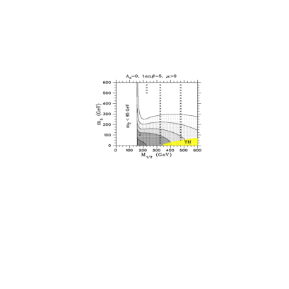
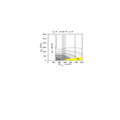
FIG. 1.: The LSP relic density $\Omega_{\tilde{\chi}}\,h_{0}^{2}$ in the ($m_{0}$,$M_{1/2}$) plane for given values of $A_{0}$, $\tan\beta$ and sign of $\mu$. Grey tone regions, from darker to lighter, designate areas in which the LSP relic density takes values in the intervals: $0.00-0.08$, $0.08-0.22$, $0.22-0.35$, $0.35-0.60$ and $0.60-1.00$ respectively. In the blanc area $\Omega_{\tilde{\chi}}\,h_{0}^{2}>1.0$. The area marked by “TH” is theoretically excluded (see main text). The area labelled by $m_{\tilde{C}}<95\;\mathrm{GeV}$ is excluded by chargino searches. Crosses denote points for which thresholds or poles are encountered.

FIG. 2.: The relic density as function of $m_{0}$ for fixed values of the remaining parameters. The solid, dashed and dot-dashed lines correspond to $M_{1/2}=170$, $200$ and $400\;\mathrm{GeV}$ respectively.

FIG. 3.: The relic density as function of $A_{0}$. The lines are as in figure 2.

FIG. 4.: The relic density as function of $\tan\beta$. The lines are as in figure 2.

FIG. 5.: The relic density as function of $M_{1/2}$. Crosses denote points that are near thresholds or poles. The solid (dashed) line corresponds to $m_{0}=150\;(200)\;\mathrm{GeV}$.

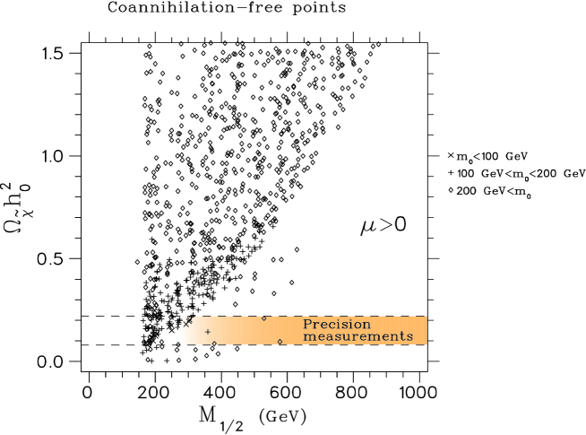
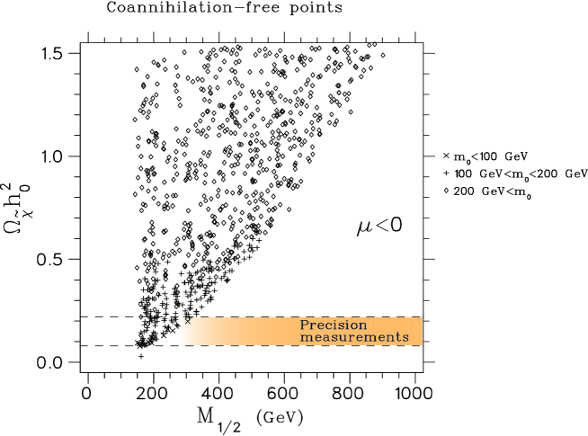
FIG. 6.: Scattered plot of the relic density versus $M_{1/2}$ from a sample of 4000 random points in the parameter space. Low $M_{1/2}$ values are excluded by chargino searches. All points shown are in the coannihilation free region. Only the points with relic density less than 1.5 are shown. The grey tone region within the cosmologically allowed stripe designates the region which agrees with EW precision data (see main text). The horizontal dashed lines mark the limits $0.08<\Omega_{\tilde{\chi}}h_{0}^{2}<0.22$ .

FIG. 7.: Scattered plots of the relic density versus $\tan\beta$ from a sample of random points with fixed $A_{0}=0\;\mathrm{GeV}$, $M_{1/2}=300\;\mathrm{GeV}$. The points shown fall within the coannihilation free region. The two horizontal dashed lines, as in figure 6, mark the cosmologically allowed stripe.

FIG. 8.: The dark-shaded area in figure (a) (figure (b)) designates the cosmologically allowed region $\Omega_{\tilde{\chi}}h_{0}^{2}\;=\;0.15\pm 0.07\;(0.12\pm 0.04)$. The boundary of the coannihilation free region is labelled by $m_{\tilde{\tau}}=1.25\;m_{\tilde{\chi}}$. Also shown is the region in which $m_{\tilde{\tau}}<m_{\tilde{\chi}}$, shaded in light-grey tone. The boundary of the region which is free of color and charged breaking minima, marked as “No CCB”, is also shown. The vertical dashed lines represent the boundaries of the regions $M_{1/2}>200\;\mathrm{GeV}$ and $M_{1/2}>300\;\mathrm{GeV}$.

FIG. 9.: The reduction factor $R(\Delta M)$ as function of $\Delta M=(m_{{\tilde{\tau}}_{R}}-m_{\tilde{\chi}})/m_{\tilde{\chi}}$.

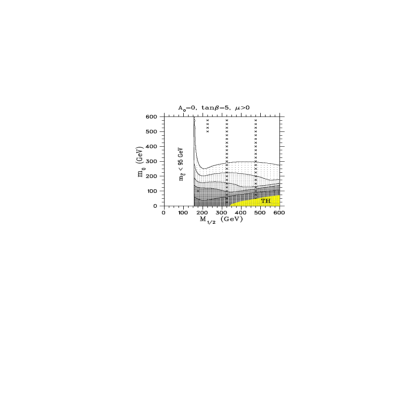
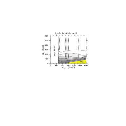
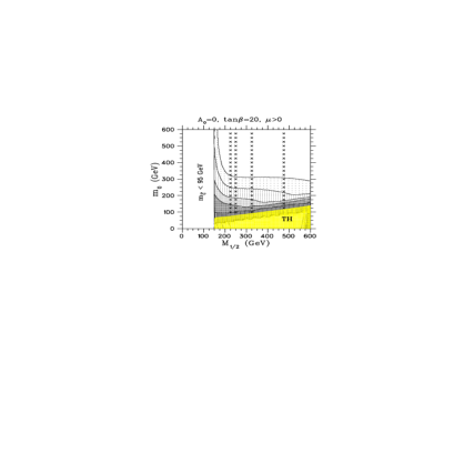
FIG. 10.: The LSP relic density $\Omega_{\tilde{\chi}}\,h_{0}^{2}$ in the ($m_{0}$,$M_{1/2}$) plane for given values of $A_{0}$, $\tan\beta$ and sign of $\mu$ when coannihilation effects are taken into account. The inputs are the same as in figure 1.

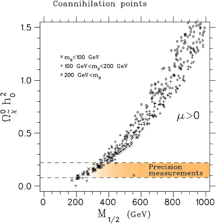
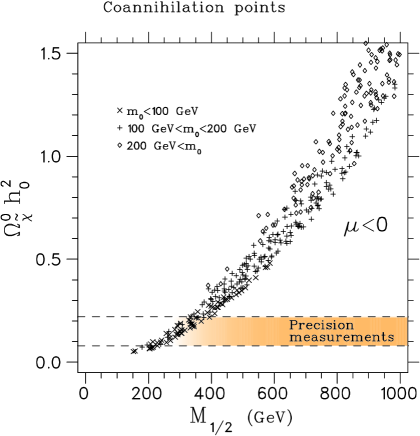
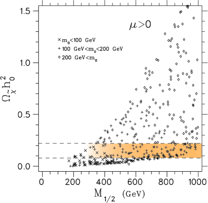
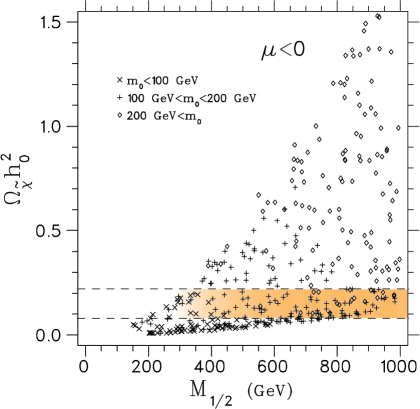
FIG. 11.: The first two figures on the top show the points, from a random sample of 4000 points, which lie entirely within the coannihilation region. The vertical axis refers to $\Omega_{\tilde{\chi}}^{0}\ h_{0}^{2}$ (see main text). The figures at the bottom represent the same situation for the actual relic density $\Omega_{\tilde{\chi}}\ h_{0}^{2}$.

REFERENCES

- [1] “Cosmological parameters”, M. Turner, to be published in the “Particle Physics and Early Universe” (Cosmo ’98), Monterey CA–US, astro-ph/9904051; “Dark matter, dark emergy, and fundamental Physics”, astro-ph/9912211.
- [2] C. Lineweaver, Astrophys. J. Lett. 69 (1998) 505.
- [3] S. Perlmutter et. al., Astrophys. J., in press, astro-ph/9812133.
- [4] A. Riess et. al., Astron. J. 116 (1998) 1009; B. Schmidt et. al., Astrophys. J. 46 (1998) 507.
- [5] B. Chaboyer, Phys. Rep. in press, astro-ph/9808200; W. Freedman, Physica Scripta in press.
- [6] S.D.M. White, J.F. Navarro, A. Evrard and C. Frenk, Nature 366 (1993) 429.
- [7] D. White and A.C. Fabian, MNRAS 273 (1995) 72.
- [8] N.A. Bahcall, J.P. Ostriker, S. Perlmutter and P.J. Steinhardt, Science 284 (1999) 1481.
- [9] J.L. Lopez and D.V. Nanopoulos, Mod. Phys. Lett. A9 (1994) 2755.
- [10] J. Edsjö and P. Gondolo, Phys. Rev. D56 (1997) 1879; P. Gondolo and J. Edsjö, hep-ph/9711461, Talk presented by P. Gondolo at “Topics in Astroparticle and Underground Physics (TAUP) ’97”, Laboratori Nazionali del Gran Sasso – Italy, 7-11 September 1997.
- [11] R. Arnowitt and P. Nath, Mod. Phys. Lett. A13 (1998) 2239.
- [12] J. Wells, Phys. Lett. B443 (1998) 196.
- [13] A.B. Lahanas, D.V. Nanopoulos and V.C. Spanos, Phys. Lett. B464 (1999) 213.
- [14] G.A. Altarelli, R. Barbieri and F. Caravaglios, Int. J. Mod. Phys. A13 (1998) 1031; P. Chankowski and S. Pokorski, “Perspectives in Supersymmetry” edited by G.L. Kane, World Scientific 1997, pp. 402-422, hep-ph/9707497; J. Bagger, K. Matchev, D. Pierce and R. Zhang, Nucl. Phys. B491 (1997) 3; J. Erler and D. Pierce, Nucl. Phys. B526 (1998) 53; A. Dedes, A.B. Lahanas and K. Tamvakis, Phys. Rev. D59 (1999) 015019.
- [15] B. Lee and S. Weinberg, Phys. Rev. Lett. 39 (1977) 165.
- [16] S. Weinberg, Phys. Rev. Lett. 50 (1983) 387; H. Goldberg, Phys. Rev. Lett. 50 (1983) 1419; L.M. Krauss, Nucl. Phys. B227 (1983) 556; J. Ellis, J. Hagelin, D.V. Nanopoulos and M. Srednicki, Phys. Lett. 127B (1983) 233.
- [17] J. Ellis, J. Hagelin, D.V. Nanopoulos, K. Olive and M. Srednicki, Nucl. Phys. B283 (1984) 453; J. Ellis, J. Hagelin and D.V. Nanopoulos, Phys. Lett. 159B (1985) 26; J.S. Hagelin, G.L. Kane and S. Raby, Nucl. Phys. B241 (1984) 638; L.E. Ibañez, Phys. Lett. B137 (1984) 160.
- [18] M. Srednicki, R. Watkins and K.A. Olive, Nucl. Phys. B310 (1988) 693.
- [19] K. Griest, Phys. Rev. D38 (1988) 2357; K. Griest, Phys. Rev. D38 (1988) 2357 [Erratum: D39 (1989) 3802].
- [20] R. Barbieri, M. Friegeni and G.F. Guidice, Nucl. Phys. B313 (1989) 715; J. Ellis, L. Roszkowski and Z. Lalak, Phys. Lett. B245 (1990) 545; J. Ellis, D.V. Nanopoulos, L. Roszkowski and D.N. Schramn, Phys. Lett. B245 (1990) 251; L. Roszkowski Phys. Lett. B252 (1990) 471; Phys. Lett. B262 (1991) 59; J. Ellis and L. Roszkowski, Phys. Lett. B283 (1992) 252; A. Bottino et. al., Astropart. Phys. 1 (1992) 61; R. Roberts and L. Roszkowski, Phys. Lett. B309 (1993) 329; A. Bottino et. al., Astropart. Phys. 2 (1994) 67; G.L. Kane, C. Kolda, L. Roszkowski and J.D. Wells, Phys. Rev. D49 (1994) 6173; E. Diehl, G.L. Kane, C. Kolda and J.D. Wells, Phys. Rev. D52 (1995) 4223.
- [21] K.A. Olive and M. Srednicki, Phys. Lett. B230 (1989) 78; Nucl. Phys. B355 (1991) 208; K. Griest, M. Kamionkowski and M.S. Turner, Phys. Rev. D41 (1990) 3565; J. McDonald, K.A. Olive and M. Srednicki, Phys. Lett. B283 (1992) 80; S. Mizuta, D. Ng and M. Yamaguchi, Phys. Lett. B300 (1993) 96.
- [22] S. Mizuta and M. Yamaguchi, Phys. Lett. B298 (1993) 120.
- [23] J. Ellis and F. Zwirner, Nucl. Phys. B338 (1990) 317; M.M. Nojiri, Phys. Lett. B261 (1991) 76; J.L. Lopez, D.V. Nanopoulos and K. Yuan, Phys. Lett. B267 (1991) 219; J.L. Lopez, D.V. Nanopoulos, H. Pois and K. Yuan, Phys. Lett. B273 (1991) 423; M. Kawasaki and S. Mizuta, Phys. Rev. D46 (1992) 1634; S. Kelley, J.L. Lopez, D.V. Nanopoulos, H. Pois and K. Yuan, Phys. Rev. D47 (1993) 2461.
- [24] J.L. Lopez, D.V. Nanopoulos and K. Yuan, Phys. Rev. D48 (1993) 2766.
- [25] R. Arnowitt and P. Nath, Phys. Lett. B299 (1993) 58 [Erratum: B307 (1993) 403]; Phys. Rev. Lett. 70 (1993) 3696; Phys. Rev. D54 (1996) 2374; M. Drees and A. Yamada, Phys. Rev. D53 (1996) 1586; J. Ellis, T. Falk, K.A. Olive and M. Schmitt, Phys. Lett. B388 (1996) 97.
- [26] J.L. Lopez, D.V. Nanopoulos and K. Yuan, Nucl. Phys. B370 (1992) 445.
- [27] M. Drees and M.M. Nojiri, Phys. Rev. D47 (1993) 376.
- [28] H. Baer and M. Brhlik, Phys. Rev. D53 (1996) 597; V. Barger and C. Kao, Phys. Rev. D57 (1998) 3131.
- [29] For recent review, see G. Jungman, M. Kamionkowski and K. Griest, Phys. Rep. 267 (1996) 195.
- [30] M. Drees, M.M. Nojiri, D.P. Roy and Y. Yamada, Phys. Rev. D56 (1997) 276.
- [31] J. Ellis, T. Falk and K.A. Olive, Phys. Lett. B413 (1998) 355; J. Ellis, T. Falk, K.A. Olive and M. Srednicki, hep-ph/9905481.
- [32] J. Ellis, T. Falk, G. Ganis and K.A. Olive, Phys. Rev. D58 (1998) 095002.
- [33] K. Griest and D. Seckel, Phys. Rev. D43 (1991) 3191.
- [34] P. Gondolo and G. Gelmini, Nucl. Phys. B360 (1991) 145.
- [35] Y. Kawamura, H.P. Nilles, M. Olechowski and M. Yamagushi, JHEP 9806:008 (1998).
- [36] S. Khalil and Q. Shafi, hep-ph/9904448.
- [37] P. Binetruy, G. Giraldi and P. Salati, Nucl. Phys. B237 (1984) 285.
- [38] For review see A.B. Lahanas and D.V. Nanopoulos, Phys. Rep. 145 (1987) 1.
- [39] M.E. Gomez, G. Lazarides and C. Pallis, UT-STPD-7/99, hep-ph/9907261.
- [40] Y. Iwasaki et. al., Z. Phys. C71 (1996) 343; Nucl. Phys. B (Proc. Suppl.) 47 (1996) 515.
- [41] C. Schmid, D.J. Schwarz and P. Widerin, Phys. Rev. D59 (1999) 043517; Phys. Rev. Lett. 78 (1997) 791.
- [42] C. Caso et. al. (Particle Data Group), Euro. Phys. J. C3 (1998) and 1999 partial update for edition 2000 (URL: http://pdg.lbl.gov); LEP2 SUSY working group, LEPSUSYWG/99-01.1 (URL: http://www.cern.ch/LEPSUSY); “Search for charginos and neutralinos in collisions at and mass limit for the lightest neutralino”, EPS-HEP 99, ALEPH 99-011; “Search for charginos and neutralinos production at at LEP”, OPAL coll., CERN-EP/99-123; “Searches for Higgs bosons: Preliminary combined results from the four LEP experiments as ”, ALEPH 99-081 CONF 99-052, DELPHI 99-142 CONF 327, L3 Note 2442, OPAL Technical Note TN-614.
- [43] M. Carena and C. Wagner, hep-ph/9407209; C. Wagner, hep-ph/9510341; W. de Boer et. al., Z. Phys. C71 (1996) 415; M. Carena, P. Chankowski, M. Olechowski, S. Pokorski and C. Wagner, Nucl. Phys. B491 (1997) 103.
- [44] H. Baer, M. Brhlik and D. Castaño, Phys. Rev. D54 (1996) 6944; S. Abel and T. Falk, Phys. Lett. B444 (1998) 427; S. Abel and C. Savoy, Nucl. Phys. B532 (1998) 3.
- [45] H. E. Haber and G. L. Kane, Phys. Rep. 117 (1985) 75; J. F. Gunion and H. E. Haber, Nucl. Phys. B272 (1986) 1.