CERN-TH/99-282
McGill/99-29
hep-ph/9909495

Details on the ${\cal{O}}(m_{e}\alpha^{6})$ Positronium Hyperfine Splitting
due to Single Photon Annihilation

A.H. Hoang^a, P. Labelle^b and S.M. Zebarjad^c

^a Theory Division, CERN,
CH-1211 Geneva 23, Switzerland
^b Department of Physics, McGill University,
Montréal, Québec, Canada H3A 2T8
^c Physics Department and Biruni Observatory,
Shiraz University, Shiraz 71454, Iran

Abstract

A detailed presentation is given of the analytic calculation of the single-photon annihilation contributions for the positronium ground state hyperfine splitting, to order $m_{e}\alpha^{6}$ in the framework of non-relativistic effective theories. The current status of the theoretical description of the positronium ground state hyperfine splitting is reviewed.
PACS numbers: 12.20.Ds, 31.30.Jv, 31.15.Md.

CERN-TH/99-282
September 1999

1 Introduction

Quantum electrodynamics is the prototype of a quantum field theory, and its successes in describing the interactions of leptons and photons have been spectacular. Nevertheless, continuous quantitative tests of QED, particularly at the level of high precision, are important. The positronium system, a two-body bound state consisting of an electron and a positron, provides a clean testing ground of QED because the effects of the strong and the electroweak interactions are negligible, even at the present accuracy of experimental measurements. The existence of positronium was predicted in 1934 [1] based on the relativistic quantum theory developed by Dirac and experimentally verified at the beginning of the 1950s [2]. For the ground state hyperfine splitting, the energy difference between the $1{}^{3}\!S_{1}$ (ortho) and $1{}^{1}\!S_{0}$ (para) states, the most recent experimental values read [3]

$$W\,=\,203\,389.10(74)~{}\mbox{MHz}$$ (1)

and [4, 5]

$$W\,=\,203\,387.5(1.6)~{}\mbox{MHz}\,.$$ (2)

They represent a precision of 3.6 and 7.9 ppm, respectively, which makes the calculation of all ${\cal{O}}(\alpha^{2})$ (NNLO) corrections to the leading and next-to-leading order expression mandatory. Since the dominant contribution to the hyperfine splitting is of order $m_{e}\alpha^{4}$, NNLO corrections correspond to the contributions of order $m_{e}\alpha^{6}$. Including also the known order $m_{e}\alpha^{7}\ln^{2}\alpha^{-1}$ contributions [6, 7] the theoretical expression for the hyperfine splitting reads

$$W\,=\,m_{e}\,\alpha^{4}\,\bigg{[}\,\frac{7}{12}-\frac{\alpha}{\pi}\,\bigg{(}\,\frac{8}{9}+\frac{1}{2}\,\ln 2\,\bigg{)}+\alpha^{2}\,\bigg{(}\,\frac{5}{24}\,\ln\alpha^{-1}+K\,\bigg{)}-\frac{7}{8\pi}\,\alpha^{3}\,\ln^{2}\alpha^{-1}\,\bigg{]}\,,$$ (3)

where $\alpha$ is the fine-structure constant. At order $m_{e}\alpha^{6}$ it is convenient to distinguish between four different sorts of corrections: non-annihilation, single-, two- and three-photon annihilation corrections. The two- and three-photon annihilation contributions have been calculated analytically in Refs. [9] and [10], respectively. The single-photon annihilation contributions have recently been determined in Refs. [11, 12]. In Ref. [12] an analytic result has been presented and in Ref. [11] a numerical one; the two results are in agreement. For the non-annihilation contributions, three different results exist in the literature [13, 14, 15, 16], where Refs. [13, 14, 15] have presented numerical results and Ref. [16] analytical ones. The results of Refs. [14] and [16] are in agreement.

A modern and very economical method to calculate non-relativistic bound state problems is based on the concept of effective field theories. This approach was first proposed in Ref. [13]. The effective field theoretical approach to the positronium bound state problem is based on the existence of widely separated scales in the positronium system. The physical effects associated to these scales are separated by reformulating QED in terms of an effective non-relativistic, non-renormalizable Lagrangian, where the low scale effects correspond to an infinite set of operators and the high scale effects are encoded in the coefficients of the operators. It is the characteristic feature of the effective field theoretical approach that it provides a set of systematic scaling (or power counting) rules that allow for an easy identification of all terms that contribute to a certain order in the bound state calculation. The results presented in Refs. [12, 13, 16] have been obtained within an effective field theory approach. It is the purpose of this paper to present details of the analytical calculation of the order $m_{e}\alpha^{6}$ single-photon annihilation contribution to the hyperfine splitting presented recently in Ref. [12].

The program of this paper is as follows: in Sec. 2 we give an overview of the effective field theory approach to the positronium bound state problem, and we explain the various steps in the calculation of the single-photon annihilation contributions to the hyperfine splitting. Section 3 contains a discussion of the subtleties of the cutoff regularization prescription that we use in our calculation. In Sec. 4 we describe in detail the calculation of the two-loop short-distance coefficient that is needed to determine the single-photon annihilation contributions to the hyperfine splitting at order $m_{e}\alpha^{6}$, and in Sec. 5 we present the bound state calculation, which leads to the final result. A generalization of the result for the single-photon annihilation contributions to the hyperfine splitting to general radial excitations is given in Sec. 6. Section 7 outlines the status of the theoretical calculations of the hyperfine splitting, and Sec. 8 contains a summary. At the end of this work we have attached an appendix where we give a collection of integrals that is useful for the matching calculation.

2 The Conceptual Framework

The dynamics of a non-relativistic $e^{+}e^{-}$ pair bound together in the positronium is governed by three widely separated scales: $m_{e}$, $m_{e}\alpha$ and $m_{e}\alpha^{2}$. Because we are dealing with a Coulombic system, where the electron/positron velocity $v$ is of order $\alpha$ ($v\sim\alpha$), we could equally well talk about the scales $m_{e}v$ and $m_{e}v^{2}$ instead of $m_{e}\alpha$ and $m_{e}\alpha^{2}$. These three scales govern different kinds of physical processes of the positronium dynamics. The hard scale $m_{e}$ is associated with $e^{+}e^{-}$ annihilation and production processes, the dynamics of the small component and photons with virtuality of the order of the electron mass. The soft scale $m_{e}v$ governs the binding of the $e^{+}e^{-}$ pair into a bound state and directly sets the scale of the size of the bound state wave function, the inverse Bohr radius. The ultrasoft scale $m_{e}v^{2}$ is of the order of the binding energy and governs low virtuality photon radiation processes. These processes are associated with higher Fock states, where one has to consider the extended system $e^{+}e^{-}\gamma$ rather than only an electron–positron pair. Because the interactions between the $e^{+}e^{-}$ pair associated with a low virtuality photon can arise with a temporal retardation, the effects caused by these higher Fock states are called “retardation effects”. The Lamb shift in hydrogen is the most famous effect of this sort. The effective field theoretical approach uses the hierarchy of these scales ($m_{e}\gg m_{e}\alpha\gg m_{e}\alpha^{2}$) to successively integrate out momenta of the order of the hard and the soft scale, and, by the same means, to separate the effects associated with them. In this section we give a brief overview onto the conceptual issues involved in this method following Refs. [13, 17, 18, 19]. It is the strength of the effective field theoretical approach that it provides systematical momentum scaling rules (also called power counting rules) which allow an easy identification of all effects that have to be taken into account for a calculation at a specific order. We apply these scaling rules to show that retardation effects do not contribute to the hyperfine splitting at order $m_{e}\alpha^{6}$.

NRQED is the effective field theory, which is obtained from QED after all hard electron/positron and photon momenta, and the respective antiparticle poles associated with the small components have been integrated out. The NRQED Lagrangian reads [13]

$${\cal{L}}_{\mbox{\tiny NRQED}}\,=\,\frac{1}{2}\,(\,{\mbox{\boldmath$E$}}^{2}-{\mbox{\boldmath$B$}}^{2}\,)$$ (4)

$$+\,\psi^{\dagger}\,\bigg{[}\,iD_{t}+c_{2}\,\frac{{\mbox{\boldmath$D$}}^{2}}{2\,m_{e}}+c_{4}\,\frac{{\mbox{\boldmath$D$}}^{4}}{8\,m_{e}^{3}}+\ldots$$

$$\hskip 22.76219pt+\frac{c_{F}\,e}{2\,m_{e}}\,{\mbox{\boldmath$\sigma$}}\cdot{\mbox{\boldmath$B$}}+\,\frac{c_{D}\,e}{8\,m_{e}^{2}}\,(\,{\mbox{\boldmath$D$}}\cdot{\mbox{\boldmath$E$}}-{\mbox{\boldmath$E$}}\cdot{\mbox{\boldmath$D$}}\,)+\frac{c_{S}\,e}{8\,m_{e}^{2}}\,i\,{\mbox{\boldmath$\sigma$}}\,(\,{\mbox{\boldmath$D$}}\times{\mbox{\boldmath$E$}}-{\mbox{\boldmath$E$}}\times{\mbox{\boldmath$D$}}\,)+\ldots\,\bigg{]}\,\psi$$

$$+\,\chi^{\dagger}\,\bigg{[}\,iD_{t}-c_{2}\,\frac{{\mbox{\boldmath$D$}}^{2}}{2\,m_{e}}-c_{4}\,\frac{{\mbox{\boldmath$D$}}^{4}}{8\,m_{e}^{3}}+\ldots$$

$$\hskip 22.76219pt-\frac{c_{F}\,e}{2\,m_{e}}\,{\mbox{\boldmath$\sigma$}}\cdot{\mbox{\boldmath$B$}}+\,\frac{c_{D}\,e}{8\,m_{e}^{2}}\,(\,{\mbox{\boldmath$D$}}\cdot{\mbox{\boldmath$E$}}-{\mbox{\boldmath$E$}}\cdot{\mbox{\boldmath$D$}}\,)+\frac{c_{S}\,e}{8\,m_{e}^{2}}\,i\,{\mbox{\boldmath$\sigma$}}\,(\,{\mbox{\boldmath$D$}}\times{\mbox{\boldmath$E$}}-{\mbox{\boldmath$E$}}\times{\mbox{\boldmath$D$}}\,)+\ldots\,\bigg{]}\,\chi$$

$$-\,\frac{d_{1}\,e^{2}}{4\,m_{e}^{2}}\,(\psi^{\dagger}{\mbox{\boldmath$\sigma$}}\sigma_{2}\chi^{*})\,(\chi^{T}\sigma_{2}{\mbox{\boldmath$\sigma$}}\psi)+\frac{d_{2}\,e^{2}}{3\,m_{e}^{4}}\,\frac{1}{2}\Big{[}\,(\psi^{\dagger}{\mbox{\boldmath$\sigma$}}\sigma_{2}\chi^{*})\,(\chi^{T}\sigma_{2}{\mbox{\boldmath$\sigma$}}(-\mbox{$\frac{i}{2}$}{\stackrel{{\scriptstyle\leftrightarrow}}{{\mbox{\boldmath$D$}}}})^{2}\psi)+\mbox{h.c.}\,\Big{]}+\ldots\,,\,,$$

where $\psi$ and $\chi$ are the electron and positron Pauli spinors; $D_{t}$ and $D$ are the time and space components of the gauge covariant derivative $D_{\mu}$, $E^{i}=F^{0i}$ and $B^{i}=\frac{1}{2}\epsilon^{ijk}F^{jk}$ are the electric and magnetic components of the photon field strength tensor, and $e$ is the electric charge. The short-distance coefficients $c_{2},c_{4},c_{F},c_{D},c_{S},d_{1},d_{2}$, which encode the effects from moments of order $m_{e}$, are normalized to one at the Born level. The subscripts $F$, $D$ and $S$ stand for Fermi, Darwin and spin-orbit. In Eq. (4) only those terms are displayed explicitly that are relevant to the calculation of the single-photon annihilation contributions to the hyperfine splitting at order $m_{e}\alpha^{6}$. The four-fermion operators in the last line of Eq. (4) are of particular importance because their coefficients encode the short-distance (i.e. hard momentum) effects of the single-photon annihilation process. In general, at order $m_{e}\alpha^{6}$ for the ground state hyperfine splitting, the four-fermion operators shown in Eq. (4) would also contain short-distance effects from annihilation into three photons as well as non-annihilation effects, but these are not considered here. The corresponding contributions to the hyperfine splitting have been computed elsewhere, using other techniques (see references given in Secs. 1 and 7). In the following we show explicitly that for the NNLO calculation intended in this work we need the perturbative expansion of the constant $d_{1}$ at order $\alpha^{2}$. For $d_{2}$ the Born contribution is sufficient.

From the above Lagrangian, one may derive explicit Feynman rules, after fixing the gauge. As is well known, the most efficient gauge for non-relativistic calculations is the Coulomb gauge. In that gauge, the Coulomb (or longitudinal) photon (the time component of the vector potential) has an energy (i.e. $k_{0}$) independent propagator, $\langle A_{0}A^{0}\rangle\simeq 1/{\mbox{\boldmath$k$}^{2}}$. This means that the interaction associated with the exchange of a Coulomb photon corresponds to an instantaneous potential. The power counting of diagrams containing instantaneous potentials is particularly simple because an instantaneous propagator has no particle pole, i.e. the scale of $k$ is set by the average momentum of the fermions $\simeq mv$ ($\simeq m\alpha$ in the bound state). On the other hand, the transverse photon (the spatial component of the vector potential) has an energy-dependent propagator, of the form $\langle A_{i}A^{j}\rangle\simeq(\sum\epsilon_{i}\epsilon_{j}^{*})/(k_{0}^{2}-\mbox{\boldmath$k$}^{2})$, where the $\epsilon$ are the physical (transverse) polarization vectors. In that case, the propagator has a particle pole, and $k_{0}$ and $k$ can be of order $mv$ and also of order $mv^{2}$ (with the condition that $k_{0}\leq|\mbox{\boldmath$k$}|$ ([19, 21])). This has the consequence that NRQED diagrams containing transverse photons involve contributions from these two scales and, therefore, do not contribute to a unique order in $v$ (or $\alpha$ in a bound state). This fact can be easily illustrated in the context of old-fashioned (or “time-ordered”) perturbation theory in which the integration over the energy components (via the residues) is done from the very beginning, and one only has to integrate over the spatial momentum components. Usually, the covariant approach is preferred over the old-fashioned perturbation theory because a single covariant diagram contains several time-ordered configurations (which are recovered by performing the contour integration over the energy components). However, the advantage is lost in a non-relativistic application since the different time-ordered diagrams generally scale differently and it is in fact a disadvantage to combine them together. In old-fashioned perturbation theory, one finds that a diagram containing an electron–positron pair and a transverse photon will contain a propagator of the form (see [17] for more details)

$${1\over|\mbox{\boldmath$k$}|}\,{1\over\mbox{\boldmath$p$}_{ext}^{2}/m_{e}-\mbox{\boldmath$p$}^{2}/m_{e}-(\mbox{\boldmath$p$}-\mbox{\boldmath$k$})^{2}/2m_{e}-|\mbox{\boldmath$k$}|}\,,$$ (5)

where $\mbox{\boldmath$p$}_{ext}\simeq\mbox{\boldmath$p$}\simeq m_{e}v$ are the external and loop momenta of the fermions (we are working in the centre-of-mass frame). From this, one can see that different contributions arise depending on whether the scale of $|\mbox{\boldmath$k$}|$ is set by $\mbox{\boldmath$p$}\simeq m_{e}v$ or by $\mbox{\boldmath$p$}^{2}/m_{e}\simeq m_{e}v^{2}$. The effects associated with the latter scale are the retardation effects. The contributions from both momentum regions will not contribute to the same order in $v$. It is, however, possible to generalize NRQED is such a way that the contributions associated to the different scales are coming from separate diagrams. This is achieved by simply Taylor-expanding the NRQED diagrams containing Eq. (5) around $\mbox{\boldmath$k$}\simeq m_{e}v$ and around $\mbox{\boldmath$k$}\simeq m_{e}v^{2}$ (the latter expansion is equivalent to a multipole expansion of the vertices) [17]. One finds that the lowest order term of the expansion around $\mbox{\boldmath$k$}\simeq m_{e}v$ gives a contribution of order

$$\int d^{3}\mbox{\boldmath$k$}\,{1\over|\mbox{\boldmath$k$}|}\,{-1\over|\mbox{\boldmath$k$}|}\simeq{(m_{e}v)^{3}\over(m_{e}v)^{2}}\simeq m_{e}v\,,$$ (6)

whereas the lowest order term of the expansion around $\mbox{\boldmath$k$}\simeq m_{e}v^{2}$ gives

$$\int d^{3}\mbox{\boldmath$k$}\,{1\over|\mbox{\boldmath$k$}|}\,{1\over\mbox{\boldmath$p$}_{ext}^{2}/m_{e}-\mbox{\boldmath$p$}^{2}/m_{e}+k}\simeq{(m_{e}v^{2})^{3}\over(m_{e}v^{2})^{2}}\simeq m_{e}v^{2}.$$ (7)

This shows that the dominant contribution from the transverse photon exchange comes from the scale $\mbox{\boldmath$k$}\simeq m_{e}v$ and that, to leading order, the transverse photon propagator reduces to $-1/\mbox{\boldmath$k$}^{2}$ (which corresponds to simply approximating the transverse photon propagator $1/(k_{0}^{2}-\mbox{\boldmath$k$}^{2})$ by $-1/\mbox{\boldmath$k$}^{2}$). To leading order, the diagrams containing transverse photons are therefore also instantaneous and one recovers the simple power counting rules valid for the exchange of a Coulomb photon. At sub-leading order, things are more complicated, because both expansions must be taken into account but, fortunately, the instantaneous approximation will be sufficient for the present calculation, as will be shown below.

Because the dominant contribution from the exchange of a transverse photon between an electron-positron pair is suppressed by $v^{2}$ compared to the dominant contribution from a Coulomb photon exchange (see the electron/positron–photon couplings involving the $B$ field in Eq. (4)) all interactions at NNLO (i.e. up to order $v^{2}$ with respect to the Coulomb exchange) can be written as a set of simple instantaneous potentials. In momentum space representation they are given by

$$\tilde{V}_{\mbox{\tiny Coul}}({\mbox{\boldmath$p$}},{\mbox{\boldmath$q$}}) = -\,\frac{4\,\pi\,\alpha}{|{\mbox{\boldmath$p$}}-{\mbox{\boldmath$q$}}|^{2}+\lambda^{2}}\,,$$ (8)

$$\tilde{V}_{\mbox{\tiny BF}}({\mbox{\boldmath$p$}},{\mbox{\boldmath$q$}}) = -\,\frac{4\,\pi\,\alpha}{m_{e}^{2}}\,\bigg{[}\,\frac{|{\mbox{\boldmath$p$}\times\mbox{\boldmath$q$}}|^{2}+\frac{\lambda^{2}}{4}|{\mbox{\boldmath$p$}}+{\mbox{\boldmath$q$}}|^{2}}{(|{\mbox{\boldmath$p$}}-{\mbox{\boldmath$q$}}|^{2}+\lambda^{2})^{2}}-\frac{({\mbox{\boldmath$p$}}-{\mbox{\boldmath$q$}})\times{\mbox{\boldmath$S_{-}$}}\cdot({\mbox{\boldmath$p$}}-{\mbox{\boldmath$q$}})\times{\mbox{\boldmath$S_{+}$}}}{|{\mbox{\boldmath$p$}}-{\mbox{\boldmath$q$}}|^{2}+\lambda^{2}}$$ (9)

$$\qquad\quad+\,i\,\frac{3}{2}\,\frac{({\mbox{\boldmath$p$}}\times{\mbox{\boldmath$q$}})\cdot({\mbox{\boldmath$S_{-}$}}+{\mbox{\boldmath$S_{+}$}})}{|{\mbox{\boldmath$p$}}-{\mbox{\boldmath$q$}}|^{2}+\lambda^{2}}-\frac{1}{4}\,\frac{|{\mbox{\boldmath$p$}}-{\mbox{\boldmath$q$}}|^{2}}{|{\mbox{\boldmath$p$}}-{\mbox{\boldmath$q$}}|^{2}+\lambda^{2}}\,\bigg{]}\,,$$

$$\tilde{V}_{4}({\mbox{\boldmath$p$}},{\mbox{\boldmath$q$}}) = \frac{2\,\pi\,\alpha}{m_{e}^{2}}\,d_{1}\,\bigg{[}\,\frac{3}{4}+{\mbox{\boldmath$S_{-}$}}\cdot{\mbox{\boldmath$S_{+}$}}\,\bigg{]}\,,$$ (10)

$$\tilde{V}_{4\mbox{\tiny der}}({\mbox{\boldmath$p$}},{\mbox{\boldmath$q$}}) = -\,\frac{4\,\pi\,\alpha}{3m_{e}^{4}}\,({\mbox{\boldmath$p$}}^{2}+{\mbox{\boldmath$q$}}^{2})\,\bigg{[}\,\frac{3}{4}+{\mbox{\boldmath$S_{-}$}}\cdot{\mbox{\boldmath$S_{+}$}}\,\bigg{]}\,,$$ (11)

$$\delta\tilde{H}_{\mbox{\tiny kin}}({\mbox{\boldmath$p$}},{\mbox{\boldmath$q$}}) = -(2\pi)^{3}\delta^{(3)}(\mbox{\boldmath$p$}-\mbox{\boldmath$q$})\,\ {\mbox{\boldmath$q$}^{4}\over 4m_{e}^{3}}\,.$$ (12)

Here, $\lambda$ is a small fictitious photon mass introduced to regularize infrared divergences, $S_{\mp}$ are the electron/positron spin operators, and $\alpha$ is the fine structure constant; $\tilde{V}_{\mbox{\tiny BF}}$ is the Breit–Fermi potential in the Coulomb gauge, which includes the NNLO relativistic corrections to the Coulomb potential from the longitudinal and transverse photon exchange. The potentials $\tilde{V}_{4}$ and $V_{4\mbox{\tiny der}}$ come from the four-fermion operators in Eq. (4) and account for the single-photon annihilation process at leading order and NNLO in the non-relativistic expansion. For convenience we will also count the NNLO kinetic energy correction in Eq. (12) as a potential.

Using the potentials given above, it is straightforward to derive the momentum space equation of motion for an off-shell, time-independent $e^{+}e^{-}e^{+}e^{-}$ four-point function in the centre-of-mass frame, valid up to NNLO:

$$\bigg{[}\,\frac{\mbox{\boldmath$p$}^{2}}{m_{e}}\,-\,E\,\bigg{]}\,\tilde{G}(\mbox{\boldmath$p$},\mbox{\boldmath$q$};s)\,+\,\int\frac{d^{3}\mbox{\boldmath$q$}^{\prime}}{(2\,\pi)^{3}}\,\tilde{V}(\mbox{\boldmath$p$},\mbox{\boldmath$q$}^{\prime})\,\tilde{G}(\mbox{\boldmath$q$},\mbox{\boldmath$q$}^{\prime};s)\,=\,(2\,\pi)^{3}\,\delta^{(3)}(\mbox{\boldmath$p$}-\mbox{\boldmath$q$})\,,$$ (13)

where

$$E\,\equiv\,\sqrt{s}-2\,m_{e}$$ (14)

is the centre-of-mass energy relative to the electron–positron threshold and

$$\tilde{V}(\mbox{\boldmath$p$},\mbox{\boldmath$q$}) = \tilde{V}_{\mbox{\tiny Coul}}(\mbox{\boldmath$p$},\mbox{\boldmath$q$})+\tilde{V}_{\mbox{\tiny BF}}(\mbox{\boldmath$p$},\mbox{\boldmath$q$})+\tilde{V}_{4}(\mbox{\boldmath$p$},\mbox{\boldmath$q$})+\tilde{V}_{4\,\mbox{\tiny der}}(\mbox{\boldmath$p$},\mbox{\boldmath$q$})+\delta\tilde{H}_{\mbox{\tiny kin}}(\mbox{\boldmath$p$},\mbox{\boldmath$q$})\,.$$ (15)

The equation of motion (13) is a relativistic extension of the non-relativistic Schrödinger equation of the Coulomb problem. Because the potentials $\tilde{V}_{\mbox{\tiny BF}}$, $\tilde{V}_{4}$, $V_{4\mbox{\tiny der}}$ and $\delta\tilde{H}_{\mbox{\tiny kin}}$ lead to ultra-violet divergences, it is important to consider Eq. (13) in the framework of a consistent regularization scheme. The form of the short-distance coefficient $d_{1}$ depends on the choice of the regularization scheme. We will come back to this issue in Sec. 3.

One can easily establish simple power counting rules showing that the potentials given above are all what is needed for our calculation : after factoring out the factors of $1/m_{e}$ that appears explicitly in the potentials, the only scale left in diagrams containing the potentials above is the inverse Bohr radius $\langle\mbox{\boldmath$p$}\rangle\simeq m_{e}\alpha$. In order for the final result to have the dimensions of energy a diagram containing any of the potentials shown above will generate one more factor of $\langle\mbox{\boldmath$p$}\rangle$ than there are factors of inverse electron mass. If there are $n$ factors of $1/m_{e}$, the diagram will therefore generate a factor $\langle\mbox{\boldmath$p$}\rangle^{n+1}/m_{e}^{n}\simeq m_{e}\alpha^{n+1}$. This is one source of powers of $\alpha$. In addition, there are sums over intermediate states. Those contain a factor $1/(E_{ext}-E_{int})$, which scales like $1/(m_{e}\alpha^{2})$. In order to cancel this factor of $1/m_{e}$, the diagram will also generate a factor of $\langle\mbox{\boldmath$p$}\rangle$, which means that each sum over intermediate state brings in another factor of $1/\alpha$. Finally, one must multiply by the explicit factors of $\alpha$ contained in the NRQED vertices and in the short distance coefficients. As a simple illustration of the counting rules, we may consider the Coulomb interaction. The potential contains no inverse power of mass (so $n=0$) and one explicit factor of $\alpha$. In first order of perturbation theory it therefore contributes to order $m_{e}\alpha^{2}$, which is the same order as the contribution coming from the leading order kinetic energy. Adding one more Coulomb potential brings in an extra factor of $\alpha$ from the vertices, but this is cancelled by the inverse power of $\alpha$ generated by the sum over intermediate states. The Coulomb interaction must therefore be summed up to all orders, as is well known. This argument also shows that the Coulomb potential is the only interaction that must be treated exactly, as all the other potentials contain at least two powers of inverse mass so that adding one of those potentials leads to a contribution of order $m\alpha^{4}$ (or higher).

From Eq. (13) we can now derive directly the formula for the single-photon annihilation contribution to the hyperfine splitting at order $m_{e}\alpha^{6}$, $W^{\mbox{\tiny 1-$\gamma$ ann}}_{\mbox{\tiny NNLO}}$. Because the para-positronium state does not contribute, owing to C invariance, one starts with the well-known $n=1$, ${}^{3}S_{1}$ $e^{+}e^{-}$ bound state wave function of the non-relativistic Coulomb problem and determines $W^{\mbox{\tiny 1-$\gamma$ ann}}_{\mbox{\tiny NNLO}}$ via Rayleigh–Schrödinger time-independent perturbation theory. Because we are interested in the single-photon annihilation contributions only corrections with at least one insertion of $\tilde{V}_{4}$ or $\tilde{V}_{4\mbox{\tiny der}}$ have to be taken into account. The formula for $W^{\mbox{\tiny 1-$\gamma$ ann}}$ at order $m_{e}\alpha^{6}$ then reads

$$W^{\mbox{\tiny 1-$\gamma$ ann}} = \langle\,1{}^{3}S_{1}\,|\,V_{4}\,|\,1{}^{3}S_{1}\,\rangle+\langle\,1{}^{3}S_{1}\,|\,V_{4\,\mbox{\tiny der}}\,|\,1{}^{3}S_{1}\,\rangle$$ (16)

$$+\langle\,1{}^{3}S_{1}\,|\,V_{4}\,\sum\int\limits_{l\neq 1{}^{3}S_{1}}\,\frac{|\,l\,\rangle\,\langle\,l\,|}{E_{0}-E_{l}}\,V_{4}\,|\,1{}^{3}S_{1}\,\rangle$$

$$+\,\bigg{[}\,\langle\,1{}^{3}S_{1}\,|\,V_{4}\,\sum\int\limits_{l\neq 1{}^{3}S_{1}}\,\frac{|\,l\,\rangle\,\langle\,l\,|}{E_{0}-E_{l}}\,(V_{\mbox{\tiny BF}}+\delta H_{\mbox{\tiny kin}})\,|\,1{}^{3}S_{1}\,\rangle+\mbox{h.c.}\,\bigg{]}\,+\ldots\,,$$

where $|\,l\,\rangle$ represent normalized (bound state and continuum) eigenstates to the Coulomb Schrödinger equation with the eigenvalues $E_{l}$; $|\,1{}^{3}S_{1}\,\rangle$ and $E_{0}=-m_{e}\alpha^{2}/4$ denote the state and binding energy of the $n=1$, ${}^{3}S_{1}$ Coulomb bound state. Using the counting rules developed above it is easy to show that Eq. (16) is all we need to determine the ground state hyperfine splitting to order $m_{e}\alpha^{6}$: the four-fermion operator $V_{4}$ contains two powers of inverse mass and one explicit factor of $\alpha$ (with the Born level value for the coefficient $d_{1}$, see Eq. (10)). The contribution of this interaction is therefore of order $m_{e}\alpha^{4}$. In order to obtain the ${\cal O}(m_{e}\alpha^{6})$ contribution that we are looking for, we therefore need to match the coefficient $d_{1}$ to two loops, as mentioned above. The operator $V_{\mbox{\tiny 4der}}$, on the other hand, contains four powers of inverse mass and therefore contributes already to order $m_{e}\alpha^{6}$ with the Born level coefficient given in Eq. (11). It is easy to verify that the terms evaluated in second order of perturbation theory also contribute to this order if one uses the Born level coefficients in all the potentials. Consider for example the term with two insertions of the potential $V_{4}$. Since there are four explicit powers of inverse mass, two explicit factors of $\alpha$ (with $d_{1}$ set to 1), and one sum over intermediate states, the final contribution is of order $m_{e}\alpha^{5+2-1}=m_{e}\alpha^{6}$. The Breit potential obviously contributes to the same order. The operator $\delta H_{\mbox{\tiny kin}}$ does not contain any factor of $\alpha$, but it contains one more power of inverse mass and therefore also contributes to order $m_{e}\alpha^{6}$. All other potentials built from the NRQED Feynman rules have higher powers of inverse mass and will therefore be suppressed. We note again that the Breit–Fermi potential $V_{\mbox{\tiny BF}}$ contains contributions arising from the exchange of Coulomb photons and of transverse photons in the instantaneous approximation (i.e. without any $k_{0}$-dependence in the propagator). Since, as we have shown before, the latter contribute already to order $m_{e}\alpha^{6}$, we do not need to consider any sub-leading terms coming from the expansions around $\mbox{\boldmath$k$}\simeq m_{e}v$. Terms from the expansion around $\mbox{\boldmath$k$}\simeq m_{e}v^{2}$ do not need to be considered at all. The instantaneous approximation for the transverse photons is therefore sufficient for the present calculation.

From the above discussion, it is clear that the calculation of $W^{\mbox{\tiny 1-$\gamma$ ann}}_{\mbox{\tiny NNLO}}$ proceeds in two basic steps.

• Matching calculation – Calculation of the ${\cal{O}}(\alpha)$ and ${\cal{O}}(\alpha^{2})$ contributions to the constant $d_{1}$ by matching the QED amplitudes for the elastic s-channel scattering of free and on-shell electrons and positrons via a single photon, $e^{+}e^{-}\to\gamma\to e^{+}e^{-}$, close to threshold up to two loops and to NNLO in the velocity of the electrons and positrons in the centre-of-mass frame. This is possible because the short-distance effects encoded in $d_{1}$ do not depend on the kinematic situation to which the NRQED Lagrangian is applied.

• Bound state calculation – Calculation of formula on the RHS of Eq. (16).

The details of the calculations involved in steps 1 and 2 are presented in Secs. 4 and 5, respectively.

To conclude this section we would also like to briefly mention a formal way to establish the multipole expansion and the counting rules presented above. This is achieved by integrating out NRQED electron/positron and photon momenta of order $m_{e}\alpha$. The resulting effective theory has been called “potential NRQED” (PNRQED) [18]. The basic ingredient to construct PNRQED is to identify the relevant momentum regions of the electron/positron and photon field in the NRQED Lagrangian (4). These momentum regions have been found in Ref. [19]. Because NRQED is not Lorentz-covariant, the time and spatial components of the momenta are independent, which means that the time and spatial components can have a different scaling behaviour. The relevant momentum regions are “soft” ($k^{0}\sim m_{e}v$, $\mbox{\boldmath$k$}\sim m_{e}v$), “potential” ($k^{0}\sim m_{e}v^{2}$, $\mbox{\boldmath$k$}\sim m_{e}v$) and “ultrasoft” ($k^{0}\sim m_{e}v^{2}$, $\mbox{\boldmath$k$}\sim m_{e}v^{2}$). It can be shown that electron, positrons and photons can have soft and potential momenta, but that only photons can have ultrasoft momenta. A momentum region with $k^{0}\sim m_{e}v$, $\mbox{\boldmath$k$}\sim m_{e}v^{2}$ does not exist. PNRQED is constructed by integrating out “soft” electrons/positrons and photons and “potential” photons. In addition, the “potential” photon momenta have to be expanded in terms of their time component, because the latter scales with an additional power of $\alpha$ with respect to the spatial components. The exchange of “potential” photons between the electron and the positron then leads to spatially non-local, but temporally instantaneous, four-fermion operators that represent an instantaneous coupling of an electron–positron pair separated by a distance of order the inverse Bohr radius $\sim m_{e}\alpha$. The coefficients of these operators are a generalization of the notion of an instantaneous potential. Generically the PNRQED Lagrangian has the form

$${\cal{L}}_{\mbox{\tiny PNRQED}} = \tilde{\cal{L}}_{\mbox{\tiny NRQED}}\,+\,\int d^{3}\mbox{\boldmath$r$}\Big{(}\psi^{\dagger}\psi\Big{)}(\mbox{\boldmath$r$})\,V(\mbox{\boldmath$r$})\,\Big{(}\chi^{\dagger}\chi\Big{)}(0)+\ldots\,,$$ (17)

where the tilde above ${\cal{L}}_{\mbox{\tiny NRQED}}$ on the RHS of Eq. (17) indicates that the corresponding operators only describe potential electrons/positrons and ultrasoft photonic degrees of freedom and that an expansion in momentum components $\sim m_{e}\alpha^{2}$ is understood. To NNLO, the contributions to $V$ are just given in Eqs. (8) to (11). Using the scaling of “potential” electron/positron momenta, we see that the Coulomb potential scales like $m_{e}\alpha^{2}$, i.e. it is of the same order as the electron/positron kinetic energy. Thus, the Coulomb potential has to be treated exactly rather than perturbatively. From the PNRQED Lagrangian it is straightforward to derive the momentum space equation of motion of an off-shell, time-independent $(e^{+}e^{-})(e^{+}e^{-})$ four-point function in the centre-of-mass frame valid up to order $\alpha^{4}$, Eq. (13). Using the momentum scaling rules of PNRQED one can show that retardation effects cannot contribute to  $W^{\mbox{\tiny 1-$\gamma$ ann}}$ at order $m_{e}\alpha^{6}$. Retardation effects are caused by the ultrasoft photons, because their low virtuality propagation can develop a pole for the momenta available in the positronium system. Choosing again the Coulomb gauge for our argumentation, where the time component of the Coulomb photon vanishes, only the transverse photon needs to be considered as ultrasoft. Thus the emission and subsequent absorption of an ultrasoft photon between the electron–positron pair are already suppressed by $v^{2}\sim\alpha^{2}$ with respect to the Coulomb interaction owing to the coupling of transverse photon to electrons/positrons. To see that an additional power of $\alpha$ arises from the corresponding loop integration over the ultrasoft photon momentum, let us compare the scaling of the product of the integration measure and the photon propagator in the potential and the ultrasoft momentum regime. In the ultrasoft case the product of the integration measure $d^{4}k$ and the photon propagator $1/k^{2}$ counts as $\alpha^{8}\times\alpha^{-4}=\alpha^{4}$, whereas in the potential case the result reads $\alpha^{5}\times\alpha^{-2}=\alpha^{3}$. Thus the exchange of an ultrasoft photon is suppressed by an addition power of $\alpha$ with respect to the effects of the Breit–Fermi potential (9). In other words, retardation effects cannot contribute to $W^{\mbox{\tiny 1-$\gamma$ ann}}$ at order $m_{e}\alpha^{6}$. We would like to note that PNRQED is designed as a complete field theory capable of describing the dynamics of a bound electron–positron pair and ultrasoft photons. Although useful for establishing consistent counting rules, its full strength only develops if one explicitly considers the dynamics of ultrasoft photons. For cases where the instantaneous approximation is sufficient – such as the ground state hyperfine splitting at order $m_{e}\alpha^{6}$ – the introduction of PNRQED is not essential.

3 The Regularization Scheme

All equations in the previous section have to be considered within the framework of a consistent UV regularization scheme. In general, the form of the short-distance coefficients of the NRQED operators depends on the choice of the regularization scheme. In this work we use a cutoff prescription to regularize the UV divergences, where the cutoff $\Lambda$ is considered much larger than $m_{e}\alpha$. The infrared divergences, which arise in the intermediate steps of the matching calculation to determine the higher order contributions to $d_{1}$, are regularized by a small fictitious photon mass $\lambda$, see Eqs. (8) and (9). The use of a cutoff regularization involves a number of subtleties that shall be briefly discussed in this section.

It is well known that the use of a cutoff regularization scheme leads to terms that violate gauge invariance and Ward identities. These effects, however, are generated at the cutoff and are, therefore, cancelled by corresponding terms with a different sign in the short-distance coefficients of the NRQED operators. Thus, gauge invariance and Ward identities are restored to the order at which the matching calculation has been carried out. Another subtlety is that a cutoff scheme is only well defined after a specific momentum routing convention is adopted for loop diagrams in the effective field theory. It is natural to choose the routing convention employed in the equation of motion (13). For clarity we have illustrated this convention in Fig. 1. Because we only need to consider interactions in our calculation that are instantaneous in time, only ladder-type diagrams have to be taken into account.

                                                    

Figure 1: Routing convention for loop momenta in ladder diagrams. Half of the external centre-of-mass energy is flowing through each of the electron and positron lines.

A very important feature of a cutoff regularization scheme is that it inevitably leads to power-counting-breaking effects. This means that NRQED operators can lead to effects that are below the order indicated by the momentum scaling rules described in the previous section. Examples of this feature will be visible in the matching, and the bound state calculations presented in the next two sections. These power-counting-breaking effects are a consequence of the fact that a cutoff regularization does not suppress divergences of scaleless integrals (as do analytic regularization schemes like $\overline{\mbox{MS}}$). To illustrate the problem let us consider the third term on the RHS of Eq. (16). This term contains the contribution to $W^{\mbox{\tiny 1-$\gamma$ ann}}$ coming from two insertions of the four-fermion operator $V_{4}$. According to the momentum scaling rules described in the previous section, it can only contribute at order $m_{e}\alpha^{6}$. However, the bound state diagram with two $V_{4}$ operators is linearly divergent and, using the momentum cutoff $\Lambda$, the result has, for dimensional reasons, the form $Am_{e}\alpha^{6}+B\Lambda\alpha^{5}$ where $A$ and $B$ are finite constants (modulo logarithmic terms). If one counts the cutoff to be of the order of $m_{e}$, then the diagram would contribute to both orders $m_{e}\alpha^{5}$ and $m_{e}\alpha^{6}$. Even worse, by including sufficiently high order operators (in the $p/m_{e}$ expansion), one can easily convince oneself that an infinite number of operators, having much higher dimension than indicated by the counting rules, would contribute to any given order in $\alpha$, starting at order $m_{e}\alpha^{5}$. However, contributions coming from those higher-dimension operators can only arise in the form of explicit cutoff-dependent terms and not as constants. As for the effects that violate gauge invariance and Ward identities, all terms depending on the cutoff are cancelled in the combination of the bound state integrations and the short-distance coefficient. In our perturbative calculation we can therefore simply ignore that the scaling violating terms coming from operators with dimensions higher than indicated by the counting rules exist. For our calculation this means that we only have to calculate the terms presented on the RHS of Eq. (16), excluding the higher order corrections of $d_{1}$ in the third and fourth terms.

Finally, we would like to mention that we implement our cutoff regularization scheme in such a way that only divergent integrations are actually cut off. This choice simplifies the calculations, because we can use the known analytic solutions of the non-relativistic Coulomb problem for the $1{}^{3}S_{1}$ wave function and the Green function in our perturbative calculation. The fact that we use a specific routing convention ensures that this does not lead to inconsistencies. In addition, we impose the cutoff only on the spatial components of the loop momenta.

4 The Matching Calculation

The single-photon annihilation contributions of the short-distance coefficient of the operator $(\psi^{\dagger}{\mbox{\boldmath$\sigma$}}\sigma_{2}\chi^{*})\,(\chi^{T}\sigma_{2}{\mbox{\boldmath$\sigma$}}\psi)$ are obtained by matching the amplitude for elastic s-channel scattering of an $e^{+}e^{-}$ pair via a virtual photon in full QED in the kinematical regime close to threshold to the same amplitude determined in the non-relativistic effective theory NRQED. To determine the short-distance coefficient $d_{1}$ to order $\alpha^{2}$ we have to carry out the matching at the two-loop level, including all effects up to NNLO in the non-relativistic expansion. Because we regulate infrared divergences in the effective theory using a small fictitious photon mass, we have to do the same in the full QED calculation.

Figure 2: Graphical representation of the NRQED single-photon annihilation scattering diagrams at the Born level and at NNLO in the non-relativistic expansion.

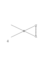
Figure 3: Graphical representation of the NRQED single-photon annihilation scattering diagrams at the one-loop level and at NNLO in the non-relativistic expansion.

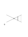
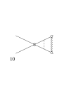
Figure 4: Graphical representation of the NRQED single-photon annihilation scattering diagrams at the two-loop level and at NNLO in the non-relativistic expansion.

   $V_{4}$                         $V_{4\,\mbox{\tiny der}}$                        $\delta H_{\mbox{\tiny kin}}$

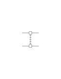
          $V_{\mbox{\tiny Coul}}$                         $V_{\mbox{\tiny BF}}$    

Figure 5: Symbols describing the NRQED potentials that have to be taken into account for the matching calculation at NNLO in the non-relativistic expansion.

To obtain the single-photon scattering amplitude in NRQED we have to calculate the Feynman diagrams depicted in Figs. 2, 3 and 4, where the various symbols are defined in Fig. 5. The Feynman diagrams for the single-photon annihilation contributions of the NRQED scattering amplitude contain, as the formula for $W^{\mbox{\tiny 1-$\gamma$ ann}}$ in Eq. (16), at least one insertion of $V_{4}$ or $V_{4\mbox{\tiny der}}$. As shown in the wave equation (13), we can use time-independent electron–positron propagators also for the NRQED scattering amplitude. This is possible because all interactions are instantaneous in time, i.e. the loop integration over the energy components of the NRQED electron and positron propagators is trivial by residue (see Eq. (26)). Because the single-photon annihilation process is only possible for the electron–positron pair in a ${}^{3}S_{1}$ spin triplet state, we only need to consider the Breit–Fermi potential in the ${}^{3}S_{1}$ configuration:

$$\tilde{V}^{s}_{\mbox{\tiny BF}}(\mbox{\boldmath$p$},\mbox{\boldmath$q$}) = \frac{5}{3}\,\frac{\pi\,\alpha}{m_{e}^{2}}\,\frac{|{\mbox{\boldmath$p$}}-{\mbox{\boldmath$q$}}|^{2}}{|{\mbox{\boldmath$p$}}-{\mbox{\boldmath$q$}}|^{2}+\lambda^{2}}+\frac{\pi\,\alpha}{m_{e}^{2}}\,\frac{(\mbox{\boldmath$p$}^{2}-{\mbox{\boldmath$q$}}^{2})^{2}}{(|\mbox{\boldmath$p$}-\mbox{\boldmath$q$}|^{2}+\lambda^{2})^{2}}-\frac{\pi\,\alpha}{m_{e}^{2}}\,\frac{|\mbox{\boldmath$p$}+\mbox{\boldmath$q$}|^{2}}{|\mbox{\boldmath$p$}-\mbox{\boldmath$q$}|^{2}+\lambda^{2}}\,,$$ (18)

where the angular integration it carried out over the angle between $p$ and $q$. We have eliminated the photon mass in the first term on the RHS of Eq. (18) because it does not lead to any infrared divergences. An additional simplification for the NRQED calculation is obtained by replacing the centre-of-mass energy relative to the $e^{+}e^{-}$ threshold, $E=\sqrt{s}-2m_{e}$, by the new energy parameter $p_{0}$, which is defined as

$$p_{0}^{2}\,\equiv\,\frac{s}{4}-m_{e}^{2}\,.$$ (19)

The parameter $p_{0}$ is equal to the relativistic centre-of-mass three-momentum of the electron/positron in the scattering process. At NNLO in the non-relativistic expansion we have the relation

$$E\,=\,\frac{p_{0}^{2}}{m_{e}}-\frac{p_{0}^{4}}{4\,m_{e}^{3}}+\ldots\,,$$ (20)

where we keep the term $p_{0}^{2}/m_{e}$ in the LO non-relativistic electron–positron propagator. In this convention, the NNLO kinetic energy correction reads

$$\delta H_{\mbox{\tiny kin}}^{*}(\mbox{\boldmath$p$},\mbox{\boldmath$q$})\,=\,-(2\,\pi)^{3}\,\delta^{(3)}(\mbox{\boldmath$p$}-\mbox{\boldmath$q$})\,\frac{\mbox{\boldmath$q$}^{4}-p_{0}^{4}}{4\,m_{e}^{3}}$$ (21)

and simplifies the form of an insertion of the kinetic energy correction

$$\int\frac{d^{3}\mbox{\boldmath$q$}}{(2\pi)^{3}}\,\frac{m_{e}}{\mbox{\boldmath$p$}^{2}-p_{0}^{2}-i\,\epsilon}\,\Big{(}-\delta H_{\mbox{\tiny kin}}^{*}(\mbox{\boldmath$p$},\mbox{\boldmath$q$})\,\Big{)}\,\frac{m_{e}}{\mbox{\boldmath$q$}^{2}-p_{0}^{2}-i\,\epsilon}\,\,=\,\frac{m_{e}}{\mbox{\boldmath$p$}^{2}-p_{0}^{2}-i\,\epsilon}\,\bigg{(}\frac{\mbox{\boldmath$p$}^{2}+p_{0}^{2}}{4\,m_{e}^{3}}\bigg{)}\,.$$ (22)

We emphasize that the introduction of the parameter $p_{0}$ is just a technical trick for the matching calculation, which does not affect the form of $d_{1}$. Using the ${}^{3}S_{1}$ spin average

$$\frac{1}{3}\,\sum_{J=1,0,-1}\Big{[}\,(\psi^{\dagger}{\mbox{\boldmath$\sigma$}}\sigma_{2}\chi^{*})\,(\chi^{T}\sigma_{2}{\mbox{\boldmath$\sigma$}}\psi)\,\Big{]}\,=\,2$$ (23)

for the four-fermion operators $V_{4}$ and $V_{4\mbox{\tiny der}}$ in Eq. (4), we arrive at the following results for the diagrams displayed in Figs. 2, 3 and 4 ($D(\mbox{\boldmath$k$})\equiv m_{e}/(\mbox{\boldmath$k$}^{2}-p_{0}^{2}-i\epsilon)$):

$$I_{1}^{(0)} = \bigg{[}\,1+\Big{(}\frac{\alpha}{\pi}\Big{)}\,d_{1}^{(1)}+\Big{(}\frac{\alpha}{\pi}\Big{)}^{2}\,d_{1}^{(2)}\,\bigg{]}\,\frac{2\,\pi\,\alpha}{m_{e}^{2}}\,,$$ (24)

$$I_{2}^{(0)} = -\,\frac{8\,\pi\,\alpha}{3\,m_{e}^{2}}\,\frac{p_{0}^{2}}{m_{e}^{2}}\,,$$ (25)

$$I_{1}^{(1)} = 2\,i\,\bigg{[}\,1+\Big{(}\frac{\alpha}{\pi}\Big{)}\,d_{1}^{(1)}\,\bigg{]}\,\bigg{(}\frac{2\,\pi\,\alpha}{m_{e}^{2}}\bigg{)}\,\int\frac{d^{4}k}{(2\pi)^{4}}\,\frac{1}{k^{0}+\frac{p_{0}^{2}}{2m_{e}}-\frac{\mbox{\boldmath$k$}^{2}}{2m_{e}}}\,\frac{1}{k^{0}-\frac{p_{0}^{2}}{2m_{e}}+\frac{\mbox{\boldmath$k$}^{2}}{2m_{e}}}\,\frac{4\,\pi\,\alpha}{(\mbox{\boldmath$k$}-\mbox{\boldmath$p_{0}$})^{2}+\lambda^{2}}$$ (26)

$$= 2\,\bigg{[}\,1+\Big{(}\frac{\alpha}{\pi}\Big{)}\,d_{1}^{(1)}\,\bigg{]}\,\bigg{(}\frac{2\,\pi\,\alpha}{m_{e}^{2}}\bigg{)}\,\int\frac{d^{3}\mbox{\boldmath$k$}}{(2\pi)^{3}}\,D(\mbox{\boldmath$k$})\,\frac{4\,\pi\,\alpha}{(\mbox{\boldmath$k$}-\mbox{\boldmath$p_{0}$})^{2}+\lambda^{2}}$$

$$= \bigg{[}\,1+\Big{(}\frac{\alpha}{\pi}\Big{)}\,d_{1}^{(1)}\,\bigg{]}\,\frac{2\,\alpha^{2}}{m_{e}\,p_{0}}\,\bigg{[}\,\frac{\pi^{2}}{2}+i\,\pi\,\ln\Big{(}\frac{2\,p_{0}}{\lambda}\Big{)}\,\bigg{]}\,,$$

$$I_{2}^{(1)} = -2\,\bigg{(}\frac{4\,\pi\,\alpha}{3\,m_{e}^{2}}\bigg{)}\,\int\frac{d^{3}\mbox{\boldmath$k$}}{(2\pi)^{3}}\,\bigg{(}\frac{\mbox{\boldmath$k$}^{2}+p_{0}^{2}}{m_{e}^{2}}\bigg{)}\,D(\mbox{\boldmath$k$})\,\frac{4\,\pi\,\alpha}{(\mbox{\boldmath$k$}-\mbox{\boldmath$p_{0}$})^{2}+\lambda^{2}}$$ (27)

$$= -\,\frac{4\,\alpha^{2}}{3\,m_{e}^{2}}\,\bigg{[}\,\frac{4\,\Lambda}{m_{e}}+\frac{p_{0}\,\pi^{2}}{m_{e}}+2\,i\,\pi\,\frac{p_{0}}{m_{e}}\,\ln\Big{(}\frac{2\,p_{0}}{\lambda}\Big{)}\,\bigg{]}\,,$$

$$I_{3}^{(1)} = 2\,\bigg{(}\frac{2\,\pi\,\alpha}{m_{e}^{2}}\bigg{)}\,\int\frac{d^{3}\mbox{\boldmath$k$}}{(2\pi)^{3}}\,D(\mbox{\boldmath$k$})\,\bigg{(}\frac{\mbox{\boldmath$k$}^{2}+p_{0}^{2}}{4\,m_{e}^{2}}\bigg{)}\,\frac{4\,\pi\,\alpha}{(\mbox{\boldmath$k$}-\mbox{\boldmath$p_{0}$})^{2}+\lambda^{2}}$$ (28)

$$= \frac{\alpha^{2}}{2\,m_{e}^{2}}\,\bigg{[}\,\frac{4\,\Lambda}{m_{e}}+\frac{p_{0}\,\pi^{2}}{m_{e}}+2\,i\,\pi\,\frac{p_{0}}{m_{e}}\,\ln\Big{(}\frac{2\,p_{0}}{\lambda}\Big{)}\,\bigg{]}\,,$$

$$I_{4}^{(1)} = 2\,\bigg{(}\frac{2\,\pi\,\alpha}{m_{e}^{2}}\bigg{)}\,\int\frac{d^{3}\mbox{\boldmath$k$}}{(2\pi)^{3}}\,D(\mbox{\boldmath$k$})\,\Big{(}-\tilde{V}^{s}_{\mbox{\tiny BF}}(\mbox{\boldmath$k$},\mbox{\boldmath$p_{0}$})\,\Big{)}$$ (29)

$$= \frac{\alpha^{2}}{m_{e}^{2}}\,\bigg{[}\,-\frac{10\,\Lambda}{3\,m_{e}}+\frac{p_{0}\,\pi^{2}}{m_{e}}+2\,i\,\pi\,\frac{p_{0}}{m_{e}}\,\bigg{(}\,-\frac{4}{3}+\ln\Big{(}\frac{2\,p_{0}}{\lambda}\Big{)}\,\bigg{)}\,\bigg{]}\,,$$

$$I_{5}^{(1)} = -\,\bigg{(}\frac{2\,\pi\,\alpha}{m_{e}^{2}}\bigg{)}^{2}\,\int\frac{d^{3}\mbox{\boldmath$k$}}{(2\pi)^{3}}\,D(\mbox{\boldmath$k$})\,=\,-\frac{\alpha^{2}}{m_{e}^{2}}\,\bigg{[}\,\frac{2\,\Lambda}{m_{e}}+i\,\pi\,\frac{p_{0}}{m_{e}}\,\bigg{]}\,,$$ (30)

$$I_{1}^{(2)} = \bigg{(}\frac{m_{e}^{2}}{8\,\pi\,\alpha}\bigg{)}\,\Big{[}\,I_{1}^{(1)}\,\Big{]}^{2}\,,$$ (31)

$$I_{2}^{(2)} = 2\,\bigg{(}\frac{2\,\pi\,\alpha}{m_{e}^{2}}\bigg{)}\,\int\frac{d^{3}\mbox{\boldmath$k_{1}$}}{(2\pi)^{3}}\,\int\frac{d^{3}\mbox{\boldmath$k_{2}$}}{(2\pi)^{3}}\,D(\mbox{\boldmath$k_{1}$})\,\frac{4\,\pi\,\alpha}{(\mbox{\boldmath$k_{1}$}-\mbox{\boldmath$k_{2}$})^{2}+\lambda^{2}}\,D(\mbox{\boldmath$k_{2}$})\,\frac{4\,\pi\,\alpha}{(\mbox{\boldmath$k_{2}$}-\mbox{\boldmath$p_{0}$})^{2}+\lambda^{2}}$$ (32)

$$= \frac{\pi\,\alpha^{3}}{2\,p_{0}^{2}}\,\bigg{[}\,\frac{\pi^{2}}{12}-\ln^{2}\Big{(}\frac{2\,p_{0}}{\lambda}\Big{)}+i\,\pi\,\ln\Big{(}\frac{2\,p_{0}}{\lambda}\Big{)}\,\bigg{]}\,,$$

$$I_{3}^{(2)} = -\bigg{(}\frac{4\,\pi\,\alpha}{3\,m_{e}^{2}}\bigg{)}\,\int\frac{d^{3}\mbox{\boldmath$k_{1}$}}{(2\pi)^{3}}\,\int\frac{d^{3}\mbox{\boldmath$k_{2}$}}{(2\pi)^{3}}\,\frac{4\,\pi\,\alpha}{(\mbox{\boldmath$p_{0}$}-\mbox{\boldmath$k_{1}$})^{2}+\lambda^{2}}\,D(\mbox{\boldmath$k_{1}$})\,\bigg{(}\,\frac{\mbox{\boldmath$k_{1}$}^{2}+\mbox{\boldmath$k_{2}$}^{2}}{m_{e}^{2}}\,\bigg{)}\,D(\mbox{\boldmath$k_{2}$})\,\frac{4\,\pi\,\alpha}{(\mbox{\boldmath$k_{2}$}-\mbox{\boldmath$p_{0}$})^{2}+\lambda^{2}}$$ (33)

$$= -\frac{2\,\alpha^{3}}{3\,\pi\,m_{e}\,p_{0}}\,\bigg{[}\,\frac{\pi^{2}}{2}+i\,\pi\,\ln\Big{(}\frac{2\,p_{0}}{\lambda}\Big{)}\,\bigg{]}\,\bigg{[}\,\frac{4\,\Lambda}{m_{e}}+\frac{p_{0}\,\pi^{2}}{2\,m_{e}}+i\,\pi\,\frac{p_{0}}{m_{e}}\,\ln\Big{(}\frac{2\,p_{0}}{\lambda}\Big{)}\,\bigg{]}\,,$$

$$I_{4}^{(2)} = -2\,\bigg{(}\frac{4\,\pi\,\alpha}{3\,m_{e}^{2}}\bigg{)}\,\int\frac{d^{3}\mbox{\boldmath$k_{1}$}}{(2\pi)^{3}}\,\int\frac{d^{3}\mbox{\boldmath$k_{2}$}}{(2\pi)^{3}}\,D(\mbox{\boldmath$k_{1}$})\,\bigg{(}\,\frac{\mbox{\boldmath$p_{0}$}^{2}+\mbox{\boldmath$k_{1}$}^{2}}{m_{e}^{2}}\,\bigg{)}\,\frac{4\,\pi\,\alpha}{(\mbox{\boldmath$k_{1}$}-\mbox{\boldmath$k_{2}$})^{2}+\lambda^{2}}\,D(\mbox{\boldmath$k_{2}$})\,\frac{4\,\pi\,\alpha}{(\mbox{\boldmath$k_{2}$}-\mbox{\boldmath$p_{0}$})^{2}+\lambda^{2}}$$ (34)

$$= -\frac{2\,\alpha^{3}}{3\,m_{e}\,p_{0}}\,\bigg{[}\,\frac{2\,\Lambda}{m_{e}}\,\bigg{(}\pi+2\,i\,\ln\Big{(}\frac{2\,p_{0}}{\lambda}\Big{)}\bigg{)}-\frac{2\,p_{0}\,\pi}{m_{e}}\,\bigg{(}1-\frac{\pi^{2}}{24}+\frac{1}{2}\ln^{2}\Big{(}\frac{2\,p_{0}}{\lambda}\Big{)}-i\,\frac{\pi}{2}\,\ln\Big{(}\frac{2\,p_{0}}{\lambda}\Big{)}\bigg{)}\,\bigg{]}\,,$$

$$I_{5}^{(2)} = \bigg{(}\frac{m_{e}^{2}}{4\,\pi\,\alpha}\bigg{)}\,\Big{[}\,I_{1}^{(1)}\,\Big{]}\,\Big{[}\,I_{3}^{(1)}\,\Big{]}\,,$$ (35)

$$I_{6}^{(2)} = 2\,\bigg{(}\frac{2\,\pi\,\alpha}{m_{e}^{2}}\bigg{)}\,\int\frac{d^{3}\mbox{\boldmath$k_{1}$}}{(2\pi)^{3}}\,\int\frac{d^{3}\mbox{\boldmath$k_{2}$}}{(2\pi)^{3}}\,D(\mbox{\boldmath$k_{1}$})\,\bigg{(}\frac{\mbox{\boldmath$k_{1}$}^{2}+p_{0}^{2}}{4\,m_{e}^{2}}\bigg{)}\,\frac{4\,\pi\,\alpha}{(\mbox{\boldmath$k_{1}$}-\mbox{\boldmath$k_{2}$})^{2}+\lambda^{2}}\,D(\mbox{\boldmath$k_{2}$})\,\frac{4\,\pi\,\alpha}{(\mbox{\boldmath$k_{2}$}-\mbox{\boldmath$p_{0}$})^{2}+\lambda^{2}}$$ (36)

$$= \frac{\alpha^{3}}{4\,m_{e}\,p_{0}}\,\bigg{[}\,\frac{2\,\Lambda}{m_{e}}\,\bigg{(}\pi+2\,i\,\ln\Big{(}\frac{2\,p_{0}}{\lambda}\Big{)}\bigg{)}-\frac{2\,p_{0}\,\pi}{m_{e}}\,\bigg{(}1-\frac{\pi^{2}}{24}+\frac{1}{2}\ln^{2}\Big{(}\frac{2\,p_{0}}{\lambda}\Big{)}-i\,\frac{\pi}{2}\,\ln\Big{(}\frac{2\,p_{0}}{\lambda}\Big{)}\bigg{)}\,\bigg{]}\,,$$

$$I_{7}^{(2)} = 2\,\bigg{(}\frac{2\,\pi\,\alpha}{m_{e}^{2}}\bigg{)}\,\int\frac{d^{3}\mbox{\boldmath$k_{1}$}}{(2\pi)^{3}}\,\int\frac{d^{3}\mbox{\boldmath$k_{2}$}}{(2\pi)^{3}}\,D(\mbox{\boldmath$k_{1}$})\,\frac{4\,\pi\,\alpha}{(\mbox{\boldmath$k_{1}$}-\mbox{\boldmath$k_{2}$})^{2}+\lambda^{2}}\,D(\mbox{\boldmath$k_{2}$})\,\bigg{(}\frac{\mbox{\boldmath$k_{2}$}^{2}+p_{0}^{2}}{4\,m_{e}^{2}}\bigg{)}\,\frac{4\,\pi\,\alpha}{(\mbox{\boldmath$k_{2}$}-\mbox{\boldmath$p_{0}$})^{2}+\lambda^{2}}$$ (37)

$$= \frac{\pi\,\alpha^{3}}{m_{e}^{2}}\,\bigg{[}\,\frac{\pi^{2}}{48}+1-\ln\Big{(}\frac{2\,p_{0}}{\Lambda}\Big{)}-\frac{1}{4}\,\ln^{2}\Big{(}\frac{2\,p_{0}}{\lambda}\Big{)}+i\,\frac{\pi}{2}\,\bigg{(}1+\frac{1}{2}\,\ln\Big{(}\frac{2\,p_{0}}{\lambda}\Big{)}\bigg{)}\,\bigg{]}\,,$$

$$I_{8}^{(2)} = \bigg{(}\frac{m_{e}^{2}}{4\,\pi\,\alpha}\bigg{)}\,\Big{[}\,I_{1}^{(1)}\,\Big{]}\,\Big{[}\,I_{4}^{(1)}\,\Big{]}\,,$$ (38)

$$I_{9}^{(2)} = 2\,\bigg{(}\frac{2\,\pi\,\alpha}{m_{e}^{2}}\bigg{)}\,\int\frac{d^{3}\mbox{\boldmath$k_{1}$}}{(2\pi)^{3}}\,\int\frac{d^{3}\mbox{\boldmath$k_{2}$}}{(2\pi)^{3}}\,D(\mbox{\boldmath$k_{1}$})\,\Big{(}-\tilde{V}^{s}_{\mbox{\tiny BF}}(\mbox{\boldmath$k_{1}$},\mbox{\boldmath$k_{2}$})\,\Big{)}\,D(\mbox{\boldmath$k_{2}$})\,\frac{4\,\pi\,\alpha}{(\mbox{\boldmath$k_{2}$}-\mbox{\boldmath$p_{0}$})^{2}+\lambda^{2}}$$ (39)

$$= \frac{\alpha^{3}}{m_{e}\,p_{0}}\,\bigg{[}\,\frac{\pi\,p_{0}}{m_{e}}\,\bigg{(}\frac{\pi^{2}}{24}+1-\frac{1}{2}\ln 2-2\,\ln\Big{(}\frac{2\,p_{0}}{\Lambda}\Big{)}+\frac{11}{6}\,\ln\Big{(}\frac{2\,p_{0}}{\lambda}\Big{)}-\frac{1}{2}\,\ln^{2}\Big{(}\frac{2\,p_{0}}{\lambda}\Big{)}\bigg{)}$$

$$\hskip 56.9055pt-\frac{5\,\Lambda}{6\,m_{e}}\,\bigg{(}\pi+2\,i\,\ln\Big{(}\frac{2\,p_{0}}{\lambda}\Big{)}\bigg{)}+i\,\frac{\pi^{2}\,p_{0}}{2\,m_{e}}\,\bigg{(}\frac{1}{6}+\ln\Big{(}\frac{2\,p_{0}}{\lambda}\Big{)}\bigg{)}\,\bigg{]}\,,$$

$$I_{10}^{(2)} = 2\,\bigg{(}\frac{2\,\pi\,\alpha}{m_{e}^{2}}\bigg{)}\,\int\frac{d^{3}\mbox{\boldmath$k_{1}$}}{(2\pi)^{3}}\,\int\frac{d^{3}\mbox{\boldmath$k_{2}$}}{(2\pi)^{3}}\,D(\mbox{\boldmath$k_{1}$})\,\frac{4\,\pi\,\alpha}{(\mbox{\boldmath$k_{1}$}-\mbox{\boldmath$k_{2}$})^{2}+\lambda^{2}}\,D(\mbox{\boldmath$k_{2}$})\,$$ (40)

$$\hskip 142.26378pt\times\,\bigg{(}\,2\,\frac{\pi\,\alpha}{m_{e}^{2}}\,\frac{\mbox{\boldmath$k_{2}$}^{2}+p_{0}^{2}}{(\mbox{\boldmath$k_{2}$}-\mbox{\boldmath$p_{0}$})^{2}+\lambda^{2}}-\frac{11}{3}\,\frac{\pi\,\alpha}{m_{e}^{2}}\,\bigg{)}$$

$$= \frac{\pi\,\alpha^{3}}{2\,m_{e}^{2}}\,\bigg{[}\,\frac{\pi^{2}}{12}+4+\ln 2+\frac{10}{3}\,\ln\Big{(}\frac{2\,p_{0}}{\Lambda}\Big{)}-\ln\Big{(}\frac{2\,p_{0}}{\lambda}\Big{)}-\ln^{2}\Big{(}\frac{2\,p_{0}}{\lambda}\Big{)}+i\,\pi\bigg{(}-\frac{7}{6}+\ln\Big{(}\frac{2\,p_{0}}{\lambda}\Big{)}\bigg{)}\,\bigg{]}\,,$$

$$I_{11}^{(2)} = \bigg{(}\frac{m_{e}^{2}}{2\,\pi\,\alpha}\bigg{)}\,\Big{[}\,I_{1}^{(1)}\,\Big{]}\,\Big{[}\,I_{5}^{(1)}\,\Big{]}\,,$$ (41)

$$I_{12}^{(2)} = -\,\bigg{(}\frac{2\,\pi\,\alpha}{m_{e}^{2}}\bigg{)}^{2}\,\int\frac{d^{3}\mbox{\boldmath$k_{1}$}}{(2\pi)^{3}}\,\int\frac{d^{3}\mbox{\boldmath$k_{2}$}}{(2\pi)^{3}}\,D(\mbox{\boldmath$k_{1}$})\,\frac{4\,\pi\,\alpha}{(\mbox{\boldmath$k_{1}$}-\mbox{\boldmath$k_{2}$})^{2}+\lambda^{2}}\,D(\mbox{\boldmath$k_{2}$})\,\,=\,\frac{\pi\,\alpha^{3}}{m_{e}^{2}}\,\bigg{[}\,\ln\Big{(}\frac{2\,p_{0}}{\Lambda}\Big{)}-i\,\frac{\pi}{2}\,\bigg{]}\,.$$ (42)

The upper index of the functions $I_{j}^{(i)}$ corresponds to the power of the fine structure constant of the diagrams and the lower index to the numeration given in Figs. 2, 3 and 4. Combinatorial factors are taken into account. We note that all the above results have been given in the limit $\lambda\ll p_{0}\ll m_{e}$ and that only the powers of $p_{0}$ relevant at NNLO have been kept. A collection of integrals that have been useful in determining the results given above is presented in Appendix. A. The full NRQED amplitude reads

$${\cal{A}}_{\mbox{\tiny NRQED}}^{\mbox{\tiny 1-$\gamma$ ann}} = \sum\limits_{i=1}^{2}\,I^{(0)}_{i}+\sum\limits_{i=1}^{5}\,I^{(1)}_{i}+\sum\limits_{i=1}^{12}\,I^{(2)}_{i}\,.$$ (43)

The elastic single-photon annihilation amplitude in full QED can be obtained from the electromagnetic form factors, which parametrize the radiative corrections to the electromagnetic vertex, and the photon vacuum polarization function. The electromagnetic form factors $F_{1}$ (Dirac) and $F_{2}$ (Pauli) are defined through

$$\bar{u}(p^{\prime})\,\Lambda_{\mu}^{em}\,v(p)\,=\,i\,e\,\bar{u}(p^{\prime})\,\bigg{[}\,\gamma_{\mu}\,F_{1}(q^{2})+\frac{i}{2\,M}\,\sigma_{\mu\nu}\,q^{\nu}\,F_{2}(q^{2})\,\bigg{]}\,v(p)\,,$$ (44)

for the $e^{+}e^{-}$ production vertex, where $q=p+p^{\prime}$ and $\sigma_{\mu\nu}=\frac{i}{2}\,[\,\gamma_{\mu},\gamma_{\nu}\,]$. We need the form factors in the limit $\lambda\ll p_{0}\ll m_{e}$. The one-loop contributions have been known for a long time for all momenta [22, 23], whereas the two-loop contributions have been calculated in the desired limit in Ref. [24]. Parametrizing the loop corrections to the form factors as

$$F_{1}(q^{2}) = 1\,+\,\Big{(}\frac{\alpha}{\pi}\Big{)}\,F_{1}^{(1)}(q^{2})\,+\,\Big{(}\frac{\alpha}{\pi}\Big{)}^{2}\,F_{1}^{(2)}(q^{2})\,+\,\cdots\,,$$

$$F_{2}(q^{2}) = \hskip 22.76228pt\Big{(}\frac{\alpha}{\pi}\Big{)}\,F_{2}^{(1)}(q^{2})\,+\,\Big{(}\frac{\alpha}{\pi}\Big{)}^{2}\,F_{2}^{(2)}(q^{2})\,+\,\cdots\,,$$ (45)

and using the energy parameter $p_{0}$ (Eq. (19)) the results for the form factors in the threshold region at NNLO in the non-relativistic expansion read ($\lambda\ll p_{0}\ll m_{e}$):

$$F_{1}^{(1)}(q^{2}) = i\,\frac{\pi\,m_{e}}{2\,p_{0}}\,\bigg{[}\,\ell-\frac{1}{2}\,\bigg{]}-\frac{3}{2}+i\,\frac{3\,\pi\,p_{0}}{4\,m_{e}}\,\bigg{[}\,\ell-\frac{5}{6}\,\bigg{]}+{\cal{O}}\Big{(}\frac{p_{0}^{2}}{m_{e}^{2}}\Big{)}\,,$$ (46)

$$F_{1}^{(2)}(q^{2}) = \frac{\pi^{2}\,m_{e}^{2}}{8\,p_{0}^{2}}\,\bigg{[}\,-\ell^{2}+\ell-\frac{\pi^{2}}{6}-\frac{1}{3}\,\bigg{]}-i\,\frac{\pi\,m_{e}}{4\,p_{0}}\,\bigg{[}\,3\,\ell-1\,\bigg{]}$$ (47)

$$-\bigg{[}\,\frac{\pi^{4}}{16}+\frac{3\,\pi^{2}}{8}\,\bigg{(}\,\ell^{2}-\frac{4}{3}\,\ell+\frac{46}{45}\,\ln\Big{(}-i\,\frac{p_{0}}{m_{e}}\Big{)}+\frac{7}{15}\,\ln 2+\frac{2729}{1350}\,\bigg{)}$$

$$\hskip 28.45274pt+\frac{9}{80}\,\bigg{(}9\,\zeta_{3}-43\bigg{)}\,\bigg{]}+{\cal{O}}\Big{(}\frac{p_{0}}{m_{e}}\Big{)}\,,$$

$$F_{2}^{(1)}(q^{2}) = i\,\frac{\pi\,m_{e}}{4\,p_{0}}-\frac{1}{2}-i\,\frac{\pi\,p_{0}}{8\,m_{e}}\,+{\cal{O}}\Big{(}\frac{p_{0}^{2}}{m_{e}^{2}}\Big{)}\,,$$ (48)

$$F_{2}^{(2)}(q^{2}) = \frac{\pi^{2}\,m_{e}^{2}}{8\,p_{0}^{2}}\,\bigg{[}\,-\ell+\frac{1}{3}\,\bigg{]}-i\,\frac{\pi\,m_{e}}{4\,p_{0}}\,\bigg{[}\,\ell+1\,\bigg{]}$$ (49)

$$+\bigg{[}\,\frac{\pi^{2}}{8}\,\bigg{(}\,-\ell+\frac{2}{5}\,\ln\Big{(}-i\,\frac{p_{0}}{m_{e}}\Big{)}+\frac{101}{15}\,\ln 2-\frac{1621}{450}\,\bigg{)}$$

$$\hskip 28.45274pt+\frac{1}{80}\,\bigg{(}41\,\zeta_{3}+\frac{347}{9}\bigg{)}\,\bigg{]}+{\cal{O}}\Big{(}\frac{p_{0}}{m_{e}}\Big{)}\,,$$

where

$$\ell\,\equiv\,\ln\Big{(}-\frac{2\,i\,p_{0}}{\lambda}\Big{)}\,.$$ (51)

The photon vacuum polarization function $\Pi$ is defined as

$$(q^{2}\,g^{\mu\nu}-q^{\mu}\,q^{\nu})\,\Pi(q^{2})\,\equiv\,i\,\int d^{4}x\,e^{iqx}\,\langle\,0\,|\,T\,j^{\mu}(x)\,j^{\nu}(0)\,|\,0\,\rangle\,,$$ (52)

where $j^{\nu}$ is the electromagnetic current. The one- and two-loop contributions to $\Pi$ are also known from Refs. [22, 23] for all values of $q^{2}$ and read, expanded up to NNLO in the non-relativistic expansion,

$$\Pi(q^{2}) = \Big{(}\frac{\alpha}{\pi}\Big{)}\,\Pi^{(1)}(q^{2})\,+\,\Big{(}\frac{\alpha}{\pi}\Big{)}^{2}\,\Pi^{(2)}(q^{2})\,+\,\cdots\,,$$ (53)

with

$$\Pi^{(1)}(q^{2}) \stackrel{{\scriptstyle p_{0}\ll m_{e}}}{{=}} \frac{8}{9}+i\,\frac{\pi\,p_{0}}{2\,m_{e}}+{\cal{O}}\Big{(}\frac{p_{0}^{2}}{m_{e}^{2}}\Big{)}\,,$$ (54)

$$\Pi^{(2)}(q^{2}) \stackrel{{\scriptstyle p_{0}\ll m_{e}}}{{=}} -\frac{\pi^{2}}{2}\,\bigg{(}\ln\Big{(}-i\,\frac{p_{0}}{m_{e}}\Big{)}-\frac{11}{16}+\frac{3}{2}\,\ln 2\bigg{)}-\frac{21}{8}\,\zeta_{3}+\frac{3}{4}+{\cal{O}}\Big{(}\frac{p_{0}}{m_{e}}\Big{)}\,.$$ (55)

Including all effects up to NNLO in $p_{0}/m_{e}$ and taking the ${}^{3}S_{1}$ spin average, the QED amplitude reads

$${\cal{A}}_{\mbox{\tiny QED}}^{\mbox{\tiny 1-$\gamma$ ann}} = \bigg{(}\frac{2\,\alpha\,\pi}{m_{e}^{2}}\bigg{)}\,\bigg{(}1-\frac{p_{0}^{2}}{m_{e}^{2}}\bigg{)}\,\frac{1}{1+\Pi(q^{2})}\,\bigg{[}\,\bigg{(}1-\frac{p_{0}^{2}}{6\,m_{e}^{2}}\bigg{)}\,F_{1}(q^{2})+\bigg{(}1+\frac{p_{0}^{2}}{6\,m_{e}^{2}}\bigg{)}\,F_{2}(q^{2})\,\bigg{]}^{2}\,.$$ (56)

The short-distance coefficient $d_{1}$ is determined by requiring equality of all the terms up to order $\alpha^{3}$ and NNLO in $p_{0}/m_{e}$ in the QED and the NRQED amplitudes in Eqs. (56) and (43). The result for $d_{1}$ reads

$$d_{1} = 1+\Big{(}\frac{\alpha}{\pi}\Big{)}\,d_{1}^{(1)}\,+\,\Big{(}\frac{\alpha}{\pi}\Big{)}^{2}\,d_{1}^{(2)}\,+\,\cdots\,,$$ (57)

where

$$d_{1}^{(1)} = \frac{13}{3}\,\frac{\Lambda}{m_{e}}-\frac{44}{9}\,,$$ (58)

$$d_{1}^{(2)} = -\frac{\pi^{2}}{6}\,\ln\Big{(}\frac{\Lambda}{m_{e}}\Big{)}+\frac{13}{8}\,\zeta_{3}-\frac{1483\,\pi^{2}}{288}+\frac{9\,\pi^{2}}{4}\,\ln 2+\frac{1477}{81}\,.$$ (59)

5 The Bound State Calculation

In the final step we have to evaluate the RHS of Eq. (16). It is convenient to perform this calculation also in momentum space representation. In this representation the normalized $n=1$, ${}^{3}S_{1}$ positronium bound state wave function in the non-relativistic limit reads

$$\phi_{0}({\mbox{\boldmath$p$}})\,\equiv\,\langle\mbox{\boldmath$p$}\,|\,1{}^{3}S_{1}\,\rangle\,=\,\frac{8\,\sqrt{\pi}\,\gamma^{5/2}}{({\mbox{\boldmath$p$}}^{2}+\gamma^{2})^{2}}\,,$$ (60)

where

$$\gamma\,\equiv\,\frac{m_{e}\,\alpha}{2}\,.$$ (61)

We also need a momentum space expression for the sum over intermediate Coulomb states in the third and fourth terms on the RHS of Eq. (16). This sum is just the Green function of the non-relativistic Coulomb problem, where the $n=1$, ${}^{3}S_{1}$ ground state pole is subtracted and $E=E_{0}=-m_{e}\alpha^{2}/4$. A compact momentum space integral representation for the Coulomb Green function has been determined by Schwinger [25]:

$$\langle\mbox{\boldmath$p$}\,|\,\sum\int\limits_{l}\,\frac{|\,l\,\rangle\,\langle\,l\,|}{E_{l}-E-i\,\epsilon}\,|\,\mbox{\boldmath$q$}\,\rangle\,=\,\frac{(2\,\pi)^{3}\,\delta^{(3)}(\mbox{\boldmath$p$}-\mbox{\boldmath$q$})\,m_{e}}{\mbox{\boldmath$p$}^{2}-m_{e}\,E-i\,\epsilon}+\frac{m_{e}}{\mbox{\boldmath$p$}^{2}-m\,E-i\,\epsilon}\,\frac{4\,\pi\,\alpha}{(\mbox{\boldmath$p$}-\mbox{\boldmath$q$})^{2}}\,\frac{m_{e}}{\mbox{\boldmath$q$}^{2}-m\,E-i\,\epsilon}$$

$$-\frac{4\,\pi\,\alpha\,m_{e}}{\mbox{\boldmath$p$}^{2}-m\,E-i\,\epsilon}\,\int\limits_{0}^{1}dx\,\frac{i\,\eta\,x^{-i\,\eta}}{(\mbox{\boldmath$p$}-\mbox{\boldmath$q$})^{2}\,x-\frac{1}{4\,m_{e}\,E}\,(\mbox{\boldmath$p$}^{2}-m_{e}\,E-i\,\epsilon)\,(\mbox{\boldmath$q$}^{2}-m_{e}\,E-i\,\epsilon)\,(1-x)^{2}}\,\frac{m_{e}}{\mbox{\boldmath$q$}^{2}}\,,$$

where

$$i\,\eta\,=\,\frac{\alpha}{2}\,\sqrt{\frac{m_{e}}{-E-i\,\epsilon}}\,.$$ (63)

Taking the limit $E\to E_{0}$ the third term on the RHS of Eq. (5) develops the $n=1$, ${}^{3}S_{1}$ pole, $|\phi_{0}({\mbox{\boldmath$p$}})|^{2}/(E_{0}-E)$. After subtraction of this pole, one finds that the momentum space representation of the sum over intermediate states in Eq. (16) can be written as:

$$\langle\mbox{\boldmath$p$}\,|\,\sum\int\limits_{l\neq 1{}^{3}S_{1}}\,\frac{|\,l\,\rangle\,\langle\,l\,|}{E_{0}-E_{l}+i\,\epsilon}\,|\,\mbox{\boldmath$q$}\,\rangle\,=\,-\frac{(2\,\pi)^{3}\,\delta^{(3)}(\mbox{\boldmath$p$}-\mbox{\boldmath$q$})\,m_{e}}{\mbox{\boldmath$p$}^{2}-m_{e}\,E_{0}-i\,\epsilon}$$ (64)

$$-\frac{m_{e}}{\mbox{\boldmath$p$}^{2}-m\,E_{0}-i\,\epsilon}\,\frac{4\,\pi\,\alpha}{(\mbox{\boldmath$p$}-\mbox{\boldmath$q$})^{2}}\,\frac{m_{e}}{\mbox{\boldmath$q$}^{2}-m\,E_{0}-i\,\epsilon}-R(\mbox{\boldmath$p$},\mbox{\boldmath$q$})\,,$$

where

$$R(\mbox{\boldmath$p$},\mbox{\boldmath$q$}) = \frac{64\,\pi\,\gamma^{4}}{\alpha\,(\mbox{\boldmath$p$}^{2}+\gamma^{2})^{2}\,(\mbox{\boldmath$q$}^{2}+\gamma^{2})^{2}}\,\bigg{[}\,\frac{5}{2}-\frac{4\,\gamma^{2}}{\mbox{\boldmath$p$}^{2}+\gamma^{2}}-\frac{4\,\gamma^{2}}{\mbox{\boldmath$q$}^{2}+\gamma^{2}}+\frac{1}{2}\,\ln A$$ (65)

$$\hskip 142.26378pt+\frac{2\,A-1}{\sqrt{4\,A-1}}\arctan\Big{(}\sqrt{4\,A-1}\Big{)}\,\bigg{]}\,,$$

$$A \equiv \frac{(\mbox{\boldmath$p$}^{2}+\gamma^{2})\,(\mbox{\boldmath$q$}^{2}+\gamma^{2})}{4\,\gamma^{2}\,(\mbox{\boldmath$p$}-\mbox{\boldmath$q$})^{2}}\,.$$ (66)

Details of the derivation of expression (65) can be found in Ref. [26]. In Eq.  (64), the three terms correspond to no Coulomb, one Coulomb, and two and more Coulomb potentials in the intermediate state. In the bound state calculation of Eq.(16), the no-Coulomb contributions are linearly divergent, the one-Coulomb contributions are logarithmically divergent and the R-term contributions are finite. In the case of the bound state contributions involving the R terms, the following relation is quite useful ($q\equiv|\mbox{\boldmath$q$}|$) [26]:

$$\int\frac{d^{3}\mbox{\boldmath$p$}}{(2\pi)^{3}}\,R(\mbox{\boldmath$p$},\mbox{\boldmath$q$}) = \frac{8\,\gamma^{3}}{\alpha\,(q^{2}+\gamma^{2})^{2}}\,\bigg{(}\,\frac{5}{2}-\ln 2-\frac{\gamma}{q}\,\arctan\Big{(}\frac{q}{\gamma}\Big{)}+\frac{1}{2}\,\ln\Big{(}1+\frac{q^{2}}{\gamma^{2}}\Big{)}-4\,\frac{\gamma^{2}}{q^{2}+\gamma^{2}}\,\bigg{)}\,.$$ (67)

The results for the individual contributions of the RHS of Eq. (16) read

$$\langle\,1{}^{3}S_{1}\,|\,V_{4}\,|\,1{}^{3}S_{1}\,\rangle\,=\,\int\frac{d^{3}\mbox{\boldmath$k_{1}$}}{(2\pi)^{3}}\,\int\frac{d^{3}\mbox{\boldmath$k_{2}$}}{(2\pi)^{3}}\,\phi_{0}(\mbox{\boldmath$k_{1}$})\,\bigg{[}\frac{2\,\pi\alpha}{m_{e}^{2}}\,d_{1}\bigg{]}\phi_{0}(\mbox{\boldmath$k_{2}$})\,=\,\frac{m_{e}\,\alpha^{4}}{4}\,d_{1}\,,$$ (68)

$$\langle\,1{}^{3}S_{1}\,|\,V_{4\,\mbox{\tiny der}}\,|\,1{}^{3}S_{1}\,\rangle\,=\,\int\frac{d^{3}\mbox{\boldmath$k_{1}$}}{(2\pi)^{3}}\,\int\frac{d^{3}\mbox{\boldmath$k_{2}$}}{(2\pi)^{3}}\,\phi_{0}(\mbox{\boldmath$k_{1}$})\,\bigg{[}-\frac{4\,\pi\alpha}{3\,m_{e}^{2}}\,\frac{\mbox{\boldmath$k_{1}$}^{2}+\mbox{\boldmath$k_{2}$}^{2}}{m_{e}^{2}}\bigg{]}\phi_{0}(\mbox{\boldmath$k_{2}$})$$ (69)

$$= -\frac{2\,m_{e}\,\alpha^{5}}{3\,\pi}\,\frac{\Lambda}{m_{e}}+\frac{m_{e}\,\alpha^{6}}{4}\,,$$

$$\langle\,1{}^{3}S_{1}\,|\,V_{4}\,\sum\int\limits_{l\neq 1{}^{3}S_{1}}\,\frac{|\,l\,\rangle\,\langle\,l\,|}{E_{0}-E_{l}}\,V_{4}\,|\,1{}^{3}S_{1}\,\rangle$$ (70)

$$= \bigg{[}\,-\frac{m_{e}\alpha^{5}}{4\,\pi}\,\frac{\Lambda}{m_{e}}+\frac{m_{e}\alpha^{6}}{16}\,\bigg{]}-\bigg{[}\,\frac{m_{e}\alpha^{6}}{8}\,\ln\Big{(}\frac{\Lambda}{2\,\gamma}\Big{)}\,\bigg{]}-\bigg{[}\,\frac{3\,m_{e}\alpha^{6}}{16}\,\bigg{]}\,,$$

$$\bigg{[}\,\langle\,1{}^{3}S_{1}\,|\,V_{4}\,\sum\int\limits_{l\neq 1{}^{3}S_{1}}\,\frac{|\,l\,\rangle\,\langle\,l\,|}{E_{0}-E_{l}}\,V_{\mbox{\tiny BF}}\,|\,1{}^{3}S_{1}\,\rangle+\mbox{h.c.}\,\bigg{]}\,$$ (71)

$$= -\bigg{[}\,\frac{5\,m_{e}\alpha^{5}}{12\,\pi}\,\frac{\Lambda}{m_{e}}+\frac{m_{e}\alpha^{6}}{4}\,\bigg{(}\frac{1}{12}-\ln\Big{(}\frac{\Lambda}{2\,\gamma}\Big{)}\bigg{)}\,\bigg{]}+\bigg{[}\,\frac{m_{e}\alpha^{6}}{8}\,\bigg{(}-1+\frac{\pi^{2}}{3}-\frac{5}{3}\,\ln\Big{(}\frac{\Lambda}{2\,\gamma}\Big{)}\bigg{)}\,\bigg{]}$$

$$+\bigg{[}\,\frac{m_{e}\alpha^{6}}{4}\,\bigg{(}1-\frac{\pi^{2}}{6}\bigg{)}\,\bigg{]}\,,$$

$$\bigg{[}\,\langle\,1{}^{3}S_{1}\,|\,V_{4}\,\sum\int\limits_{l\neq 1{}^{3}S_{1}}\,\frac{|\,l\,\rangle\,\langle\,l\,|}{E_{0}-E_{l}}\,\delta H_{\mbox{\tiny kin}}\,|\,1{}^{3}S_{1}\,\rangle+\mbox{H.c.}\,\bigg{]}\,$$ (72)

$$= \bigg{[}\,\frac{m_{e}\alpha^{5}}{4\,\pi}\,\frac{\Lambda}{m_{e}}-\frac{15\,m_{e}\alpha^{6}}{128}\,\bigg{]}+\bigg{[}\,\frac{m_{e}\alpha^{6}}{8}\,\bigg{(}-\frac{13}{32}+\ln\Big{(}\frac{\Lambda}{2\,\gamma}\Big{)}\bigg{)}\,\bigg{]}+\bigg{[}\,\frac{51\,m_{e}\alpha^{6}}{256}\,\bigg{]}\,,$$

where, in the last three terms, the results from the no-Coulomb, one-Coulomb and R-terms have been presented in separate brackets. We note that for the bound state calculation we have adopted the usual energy definition as given in Eq. (13). A collection of integrals, which were useful to obtain the results given above, can be found in Ref. [7].

Adding all terms together and taking into account the corrections to $d_{1}$ shown in Eq. (57), we arrive at the final result for the single photon annihilation contributions to the hyperfine splitting at NNLO [12]

$$W^{\mbox{\tiny 1-$\gamma$ ann}} = \frac{m_{e}\alpha^{4}}{4}-\frac{11\,m_{e}\alpha^{5}}{9\,\pi}+\frac{m_{e}\alpha^{6}}{4}\,\bigg{[}\,\frac{1}{\pi^{2}}\,\bigg{(}\,\frac{1477}{81}+\frac{13}{8}\,\zeta_{3}\,\bigg{)}-\frac{1183}{288}+\frac{9}{4}\,\ln 2+\frac{1}{6}\,\ln\alpha^{-1}\,\bigg{]}\,.$$ (73)

The $\ln\alpha^{-1}$ term in Eq. (73) was already known and is included in the $\ln\alpha^{-1}$ contribution quoted in Eq. (3). The single photon annihilation contribution to the constant $K$ defined in Eq. (3) corresponds to a contribution of $-2.34$ MHz to the theoretical prediction of the hyperfine splitting. The same result has been obtained in Ref. [11] using the Bethe–Salpeter formalism and numerical methods.

6 Radial Excitations

From the results presented in the previous sections it would be straightforward to determine the single photon annihilation contributions to the hyperfine splitting for arbitrary radial excitations $n$: we “only” have to redo the bound state calculation shown in the previous section using the general $n{}^{3}S_{1}$ wave functions and the momentum space Coulomb Green function, Eq. (5), where the $n{}^{3}S_{1}$ pole is subtracted. The matching calculation (i.e. the form of the short-distance coefficient $d_{1}$), which does not depend on the non-relativistic dynamics, would remain unchanged. Although such a strategy would be perfectly suited to the general spirit of this work, it would be quite a cumbersome task to work our all the formulae for arbitrary integer values of $n$. (Unlike the contributions to the hyperfine splitting from the annihilation into two [9] and three photons [10], which are pure short-distance corrections and therefore have a trivial dependence on the value of $n$ ($\propto|\phi_{n}(\mbox{\boldmath$0$})|^{2}\sim 1/n^{3}$), the single photon annihilation contributions have a more complicated dependence on the value of $n$ because they involve a non-trivial mixing of bound state and short-distance dynamics.) Thus for the calculation of the single photon annihilation contributions to the hyperfine splitting for arbitrary values of $n$ we use a much simpler method, which one might almost call a “back of the envelope” calculation [12]. However, we emphasize that this method relies more on physical intuition and a careful inspection of the ingredients needed for this specific calculation than on a systematic approach that could be generally used for other problems as well. Nevertheless, this method leads to the correct result, and we therefore present it here as well, following Ref. [12].

We start from the formula for the single photon annihilation contributions to the hyperfine splitting, Eq. (16), generalized to arbitrary values of $n$. (This amounts to replacing “$1{}^{3}S_{1}$” by “$n{}^{3}S_{1}$” everywhere in Eq. (16). In the following we simply refer to this generalized equation as “Eq. (16)”.) Because we use Eq. (16) only to identify two physical quantities from which the single photon contributions to the hyperfine splitting can be derived, we can consider the operators as unrenormalized objects. The relevant physical quantities are easily found if one considers Eq. (16) in configuration space representation, where the operator $V_{4}$ corresponds to a $\delta$-function. From this we see that Eq. (16) depends entirely on the zero-distance Coulomb Green function $A_{n}\equiv\langle\,\mbox{\boldmath$0$}\,|\,\sum_{l\neq n}\int\hskip 14.22636pt\,\frac{|\,l\,\rangle\,\langle\,l\,|}{E_{l}-E_{n}}\,|\,\mbox{\boldmath$0$}\,\rangle$ (where the $n{}^{3}\!S_{1}$ bound state pole is subtracted) and on the rate for the annihilation of an $n{}^{3}\!S_{1}$ bound state into a single photon, $P_{n}\equiv\langle\,n\,|\,V_{4}\,|\,n\,\rangle+[\langle\,n\,|\,V_{4}\,\sum_{l\neq n}\int\hskip 14.22636pt\,\frac{|\,l\,\rangle\,\langle\,l\,|}{E_{n}-E_{l}}\,(V_{\mbox{\tiny BF}}+\delta H_{\mbox{\tiny kin}})\,|\,n\,\rangle+\mbox{h.c.}]+\langle\,n\,|\,V_{4\mbox{\tiny der}}\,|\,n\,\rangle$ (where the effects from $V_{\mbox{\tiny BF}}$ and $\delta H_{\mbox{\tiny kin}}$ are included in the form of corrections to the wave function). Because we have only considered unrenormalized operators, $A_{n}$ and $P_{n}$ are still UV-divergent from the integration over the high energy modes. In the NRQED approach worked out in the previous sections the renormalization was achieved at the level of the operators. Now, the renormalization will be carried out by relating $A_{n}$ and $P_{n}$ to physical (and finite) quantities, which incorporate the proper short-distance physics from the one photon annihilation process. For $A_{n}$ this physical quantity is just the QED vacuum polarization function in the non-relativistic limit and for $P_{n}$ the Abelian contribution of the NNLO expression for the leptonic decay width of a super-heavy quark–antiquark $n{}^{3}\!S_{1}$ bound state [27]. Both quantities have been determined in Refs. [28, 29]. From the results given in Refs. [28, 29] it is straightforward to derive the renormalized versions of $A_{n}$ and $P_{n}$,

$$A^{\mbox{\tiny phys}}_{n} = \frac{m_{e}^{2}}{2\,\pi}\,\bigg{\{}\,\frac{8}{9\,\pi}-\frac{\alpha}{2}\,\bigg{[}\,C_{1}+\bigg{(}\,\ln\Big{(}\frac{\alpha}{2\,n}\Big{)}-\frac{1}{n}+\gamma+\Psi(n)\,\bigg{)}\,\bigg{]}\,\bigg{\}}\,,$$ (74)

$$P^{\mbox{\tiny phys}}_{n} = \frac{2\,\alpha\,\pi}{m_{e}^{2}}\,\bigg{(}\frac{m_{e}^{3}\,\alpha^{3}}{8\,\pi\,n^{3}}\bigg{)}\,\bigg{\{}\,1-4\,\frac{\alpha}{\pi}+\alpha^{2}\,\bigg{[}\,C_{2}-\frac{37}{24\,n^{2}}-\frac{2}{3}\,\bigg{(}\,\ln\Big{(}\frac{\alpha}{2\,n}\Big{)}-\frac{1}{n}+\gamma+\Psi(n)\,\bigg{)}\,\bigg{]}\,\bigg{\}}\,,$$ (75)

where $C_{1}=\frac{1}{2\pi^{2}}(-3+\frac{21}{2}\zeta_{3})-\frac{11}{16}+\frac{3}{2}\ln 2$ and $C_{2}=\frac{1}{\pi^{2}}(\frac{527}{36}-\zeta_{3})+\frac{4}{3}\ln 2-\frac{43}{18}$. Here, $\gamma$ is the Euler constant and $\Psi$ the digamma function. Inserting now $A^{\mbox{\tiny phys}}_{n}$ and $P^{\mbox{\tiny phys}}_{n}$ back into expression (16) we arrive at

$$W^{\mbox{\tiny 1-$\gamma$ ann}}_{n}\,=\,P^{\mbox{\tiny phys}}_{n}\,\bigg{[}\,1-\frac{2\,\alpha\,\pi}{m_{e}^{2}}\,A^{\mbox{\tiny phys}}_{n}+\bigg{(}\,\frac{2\,\alpha\,\pi}{m_{e}^{2}}\,A^{\mbox{\tiny phys}}_{n}\,\bigg{)}^{2}\,\bigg{]}\,.$$ (76)

which leads to [12]

$$W^{\mbox{\tiny 1-$\gamma$ ann}}_{n} = \frac{m_{e}\alpha^{4}}{4\,n^{3}}-\frac{11\,m_{e}\alpha^{5}}{9\,\pi\,n^{3}}$$ (77)

$$+\frac{m_{e}\alpha^{6}}{4\,n^{3}}\,\bigg{\{}\,\frac{1}{2}\,C_{1}+C_{2}+\frac{352}{81\,\pi^{2}}-\frac{37}{24\,n^{2}}+\frac{1}{6}\,\bigg{[}\,\frac{1}{n}+\ln\Big{(}\frac{2\,n}{\alpha}\Big{)}-\gamma-\Psi(n)\,\Bigg{]}\,\bigg{\}}\,.$$

For the ground state $n=1$ Eq. (77) reduces to the result shown in Eq. (73). Equation (77) has also been confirmed by an independent calculation in Ref. [30].

7 Discussion

			Analytical/
	Order	Specification	numerical	Contr. in MHz	Refs.
1	$m_{e}\alpha^{4}$		a	$204\,386.7\mbox{\hskip 19.91692pt}$	[33]
2	$m_{e}\alpha^{5}$		a	$-1\,005.5\mbox{\hskip 19.91692pt}$	[34]
3	$m_{e}\alpha^{6}\ln\alpha^{-1}$		a	$19.1\mbox{\hskip 19.91692pt}$	[8]
4	$m_{e}\alpha^{6}$	non-recoil	a	$-10.43\mbox{\hskip 14.22636pt}$	[35, 30, 16]+[36]
5	$m_{e}\alpha^{6}$	recoil (Caswell–Lepage)	n	$3.1(6)\mbox{\hskip 5.69054pt}$	[13]
6		recoil (Pachucki, Czarnecki et al)	a	$7.02\mbox{\hskip 14.22636pt}$	[14, 16]
7		recoil (Adkins–Sapirstein)	n	$1.32(7)$	[15]
8		1-photon annihilation	a	$-2.34\mbox{\hskip 14.22636pt}$	this work, [11]
9		2-photon annihilation	a	$-0.61\mbox{\hskip 14.22636pt}$	[9]
10		3-photon annihilation	a	$-0.97\mbox{\hskip 14.22636pt}$	[10]
11	$m_{e}\alpha^{7}\ln^{2}\alpha^{-1}$		a	$-0.92\mbox{\hskip 14.22636pt}$	[6, 7]
		Sum (Caswell–Lepage)		$203\,388.1(6)\mbox{\hskip 5.69054pt}$
		Sum (Pachucki, Czarnecki et al)		$203\,392.1\mbox{\hskip 19.91692pt}$
		Sum (Adkins–Sapirstein)		$203\,386.4\mbox{\hskip 19.91692pt}$
		Experiment		$203\,389.1(7)\mbox{\hskip 5.69054pt}$	[3]
				$203\,387.5(1.6)\mbox{}$	[4, 5]

Table 1: Summary of theoretical calculations to the hyperfine splitting and most the most recent experimental measurements.

In Table 1 we have summarized the status of the theoretical calculations to the positronium ground state hyperfine splitting, including our own result. To order $m_{e}\alpha^{6}$ the contribution that it logarithmic in $\alpha$ and the constant one are given separately. The constant terms are further subdivided into non-recoil, recoil, and one-, two- and three-photon annihilation contributions. The non-recoil corrections correspond to diagrams in which one or two photons are emitted and absorbed by the same lepton. (One example is the two-loop contribution to the anomalous magnetic moment.) They are pure short-distance corrections and arise from loop momenta of order $m_{e}$ and above. In the effective field theory approach they are included as a finite renormalization of the coefficients of the NRQED operators. These non-recoil corrections were first evaluated numerically a certain time ago  [35]. More recently, they were calculated analytically by two independent groups  [30, 16] who agreed with each other but disagreed slightly with the numerical result (by about $0.10\,$ MHz). The number we quote in the table is based on the analytical expression. The error of the result at order $m_{e}\alpha^{4}$ in row 1 is of the level of a few $0.01\,$ MHz and not indicated explicitly. It comes from the uncertainties in the Rydberg constant (Ref. [31]) and in $\alpha$ (Ref. [32]). The errors given in rows 5 and 7 are of numerical origin. For all other contributions the errors are negligible. The uncertainties due to the ignorance of the remaining $m_{e}\alpha^{7}\ln\alpha^{-1}$ and $m_{e}\alpha^{7}$ contributions are not taken into account in the summed results.

Except for the recoil corrections, all the quoted results are by now well established. There is still some controversy concerning the recoil corrections for which three different results can be found in the literature. The first calculation was performed by Caswell and Lepage in their seminal paper on NRQED [13]. Recently, new calculations were performed by three different groups, using different techniques. First, Pachucki [14], using an effective field theory approach in coordinate space and a different regularization scheme, obtained a result differing significantly from the one of Caswell and Lepage. Then the Bethe–Salpeter formalism was employed by Adkins and Sapirstein [15], yielding yet another result. Finally, Czarnecki, Melnikov and Yelkhovsky [16] performed the calculation in momentum space with dimensional regularization. They obtained an analytical expression which agrees with Pachucki’s numerical result. The number quoted in the table (row 6) corresponds to their analytical expression.

Comparing with the most recent experimental measurement from Ref. [3], and ignoring remaining theoretical uncertainties, the result containing the Caswell–Lepage calculation for the recoil contributions leads to an agreement between theory and experiment ($W_{\mbox{\tiny th}}-W_{\mbox{\tiny ex}}=-1.0(1.0)$ MHz), whereas the prediction based on the result by Pachucki and Czarnecki et al leads to a discrepancy of more than four standard deviations ($W_{\mbox{\tiny th}}-W_{\mbox{\tiny ex}}=3.0(0.7)$ MHz). On the other hand, the Adkins–Sapirstein result differs by slightly less than four standard deviations but, in contradistinction with Pachucki’s result, it lies below the measured value: ($W_{\mbox{\tiny th}}-W_{\mbox{\tiny ex}}=-2.7(0.7)$ MHz). Recently, the NRQED calculation [13] has been repeated by one of us (P.L.), in collaboration with R. Hill. Preliminary results of this calculation are in contradiction with the original NRQED calculation and also in agreement with Pachucki and Czarnecki et al. Hopefully, the theoretical situation will soon get settled. If the result of Pachucki and Czarnecki et al is indeed confirmed, the significant discrepancy with experiment will have to be addressed.

We note again that we have not included any estimates about the remaining theoretical uncertainties in the considerations given above. The next uncalculated corrections are of order $m_{e}\alpha^{7}\,\ln\alpha^{-1}\approx 0.7$ MHz and could significantly influence the comparison between theory and experiment. However, the coefficient of the log corrections are usually much smaller than 1, and we therefore believe that a contribution of $1$ MHz from the higher order corrections is probably a conservative estimate. In this case, the discrepancy between theory and experiment remains unexplained. Clearly, further work on positronium calculations is necessary.

8 Summary

We have provided the details of the NRQED calculation of the ${\cal O}(m_{e}\alpha^{6})$ contribution to the positronium ground state hyperfine splitting due to single photon annihilation reported in an earlier paper. The counting rules needed to this order have been explained in detail and a discussion on some of the issues related to the use of an explicit cutoff on the momentum integrals has been given. We have provided a list of integrals useful for the evaluation of non-relativistic scattering diagrams. Our result completes the ${\cal O}(m_{e}\alpha^{6})$ calculation of the ground state hyperfine splitting and permits a comparison between theory and experiment at the level of 1 MHz. A comparison with the most recent experimental measurement underlines the need for more theoretical work concerning the ${\cal O}(m_{e}\alpha^{6})$ recoil corrections and higher order contributions.

Appendix A Useful Integrals for the Matching Calculation

In this appendix we present a set of integrals that has been useful for the matching calculations carried out in Sec. 4. All integrals containing ultraviolet divergences are regulated by the cutoff $\Lambda$, where the relation $\Lambda\gg p_{0}$ is implied. Terms of order $1/\Lambda^{k}$, $k>0$ are discarded. As explained in Sec. 2 we have regulated all infrared divergences by using a small fictitious photon mass $\lambda$. In the following we give the results for arbitrary values of $\lambda$, and in an expansion for $\lambda\ll p_{0}$ discarding terms of order $\lambda^{k}$, $k>0$. For the matching calculations presented in this work only the fully expanded results are relevant:

$${\cal{A}}_{1} = \int\limits_{0}^{\Lambda\gg p_{0}}dp\,\frac{p^{2}}{p^{2}-p_{0}^{2}-i\epsilon}\,=\,\Lambda+i\,\pi\,\frac{p_{0}}{2}\,,$$ (78)

$${\cal{A}}_{2} = \int\limits_{0}^{\Lambda\gg p_{0}}dp\,\frac{p^{2}\,(p^{2}-p_{0}^{2})}{(p^{2}+p_{0}^{2}+\lambda^{2})^{2}-4\,p^{2}\,p_{0}^{2}}\,=\,\Lambda-\frac{3}{4}\,\lambda\,\pi\,\stackrel{{\scriptstyle\lambda\to 0}}{{\longrightarrow}}\,\Lambda\,,$$ (79)

$${\cal{A}}_{3} = \int\limits_{0}^{\infty}dp\,\frac{p}{p^{2}-p_{0}^{2}-i\epsilon}\,\ln\bigg{(}\frac{(p+p_{0})^{2}+\lambda^{2}}{(p-p_{0})^{2}+\lambda^{2}}\bigg{)}\,=\,\pi\,\arctan\Big{(}\frac{2\,p_{0}}{\lambda}\Big{)}+i\,\frac{\pi}{2}\,\ln\Big{(}1+\frac{4\,p_{0}^{2}}{\lambda^{2}}\Big{)}$$ (80)

$$\stackrel{{\scriptstyle\lambda\to 0}}{{\longrightarrow}} \frac{\pi^{2}}{2}+i\,\pi\,\ln\Big{(}\frac{2\,p_{0}}{\lambda}\Big{)}\,,$$

$${\cal{A}}_{4} = \int\limits_{0}^{\Lambda\gg p_{0}}dp\,\frac{p^{3}}{p^{2}-p_{0}^{2}-i\epsilon}\,\ln\bigg{(}\frac{(p+p_{0})^{2}+\lambda^{2}}{(p-p_{0})^{2}+\lambda^{2}}\bigg{)}$$ (81)

$$= p_{0}^{2}\,\pi\,\arctan\Big{(}\frac{2\,p_{0}}{\lambda}\Big{)}+p_{0}\,(4\,\Lambda-2\,\pi\,\lambda)+i\,\frac{\pi\,p_{0}^{2}}{2}\,\ln\Big{(}1+\frac{4\,p_{0}^{2}}{\lambda^{2}}\Big{)}$$

$$\stackrel{{\scriptstyle\lambda\to 0}}{{\longrightarrow}} \frac{\pi^{2}}{2}\,p_{0}^{2}+4\,p_{0}\,\Lambda+i\,\pi\,p_{0}^{2}\ln\Big{(}\frac{2\,p_{0}}{\lambda}\Big{)}\,,$$

$${\cal{A}}_{5} = \int\limits_{0}^{\infty}dp\,\frac{p}{(p^{2}+p_{0}^{2}+\lambda^{2})^{2}-4\,p^{2}\,p_{0}^{2}}\,\ln\bigg{(}\frac{(p+p_{0})^{2}+\lambda^{2}}{(p-p_{0})^{2}+\lambda^{2}}\bigg{)}$$ (82)

$$= \frac{\pi}{4\,\lambda\,p_{0}}\,\ln\Big{(}1+\frac{p_{0}^{2}}{\lambda^{2}}\Big{)}\,\stackrel{{\scriptstyle\lambda\to 0}}{{\longrightarrow}}\,\frac{\pi}{2\,\lambda\,p_{0}}\,\ln\Big{(}\frac{p_{0}}{\lambda}\Big{)}\,,$$

$${\cal{A}}_{6} = \int\limits_{0}^{\infty}dp\,\frac{p^{3}}{(p^{2}+p_{0}^{2}+\lambda^{2})^{2}-4\,p^{2}\,p_{0}^{2}}\,\ln\bigg{(}\frac{(p+p_{0})^{2}+\lambda^{2}}{(p-p_{0})^{2}+\lambda^{2}}\bigg{)}$$ (83)

$$= \pi\,\arctan\Big{(}\frac{p_{0}}{\lambda}\Big{)}+\pi\,\frac{p_{0}^{2}-\lambda^{2}}{4\,\lambda\,p_{0}}\,\ln\Big{(}1+\frac{p_{0}^{2}}{\lambda^{2}}\Big{)}\,\stackrel{{\scriptstyle\lambda\to 0}}{{\longrightarrow}}\,\frac{\pi^{2}}{2}+\frac{\pi\,p_{0}}{2\,\lambda}\,\ln\Big{(}\frac{p_{0}}{\lambda}\Big{)}\,,$$

$${\cal{A}}_{7} = \int\limits_{0}^{\infty}dp\,\frac{p}{p^{2}-p_{0}^{2}-i\,\epsilon}\,\frac{1}{(p^{2}+p_{0}^{2}+\lambda^{2})^{2}-4\,p^{2}\,p_{0}^{2}}\,\ln\bigg{(}\frac{(p+p_{0})^{2}+\lambda^{2}}{(p-p_{0})^{2}+\lambda^{2}}\bigg{)}$$ (84)

$$= \frac{\pi}{4\,\lambda^{2}\,p_{0}\,(\lambda^{2}+4\,p_{0}^{2})}\,\bigg{[}\,4\,p_{0}\,\bigg{(}\,\arctan\Big{(}\frac{2\,p_{0}}{\lambda}\Big{)}-\arctan\Big{(}\frac{p_{0}}{\lambda}\Big{)}\,\bigg{)}-\lambda\,\ln\Big{(}1+\frac{p_{0}^{2}}{\lambda^{2}}\Big{)}\,\bigg{]}$$

$$\hskip 56.9055pt+i\,\frac{\pi}{2\,\lambda^{2}\,(\lambda^{2}+4\,p_{0}^{2})}\,\ln\Big{(}1+\frac{4\,p_{0}^{2}}{\lambda^{2}}\Big{)}$$

$$\stackrel{{\scriptstyle\lambda\to 0}}{{\longrightarrow}} \pi\,\bigg{[}\,\frac{4\,p_{0}+i\,\lambda}{32\,\lambda\,p_{0}^{4}}-\frac{1}{8\,\lambda\,p_{0}^{3}}\,\ln\Big{(}\frac{p_{0}}{\lambda}\Big{)}-i\,\frac{\lambda^{2}-4\,p_{0}^{2}}{16\,\lambda^{2}\,p_{0}^{4}}\,\ln\Big{(}\frac{2\,p_{0}}{\lambda}\Big{)}\,\bigg{]}\,,$$

$${\cal{A}}_{8} = \int\limits_{0}^{\infty}dp_{1}\,\int\limits_{0}^{\Lambda\gg p_{0}}dp_{2}\,\frac{p_{1}\,p_{2}}{(p_{1}^{2}-p_{0}^{2}-i\epsilon)\,(p_{2}^{2}-p_{0}^{2}-i\epsilon)}\,\ln\bigg{(}\frac{(p_{1}+p_{2})^{2}+\lambda^{2}}{(p_{1}-p_{2})^{2}+\lambda^{2}}\bigg{)}$$ (85)

$$= \pi^{2}\,\bigg{[}\,\ln\Big{(}\frac{\Lambda}{\lambda}\Big{)}-\frac{1}{2}\,\ln\Big{(}1+\frac{4\,p_{0}^{2}}{\lambda^{2}}\Big{)}+i\,\arctan\Big{(}\frac{2\,p_{0}}{\lambda}\Big{)}\,\bigg{]}$$

$$\stackrel{{\scriptstyle\lambda\to 0}}{{\longrightarrow}} \pi^{2}\,\bigg{[}\,-\ln\Big{(}\frac{2\,p_{0}}{\Lambda}\Big{)}+i\,\frac{\pi}{2}\,\bigg{]}\,,$$

$${\cal{A}}_{9} = \int\limits_{0}^{\infty}dp_{1}\,\int\limits_{0}^{\Lambda\gg p_{0}}dp_{2}\,\frac{p_{1}}{p_{1}^{2}-p_{0}^{2}-i\epsilon}\,\frac{p_{2}\,(p_{2}^{2}-p_{0}^{2})}{(p_{2}^{2}+p_{0}^{2}+\lambda^{2})^{2}-4\,p_{2}^{2}\,p_{0}^{2}}\,\ln\bigg{(}\frac{(p_{1}+p_{2})^{2}+\lambda^{2}}{(p_{1}-p_{2})^{2}+\lambda^{2}}\bigg{)}$$ (86)

$$= -\pi^{2}\,\bigg{[}\,\frac{\lambda}{4\,p_{0}}\,\arctan\Big{(}\frac{p_{0}}{\lambda}\Big{)}+\ln 2+\frac{1}{4}\,\ln\Big{(}1+\frac{p_{0}^{2}}{\lambda^{2}}\Big{)}-\ln\Big{(}\frac{\Lambda}{\lambda}\Big{)}\,\bigg{]}+$$

$$\hskip 56.9055pti\,\pi^{2}\,\bigg{[}\,\frac{1}{2}\,\arctan\Big{(}\frac{p_{0}}{\lambda}\Big{)}-\frac{\lambda}{8\,p_{0}}\,\ln\Big{(}1+\frac{p_{0}^{2}}{\lambda^{2}}\Big{)}\,\bigg{]}$$

$$\stackrel{{\scriptstyle\lambda\to 0}}{{\longrightarrow}} \pi^{2}\,\bigg{(}\,\ln\Big{(}\frac{\Lambda}{\lambda}\Big{)}-\frac{1}{2}\,\ln\Big{(}\frac{p_{0}}{\lambda}\Big{)}-\ln 2\,\bigg{)}+i\,\frac{\pi^{3}}{4}\,,$$

$${\cal{A}}_{10} = \int\limits_{0}^{\infty}dp_{1}\,\int\limits_{0}^{\infty}dp_{2}\,\frac{p_{1}}{(p_{1}^{2}-p_{0}^{2}-i\epsilon)\,(p_{2}^{2}-p_{0}^{2}-i\epsilon)}\,\ln\bigg{(}\frac{(p_{1}+p_{2})^{2}+\lambda^{2}}{(p_{1}-p_{2})^{2}+\lambda^{2}}\bigg{)}\,\ln\bigg{(}\frac{(p_{2}+p_{0})^{2}+\lambda^{2}}{(p_{2}-p_{0})^{2}+\lambda^{2}}\bigg{)}$$ (87)

$$= \frac{\pi^{2}}{p_{0}}\,\bigg{[}\,-\frac{\pi^{2}}{6}+\frac{1}{2}\,\arctan^{2}\Big{(}\frac{2\,p_{0}}{\lambda}\Big{)}-\frac{3}{8}\,\ln^{2}\Big{(}1+\frac{4\,p_{0}^{2}}{\lambda^{2}}\Big{)}-{\rm Li}_{2}\Big{(}-1-\frac{2\,i\,p_{0}}{\lambda}\Big{)}$$

$$\hskip 28.45274pt-{\rm Li}_{2}\Big{(}-1+\frac{2\,i\,p_{0}}{\lambda}\Big{)}\,\bigg{]}$$

$$+i\,\frac{\pi^{2}}{p_{0}}\,\bigg{[}\,\arctan\Big{(}\frac{2\,p_{0}}{\lambda}\Big{)}\,\bigg{(}\ln 2+\ln\Big{(}1+\frac{4\,p_{0}^{2}}{\lambda^{2}}\Big{)}\bigg{)}$$

$$\hskip 14.22636pt+i\,\bigg{(}{\rm Li}_{2}\Big{(}-1+\frac{2\,i\,p_{0}}{\lambda}\Big{)}-{\rm Li}_{2}\Big{(}-1-\frac{2\,i\,p_{0}}{\lambda}\Big{)}+\frac{1}{2}\,{\rm Li}_{2}\Big{(}\frac{1}{2}-\frac{i\,p_{0}}{\lambda}\Big{)}-\frac{1}{2}\,{\rm Li}_{2}\Big{(}\frac{1}{2}+\frac{i\,p_{0}}{\lambda}\Big{)}\bigg{)}\,\bigg{]}$$

$$\stackrel{{\scriptstyle\lambda\to 0}}{{\longrightarrow}} \frac{\pi^{2}}{2\,p_{0}}\,\bigg{[}\,\frac{\pi^{2}}{12}-\ln^{2}\Big{(}\frac{2\,p_{0}}{\lambda}\Big{)}+i\,\pi\ln\Big{(}\frac{2\,p_{0}}{\lambda}\Big{)}\,\bigg{]}\,,$$

$${\cal{A}}_{11} = \int\limits_{0}^{\Lambda\gg p_{0}}dp_{1}\,\int\limits_{0}^{\infty}dp_{2}\,\frac{p_{1}}{p_{2}^{2}-p_{0}^{2}-i\epsilon}\,\ln\bigg{(}\frac{(p_{1}+p_{2})^{2}+\lambda^{2}}{(p_{1}-p_{2})^{2}+\lambda^{2}}\bigg{)}\,\ln\bigg{(}\frac{(p_{2}+p_{0})^{2}+\lambda^{2}}{(p_{2}-p_{0})^{2}+\lambda^{2}}\bigg{)}$$ (88)

$$= 4\,\pi\,\Lambda\,\bigg{[}\,\arctan\Big{(}\frac{2\,p_{0}}{\lambda}\Big{)}+\frac{i}{2}\,\ln\Big{(}1+\frac{4\,p_{0}^{2}}{\lambda^{2}}\Big{)}\,\bigg{]}-2\,\pi^{2}\,p_{0}-2\,\lambda\,\pi^{2}\,\arctan\Big{(}\frac{2\,p_{0}}{\lambda}\Big{)}$$

$$\hskip 28.45274pt-i\,\lambda\,\pi^{2}\,\ln\Big{(}1+\frac{4\,p_{0}^{2}}{\lambda^{2}}\Big{)}$$

$$\stackrel{{\scriptstyle\lambda\to 0}}{{\longrightarrow}} 2\,\Lambda\,\pi^{2}-2\,p_{0}\,\pi^{2}+4\,i\,\Lambda\,\pi\,\ln\Big{(}\frac{2\,p_{0}}{\lambda}\Big{)}\,,$$

$${\cal{A}}_{12} = \int\limits_{0}^{\infty}dp_{1}\,\int\limits_{0}^{\Lambda\gg p_{0}}dp_{2}\,\frac{p_{1}}{p_{1}^{2}-p_{0}^{2}-i\epsilon}\,\ln\bigg{(}\frac{(p_{1}+p_{2})^{2}+\lambda^{2}}{(p_{1}-p_{2})^{2}+\lambda^{2}}\bigg{)}\,\ln\bigg{(}\frac{(p_{2}+p_{0})^{2}+\lambda^{2}}{(p_{2}-p_{0})^{2}+\lambda^{2}}\bigg{)}$$ (89)

$$= \pi^{2}\,\bigg{[}\,-4\,\lambda\,\arctan\Big{(}\frac{p_{0}}{\lambda}\Big{)}+2\,p_{0}\,\bigg{(}\,2-2\,\ln 2-\ln\Big{(}\frac{\lambda^{2}+p_{0}^{2}}{\Lambda^{2}}\Big{)}\,\bigg{)}\,\bigg{]}$$

$$\hskip 14.22636pti\,\pi^{2}\,\bigg{[}\,4\,p_{0}\,\arctan\Big{(}\frac{p_{0}}{\lambda}\Big{)}-2\,\lambda\,\ln\Big{(}1+\frac{p_{0}^{2}}{\lambda^{2}}\Big{)}\,\bigg{]}$$

$$\stackrel{{\scriptstyle\lambda\to 0}}{{\longrightarrow}} 4\,p_{0}\,\pi^{2}\,\bigg{[}\,1-\ln\Big{(}\frac{2\,p_{0}}{\Lambda}\Big{)}+i\,\frac{\pi}{2}\,\bigg{]}\,.$$

References

[1]
S. Mohorovičić,
Astron. Nachr. 253 (1934), 94.
[2]
M. Deutsch, Phys. Rev. 82 (1951) 455;
M. Deutsch and E. Dulit, Phys. Rev. 84 (1951) 601.
[3]
M. W. Ritter, P.O. Egan, V.W. Hughes and K.A. Woodle,
Phys. Rev. A 30 (1984) 1331.
[4]
A. P. Mills, Jr., Phys. Rev. A 27 (1983) 262.
[5]
A. P. Mills, Jr. and G. H. Bearman, Phys. Rev. Lett. 34 (1975) 246.
[8]
G.T. Bodwin and D.R. Yennie, Phys. Reports 43 (1978) 267;
W.E. Caswell and G.P. Lepage, Phys. Rev. A 20 (1979) 36.
[9]
G.S. Adkins, Y.M. Aksu and M.H.T. Bui, Phys. Rev. A 47 (1993) 2640.
[10]
G.S. Adkins, M.H.T. Bui and D. Zhu, Phys. Rev. A 37 (1988) 4071.
[11]
G. S. Adkins, R. N. Fell and P. M. Mitrikov, Phys. Rev. Lett. 79 (1997) 3383.
[12]
A. H. Hoang, P. Labelle and S. M. Zebarjad, Phys. Rev. Lett. 79 (1997) 3387.
[13]
W.E. Caswell and G.E. Lepage, Phys. Lett. B 167 (1986) 437.
[14]
K. Pachucki, Phys. Rev. A 56 (1997) 297.
[15]
G. S. Adkins and J. Sapirstein, Phys. Rev. A 58 (1998) 3552.
[16]
A. Czarnecki, K. Melnikov and A. Yelkhovsky, Phys. Rev. Lett. 82 (1999) 311;
Phys. Rev. A 59 (1999) 4316.
[17]
P. Labelle, Phys. Rev. D 58 (1998) 093013.
[18]
N. Brambilla, A. Pineda, J. Soto and A. Vairo, hep-ph/9903355.
[19]
M. Beneke and V. A. Smirnov, Nucl. Phys. B 522 (1998) 321.
[20]
P. Labelle, S. M. Zebarjad and C. P. Burgess, Phys. Rev. D 56 (1997) 8053.
[21]
H. W. Griesshammer, Phys. Rev. D 58 (1998) 094027.
[22]
G. Källen and A. Sabry,
K. Dan. Vidensk. Selsk. Mat.-Fys. Medd.29 (1955) No. 17.
[23]
J. Schwinger, Particles, Sources and Fields,
Vol II (Addison-Wesley, New York, 1973).
[24]
A. H. Hoang, Phys. Rev. D 56 (1997) 7276.
[25]
J. Schwinger, J. Math. Phys. 5 (1964) 1606.
[26]
W. E. Caswell and G. P. Lepage, Phys. Rev. A 18 (1978) 810.
[27]
G.T. Bodwin, E. Braaten and G.P. Lepage, Phys. Rev. D 51 (1995) 1125.
[28]
A.H. Hoang, Phys. Rev. D 57 (1998) 1615.
[29]
A.H. Hoang, Phys. Rev. D 56 (1997) 5851.
[30]
K. Pachucki and S. G. Karshenboǐm, Phys. Rev. Lett. 80 (1998) 2101.
[31]
T. Udem, et al.,
Phys. Rev. Lett. 79 (1997) 2646.
[32]
Particle Data Group,
C. Caso et al., Eur. Phys. J. C 3 (1998) 1.
[33]
J. Pirenne,
Arch. Sci. Phys. Nat. 28 (1946) 233.
[34]
R. Karplus and A. Klein, Phys. Rev. 87 (1952) 848.
[35]
J.R. Sapirstein, E.A. Terray and D.R. Yennie, Phys. Rev. D 29 (1984) 2290.
[36]
A trivial correction to order is obtained by including
the anomalous magnetic moment to two loops in the lowest order
Fermi correction, which leads to an contribution
equal to
MHz.
We are grateful to G. Adkins for bringing to our attention that this
correction was not included in some of the earlier references.