${\rm Bari-TH/99-361}$ ${\rm Napoli-DSF~{}99/32}$
$B\to\pi\pi\ell\nu_{\ell}$ decays
in a QCD relativistic potential model

In the framework of a QCD relativistic potential model we evaluate the form factors describing the exclusive decay $B\to\pi\pi\ell\nu$. The calculation is performed in a phase space region far away from the resonances and therefore is complementary to other decay mechanisms where the pions are produced by intermediate particles, e.g. in the chiral approach. We give an estimate of the contribution of the non resonant channel of the order of $\mathcal{B}$$(B^{-}\to\pi^{+}\pi^{-}\ell^{-}\bar{\nu}_{\ell})\simeq 2.2\times 10^{-4}$.

In this letter we shall study the $B-$meson decays

$$B^{-}\to\pi^{+}\pi^{-}\ell^{-}\bar{\nu}_{\ell}$$ (1)

$$\bar{B}^{0}\to\pi^{+}\pi^{0}\ell^{-}\bar{\nu}_{\ell}~{}.$$ (2)

¿From the experimental side these decays are interesting in view of the future programs at the $B$-factories. For example, some of the preliminary studies on the CP violations at these machines [1] have examined the possibility to extract the angle $\alpha$ of the unitarity triangle by the $B\to\rho\pi$ non leptonic decay channel. The non-resonant decay mode $B\to\ 3\pi$ would be interesting to analyze in this context, as it might provide a significant background to the main decay process. While a calculation from first principles is not available at the moment, a useful approximation might be the factorization approximation and, within this approximation, the decay modes (1) and (2) would provide the crucial hadronic matrix elements needed to compute the relevant amplitudes. In passing we note that there is another channel, i.e. the $B^{-}\to\pi^{0}\pi^{0}\ell^{-}\bar{\nu}_{\ell}$ decay mode, which will not be examined here because it is less interesting from an experimental point of view.

¿From a theoretical standpoint semileptonic $B$-meson decays with two hadrons in the final state represent a formidable challenge as they involve hadronic matrix elements of weak currents with three hadrons. They can be studied by pole diagrams, which amounts to a simplification because only two hadrons are involved in the hadronic matrix elements. This is the approach followed in some papers where these decays have been examined in the framework of the chiral perturbation theories for heavy meson decays [2],[3]. This method is based on an effective theory implementing both heavy-quark and chiral symmetry [3], [4], [5], [6] and allows to achieve, for systems comprising both heavy ($Q$) and light ($q$) quarks, rigorous results in the combined $m_{Q}\to\infty,~{}m_{q}\to 0$ limit. However the range of validity of this approach is limited by the requirement of soft pion momenta. In the soft pion limit the amplitude is dominated by a few tree diagrams with resonances as intermediate states, and some clear predictions can be made, but, at least for $B$ decays, the actual phase space is relatively large and the phenomenological interest of these predictions is modest. The aim of this letter is to examine the decays (1) and (2) in the framework of a QCD relativistic potential model [7] and to extend the kinematical range where theoretical predictions are possible. We shall present a detailed analysis of the four form factors relevant to (1); for reasons of space we shall only give a prediction for the width of the decay (2). We shall not include final state interactions in our calculation since no consistent way to compute them is presently available. It’s clear however that they can modify our numerical calculations [8].

In two recent papers: [9] ,[10] we have presented an analysis of some semileptonic and rare $B$ decays into one light hadron employing the relativistic potential model in an approximation that renders the calculations simpler. We wish to exploit here this approximation in the study of the $B\to\pi\pi\ell\nu$ decays .

Let us start with a description of the model (for more details see [7], [9] and [10]). In this approach the mesons are described as bound states of constituent quarks and antiquarks tied by an instantaneous potential $V(r)$, which has a confining linear behaviour at large interquark distances $r$ and a Coulombic behaviour $\simeq-\alpha_{s}(r)/r$ at small distances, with $\alpha_{s}(r)$ the running strong coupling constant (the Richardson’s potential [11] is used to interpolate between the two regions). Due to the nature of the interquark forces, the light quarks are relativistic; for this reason one employs for the meson wave function $\Psi$ the Salpeter [12] equation embodying the relativistic kinematics:

$$\left[\sqrt{-\nabla_{1}^{2}+m^{2}_{1}}+\sqrt{-\nabla_{2}^{2}+m^{2}_{2}}+V(r)\right]\Psi(\vec{r})=M\Psi(\vec{r})~{}\;\;,$$ (3)

where the index 1 refers to the heavy quark and the index 2 to the light antiquark; $M$ is the heavy meson mass that is obtained by fitting the various parameters of the model, in particular the b-quark mass, that is fitted to the value $m_{b}=4890$ MeV, and the light quark masses $m_{u}\simeq m_{d}=38$ MeV, $m_{s}=115$ MeV. The $B$-meson wave function $\Psi(\vec{r})$ in its rest frame is obtained by solving eq. (3); a useful representation in Fourier momentum space was obtained in [9] and is as follows

$$\psi(k)=4\pi\sqrt{m_{B}\alpha^{3}}\ e^{-\alpha k}\;\;,$$ (4)

with $\alpha=2.4$ GeV^-1 and $k=|\vec{k}|$ the quark momentum in the $B$ rest frame; this is the first approximation introduced in [9].

The constituent quark picture used in the model is rather crude. There are no propagating gluons in the instantaneous approximation : the Coulombic interaction is assumed to be static. Moreover, the complex structure of the hadronic vacuum is simplified: the confinement can be introduced by the linearly rising potential at large distances, but the chiral symmetry and the Nambu-Goldstone boson nature of the $\pi$’s cannot be implemented by the constituent quark picture. For these reasons, while there are good reasons to believe that eq. (3) may describe the quark distribution inside the heavy meson, one cannot pretend to apply it to light mesons. Therefore pion couplings to the quark degrees of freedom are described by effective vertices.

To evaluate the amplitude for semileptonic decays, it is useful to follow some simple rules, similar to the Feynman rules by which the amplitudes are computed in perturbative field theory. The setting of these rules is the main innovation introduced in [9] as compared to [7]. For the decays (1) and (2) we draw a quark-meson diagram as in fig. 1 and we evaluate it according to the following rules:

1) for a charged pion of momentum $p_{\pi}$ we write the coupling

$$-\frac{N_{q}\ N_{q^{\prime}}}{f_{\pi}}\not\!p_{\pi}\,\gamma_{5}\;\;,$$ (5)

where $f_{\pi}=130\ MeV$. The normalization factors $N_{q},~{}N_{q^{\prime}}$ for the quark coupled to the meson are discussed below;
2) for the heavy meson $B$ in the initial state one introduces the matrix:

$$B=\frac{1}{\sqrt{3}}\psi(k){\sqrt{\frac{m_{q}m_{b}}{m_{q}m_{b}+q_{1}\cdot q_{2}}}}\;\;\frac{\not\!q_{1}\,+m_{b}}{2m_{b}}(-i\ \gamma_{5})\frac{-\!\!\!\not\!q_{2}\,+m_{q}}{2m_{q}}$$ (6)

where $m_{b}$ and $m_{q}$ are the heavy and light quark masses, $q^{\mu}_{1},\ q^{\mu}_{2}$ their $4-$momenta. The normalization factor corresponds to the normalization $<B|B>=2\ m_{B}$ and $\displaystyle\int\frac{d^{3}k}{(2\pi)^{3}}|\psi(k)|^{2}=2m_{B}$ already embodied in (6). One assumes that the $4-$momentum is conserved at the vertex $B\bar{q}b$, i.e. $q^{\mu}_{1}+q^{\mu}_{2}=p^{\mu}=$ $B$-meson $4-$momentum. Therefore $q^{\mu}_{1}=(E_{b},\vec{k}),~{}q^{\mu}_{2}=(E_{q},-\vec{k})$ and

$$E_{b}+E_{q}=m_{B}\;\;;$$ (7)

3) to take into account the off-shell effects due to the quarks interacting in the meson, one introduces running quark mass $m_{b}(k)$, to enforce the condition

$$E=\sqrt{m^{2}(k)+|\vec{k}|^{2}}$$ (8)

for the constituent quarks ;

4) the condition $m_{b}^{2}\geq 0$ implies the constraint

$$0\leq k\leq k_{M}\simeq\frac{m_{B}}{2}~{},$$ (9)

on the integration over the loop momentum $k$

$$\int\frac{d^{3}k}{(2\pi)^{3}}\;\;;$$ (10)

5) for each quark line with momentum $q$ and not representing a constituent quark one introduces the factor

$$\frac{i}{\not\!q\,-m_{q^{\prime}}}\times G(q^{2})~{},$$ (11)

where $G(q^{2})$ is a shape function that modifies the free propagation of the quark of mass $m_{q^{\prime}}$ in the hadronic matter. The shape function

$$G(q^{2})=\frac{m^{2}_{G}-m^{2}_{q^{\prime}}}{m^{2}_{G}-q^{2}}$$ (12)

was adopted in [9] and [10], with the the value $m_{G}^{2}=3~{}{\rm GeV}^{2}$ for the mass parameter;

6) for the weak hadronic current one puts the factor

$$N_{q}N_{q^{\prime}}\gamma^{\mu}(1-\gamma_{5})\;.$$ (13)

The normalization factor $N_{q}$ is as follows:

$$N_{q}=\left\{\begin{array}[]{ccl}\displaystyle\sqrt{\frac{m_{q}}{E_{q}}}&{}{}\hfil&{\rm(if~{}q=constituent~{}quark)}\\ &\\ 1&{}{}\hfil&{\rm(otherwise)\;;}\end{array}\right.$$ (14)

7) finally the amplitude must contain a colour factor of 3 and a trace over Dirac matrices; for the $\pi^{0}$ coupling a further factor $\pm\frac{1}{\sqrt{2}}$ is introduced (the upper sign for coupling to the up quark, the lower one for coupling to the down quark).

This set of rules can now be applied to the evaluation of the hadronic matrix element for the decay (1), corresponding to the diagram in fig. 1; the result is :

Figure 1: The Feynman diagram for $B^{-}\to\pi^{+}\pi^{-}$ semileptonic decay.

$$J^{\mu}=<\pi^{+}(p_{1})\pi^{-}(p_{2})|\bar{u}\gamma^{\mu}(1-\gamma_{5})b|B^{-}(p)>=$$

$$=\frac{i\sqrt{3}}{4f^{2}_{\pi}}\int\frac{d^{3}k}{(2\pi)^{3}}~{}\frac{\theta[k_{M}-k]~{}\psi(k)}{\sqrt{E_{b}E_{q}(m_{q}m_{b}+q_{1}\cdot q_{2})}}~{}\frac{G[(q_{1}-q)^{2}]}{(q_{1}-q)^{2}-m^{2}_{q^{\prime}}}\frac{G[(q_{1}-q-p_{1})^{2}]}{(q_{1}-q-p_{1})^{2}-m^{2}_{q^{\prime\prime}}}\times$$

$$Tr\left[(\not\!q_{1}\,+m_{b})(\not\!q_{2}\,+m_{q})\not\!p_{2}\,(\not\!p\,_{1}+\not\!q\,-\not\!q\,_{1}-m_{q^{\prime\prime}})\not\!p_{1}\,(\not\!q\,-\not\!q_{1}\,-m_{q^{\prime}})\gamma^{\mu}(1-\gamma_{5})\right]\;.$$ (15)

The amplitude with a $\pi^{0}$ in the final state:

$$J_{0}^{\mu}~{}=~{}<\pi^{+}(p_{1})\pi^{0}(p_{2})|\bar{u}\gamma^{\mu}(1-\gamma_{5})b|\bar{B}^{0}(p)>$$ (16)

is obtained from $J^{\mu}(p_{1},~{}p_{2},~{}p)$ as follows:

$$J_{0}^{\mu}(p_{1},~{}p_{2},~{}p)~{}=~{}-~{}\frac{1}{\sqrt{2}}~{}\Bigl{[}J^{\mu}(p_{1},~{}p_{2},~{}p)~{}-~{}J^{\mu}(p_{2},~{}p_{1},~{}p)\Bigr{]}~{}.$$ (17)

Following [2] we introduce the various form factors as follows. We put $q=p-p_{1}-p_{2}$ and we write

$$<\pi^{+}(p_{1})\pi^{-}(p_{2})|\bar{u}\gamma^{\mu}(1-\gamma_{5})b|B(p)>=$$

$$=i~{}w_{+}~{}(p_{1}+p_{2})^{\mu}~{}+~{}i~{}w_{-}~{}(p_{1}-p_{2})^{\mu}~{}+~{}{i}~{}r~{}q^{\mu}~{}+~{}2~{}h~{}\epsilon^{\mu\alpha\beta\delta}~{}p_{\alpha}p_{1\beta}p_{2\delta}\;\;.$$ (18)

It is useful to introduce the following variables:

$$s~{} = ~{}(p_{1}+p_{2})^{2}$$

$$t~{} = ~{}(p-p_{1})^{2}$$

$$u~{} = ~{}(p-p_{2})^{2}~{},$$

that satisfy

$$s+t+u=q^{2}+m_{B}^{2}+2m_{\pi}^{2}~{}.$$ (19)

The form factors $h,~{}r,~{}w_{-},~{}w_{+}$ are functions of three independent variables. One can choose as independent variables $s,~{}t~{},q^{2}$ or, alternatively, $s,~{}E_{1},~{}E_{2}$, where $E_{1},~{}E_{2}$ are the pion energies in the $B$ rest frame. The relations between the two set of invariants are:

$$t = ~{}m^{2}_{B}~{}+~{}m^{2}_{\pi}~{}-~{}2m_{B}~{}E_{1}$$

$$q^{2} = ~{}s~{}+~{}m_{B}^{2}~{}-~{}2~{}m_{B}~{}(E_{1}~{}+~{}E_{2})~{}.$$ (20)

Kinematical range is as follows:

$$4m_{\pi}^{2}\leq s \leq m_{B}^{2}$$

$$0\leq q^{2} \leq(m_{B}-\sqrt{s})^{2}$$

$$\frac{m_{B}^{2}+2m_{\pi}^{2}+q^{2}-s}{2}-\frac{\lambda\sqrt{s-4m_{\pi}^{2}}}{2~{}\sqrt{s}}\leq t \leq\frac{m_{B}^{2}+2m_{\pi}^{2}+q^{2}-s}{2}+\frac{\lambda\sqrt{s-4m_{\pi}^{2}}}{2~{}\sqrt{s}},$$ (21)

where

$$\lambda~{}=~{}\sqrt{(m^{2}_{B}-q^{2}+s)^{2}-4m^{2}_{B}~{}s}~{}.$$ (22)

From (15) one can extract the different form factors by multiplying $J^{\mu}$ by appropriate momenta. One gets  :

$$h~{}=~{}-2~{}\frac{\epsilon^{\mu\alpha\beta\delta}~{}J_{\mu}~{}p_{\alpha}~{}p_{1\beta}~{}p_{2\delta}~{}}{s~{}[(t-m_{B}^{2})~{}(q^{2}-t)~{}-~{}s~{}t]}$$ (23)

$$r~{}=~{}2~{}i~{}\frac{~{}-2~{}s~{}p^{\mu}J_{\mu}~{}+2~{}(m_{B}^{2}-u-t)~{}(p_{1}+p_{2})^{\mu}J_{\mu}~{}+~{}(t-u)~{}(p_{1}-p_{2})^{\mu}J_{\mu}~{}}{4~{}s~{}m_{B}^{2}~{}-~{}(2m_{B}^{2}-u-t)^{2}~{}+~{}(u-t)^{2}~{}}$$ (24)

$$w_{-}~{}=~{}i~{}\frac{(p_{1}-p_{2})^{\mu}J_{\mu}}{s}~{}-~{}\frac{t-u}{2s}~{}r$$ (25)

$$w_{+}~{}=~{}-i~{}\frac{(p_{1}+p_{2})^{\mu}J_{\mu}}{s}~{}+~{}\left[1+\frac{t+u}{2s}-\frac{m_{B}^{2}}{s}\right]~{}r\;\;.$$ (26)

The calculation of the trace in (15) is straightforward and is similar to those performed in [9] and [10] for similar processes. The evaluation of the integral is however more complicated, because the kinematics is more involved, due to the presence of an extra momentum. The integration can be performed numerically, but is time consuming, because, unlike the semileptonic decays with one hadron in the final state, where the integration involves one variable, here the integration domain is genuinely three-dimensional. The calculation becomes simpler putting the light quark mass $m_{q}=0$ in the relevant formulae, which is an approximation we perform and is justified by the small value of $m_{q}$ in our model. Similarly we put $m_{\pi}=0$. Nevertheless the computation remains huge, since each of the four form factors depends on three variables and the number of points needed to have a good accuracy is high.

An important point to be stressed is the kinematical range in which the predictions of the present model are reliable. We cannot pretend to extend our analysis to very small pion momenta for the following reasons. First of all, as discussed in [10], when $|\vec{p}_{\pi}|\to 0$ the results of the model become strongly dependent on a numerical input of our calculation, i.e. the value of the light quark mass $m_{q}$. The numerical value of $m_{q}$ cannot be fixed adequately because the values of the quark masses were fitted from the heavy meson spectrum, which is not very sensitive to $m_{q}$ ( for more details see [7] ). Therefore the value we consider in the model $m_{q}\simeq 38$ MeV (or $m_{q}=0$ in the present approximation) has considerable uncertainties. For large or moderate $|\vec{p}_{\pi}|$ this uncertainty does not affect the numerical results: the pion momenta are sufficiently large to render the results insensitive to the actual value of $m_{q}$. For very small $|\vec{p}_{\pi}|$ the numerical results depend strongly on $m_{q}$, which makes them unreliable. This is the first reason to exclude the soft pion limit from the analysis also in this paper. A second reason is that, in the soft pion limit, the role of pole diagrams such as those studied in [2] becomes relevant. These diagrams cannot be accounted for by the present scheme, which at most can be used to model a continuum of states, according to the quark-hadron duality ideas. The low-lying resonances, such as those studied in [2] should be added separately. The same should be said about the resonances encountered at small $s$, such as the $\rho$-resonance. This resonance is not considered in [2], but is expected to play a major role; indeed experimentally one has $\displaystyle{\cal BR}(\bar{B}^{0}\to\rho^{-}\ell^{+}\nu_{\ell})=2.5^{+0.8}_{-1.0}\times 10^{-4}$, which shows that this is a relevant piece of the $B-$decay width into two pions. Therefore we assume a lower cutoff $s\geq~{}s_{0}$, with $s_{0}=1$ GeV² and we expect that the results are not affected by the above-mentioned theoretical uncertainties. Since the $\rho-$resonance and the chiral contributions discussed in [2] are absent in our approach, their contribution should be added separately. We expect a large contribution from the $\rho$ and a tiny contribution from the diagrams discussed in [2] since they are significant in a very small region of the phase space (see the discussion in [2]).

For $s\geq s_{0}$ our model has no similar limitations. By duality we would expect that the sum over higher mass resonances can be reproduced fairly well by the continuum model we employ here: therefore these higher resonances should not be separately considered to avoid double counting problems. It could be observed, in this context, that the failure observed in [10] at high $q^{2}$ (for the $B\to\pi$ semileptonic decay) would correspond, in the present case, to the small $s$, not to the large $s$ region.

Instead of presenting the form factors as functions of $s$, $q^{2}$ and $t$ we prefer to consider $s$, $E_{1}$ and $E_{2}$, the pion energies. In terms of $E_{1}$, $E_{2}$ and $s$ the allowed kinematical range is as follows (we put $m_{\pi}=0$):

$$s_{0}~{}\leq s \leq~{}m_{B}^{2}$$

$$\frac{s}{2m_{B}}~{}\leq E_{2} \leq~{}\frac{m_{B}}{2}$$

$$\frac{s+m_{B}^{2}}{2m_{B}}-E_{2}~{}\leq E_{1} \leq~{}\frac{s}{4E_{2}}$$ (27)

In tables 1-4 we present some numerical results for the form factors $h(s,~{}E_{1},E_{2})$, $r(s,~{}E_{1},E_{2})$, $w_{+}(s,~{}E_{1},E_{2})$ and $w_{-}(s,~{}E_{1},E_{2})$ in the $B^{-}\to\pi^{+}~{}\pi^{-}$ semileptonic decay. In each table we present all the form factors at fixed $s$ and different values of the $(E_{1},~{}E_{2})$ pair ($s=1$ GeV² in table 1, $s=5$ GeV² in table 2, $s=10$ GeV² in table 3, $s=19$ GeV² in table 4). These results should allow to get a quantitative assessment of the numerical relevance of the various form factors in the allowed kinematical range. A graphical presentation of the fitted numerical output for $s=5$ GeV² is given in figs. 2 for the four form factors.

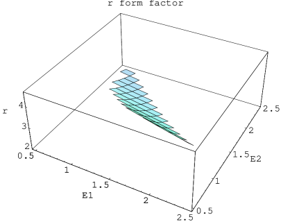
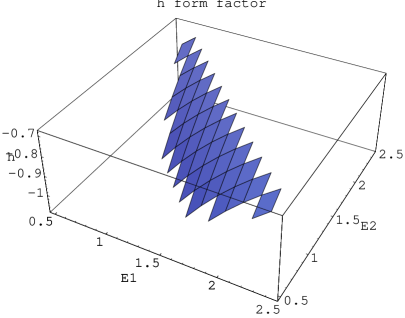
(a)                                                                       (b)

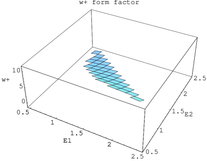
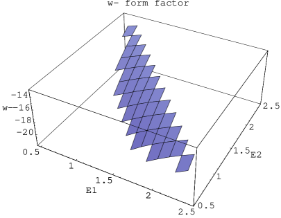
(c)                                                                       (d)

Figure 2: The relevant form factors for $B^{-}\to\pi^{+}\pi^{-}$ semileptonic decay at $s=5$ GeV² as a function of $E_{1}$ and $E_{2}$. Units are GeV^-1 for $w_{+}$ in (c), $w_{-}$ in (d) and $r$ in (a), GeV^-3 for $h$ in (b).

A different way to present the data is to introduce averaged form factors. We choose to perform an average in the pion energies according to the following formula:

$$f(s)=\frac{1}{\Delta(s)}\int_{s/(2m_{B})}^{m_{B}/2}dE_{2}~{}\int_{s/(4E_{2})}^{(s+m_{B}^{2})/(2m_{B})-E_{2}}dE_{1}~{}f(s,~{}E_{1},E_{2})~{},$$ (28)

valid for all the form factors ($f=h,~{}r,~{}w_{+},~{}w_{-}$). Here $\Delta(s)$ is the allowed area in the $(E_{1},~{}E_{2})$ plane:

$$\Delta(s)=\frac{m_{B}^{4}-s^{2}}{8m_{B}^{2}}+\frac{s}{4}\ln\frac{s}{m_{B}^{2}}~{}.$$ (29)

The numerical results we obtain have an average error around $10\%$. A simple way to present the data is by an analytical formula: for example the data can be fitted by the following relation

$$f(s)~{}=~{}\frac{\beta~{}(s-s_{1})~{}(s-s_{2})}{(s-s_{3})^{2}~{}+~{}s_{4}^{2}}~{},$$ (30)

a procedure which introduces an average numerical error of $\pm 10\%$; we stress, however that in computing the width we have not used this fit and therefore this further error has not been introduced. We also point out that the Breit-Wigner shape of eq. (30) is a useful parameterization and has no dynamical meaning.

The values of the coefficients $s_{k}~{},\beta$ appearing in (30) are reported in table 5 for all the form factors of the $B^{-}$ decay. The form factors are depicted in figs. 3. We observe that due to the limitations of our approach, the kinematical region of validity of the present model has no overlap with the soft pion region where pole diagrams, see e.g. [2], are expected to dominate. Therefore a comparison of our work with the results of these models is impossible.

(a)                                                                       (b)

(c)                                                                       (d)

Figure 3: The averaged form factors for $B^{-}\to\pi^{+}\pi^{-}$ semileptonic decay. Units are GeV^-1 for $w_{+}$ in (c), $w_{-}$ in (d) and $r$ in (a), GeV^-3 for $h$ in (b).

Let us now evaluate the partial width $\Gamma(B\to\pi\pi\ell\nu)$. The relevant formulae to compute the width are reported in [2] and we do not reproduce them here. We only give our numerical results for the cut-off width ($s\geq 1{\rm GeV}^{2}$). Numerically we get

$${\cal BR}(B^{-}\to\pi^{+}\pi^{-}\ell^{-}\bar{\nu}_{\ell})=2.2\ \left(\frac{|V_{ub}|}{3.2\times 10^{-3}}\right)^{2}\times 10^{-4}~{}{\hskip 28.45274pt}~{}(s\geq 1{\rm GeV}^{2})~{}.$$ (31)

For the other decay channel we have:

$${\cal BR}(\bar{B}^{0}\to\pi^{+}\pi^{0}\ell^{-}\bar{\nu}_{\ell})=3.2\ \left(\frac{|V_{ub}|}{3.2\times 10^{-3}}\right)^{2}\times 10^{-4}~{}~{}{\hskip 28.45274pt}~{}(s\geq 1{\rm GeV}^{2})~{}.$$ (32)

The contribution of the $\rho$ resonance to these decay modes can be estimated in the present model [9] as follows:

$${\cal BR}(B^{-}\to\pi^{+}\pi^{-}\ell^{-}\bar{\nu}_{\ell})\Big{|}_{\rho}=1.2\ \left(\frac{|V_{ub}|}{3.2\times 10^{-3}}\right)^{2}\times 10^{-4}~{}.$$ (33)

For the other decay channel we have:

$${\cal BR}(\bar{B}^{0}\to\pi^{+}\pi^{0}\ell^{-}\bar{\nu}_{\ell})\Big{|}_{\rho}=2.4\ \left(\frac{|V_{ub}|}{3.2\times 10^{-3}}\right)^{2}\times 10^{-4}~{}.$$ (34)

This latter branching ratio is in agreement with the experimental figure quoted above.

We can therefore conclude that from an experimental point of view the semileptonic decay channel with two non-resonant pions in the final state represents an interesting process with a significant branching ratio, of the same order of magnitude of the single pion or the single $\rho$ semileptonic decay mode. It would be nice to find this decay mode in the future experimental analysis and to test the present prediction of the QCD relativistic potential model.

Acknowledgements. We wish to thank P. Colangelo, F. De Fazio, M. Pellicoro and A. D. Polosa for useful comments.

Table 1: Numerical values of the form factors for several values of $E_{1}~{}$, $~{}E_{2}$ (in GeV) and $s~{}=~{}1$ GeV². Units are GeV${}^{-1}~{}$ ($r$, $w_{+}$ and $w_{-}$ ) and GeV${}^{-3}~{}$ ($h$).

$(E_{1},~{}E_{2})~{}$	$r$	$h$	$w_{+}$	$w_{-}$
$~{}(0.14~{},~{}2.36)~{}$	$-~{}0.26$	0.53	5.99	3.12
$~{}(0.18~{},~{}2.07)~{}$	$-~{}0.23$	0.62	5.89	2.83
$~{}(0.23~{},~{}1.79)~{}$	$-~{}0.16$	0.73	5.89	2.44
$~{}(0.28~{},~{}1.51)~{}$	$-~{}0.039$	0.88	5.77	1.92
$~{}(0.35~{},~{}1.23)~{}$	$~{}0.18$	1.07	5.60	1.28
$~{}(0.43~{},~{}0.94)~{}$	$~{}0.56$	1.32	5.41	0.56
$~{}(0.57~{},~{}0.66)~{}$	$~{}1.22$	1.60	5.18	- 0.019
$~{}(0.85~{},~{}0.38)~{}$	$~{}2.21$	1.72	4.20	0.58

Table 2: Numerical values of the form factors for several values of $E_{1}~{}$, $~{}E_{2}$ (in GeV) and $s=5$ GeV². Units are GeV${}^{-1}~{}$ ($r$, $w_{+}$ and $w_{-}$ ) and GeV${}^{-3}~{}$ ($h$).

$(E_{1},~{}E_{2})~{}$	$r$	$h$	$w_{+}$	$w_{-}$
$~{}(0.54~{},~{}2.40)$	2.15	- 0.76	- 1.25	- 13.9
$~{}(0.62~{},~{}2.16)$	2.36	- 0.84	- 0.31	- 15.1
$~{}(0.71~{},~{}1.92)$	2.60	- 0.92	0.85	- 16.5
$~{}(0.82~{},~{}1.68)$	2.88	- 0.99	2.27	- 17.9
$~{}(0.96~{},~{}1.44)$	3.22	- 1.06	3.98	- 19.3
$~{}(1.14~{},~{}1.20)$	3.62	- 1.10	6.01	- 20.7
$~{}(1.40~{},~{}0.95)$	4.08	- 1.08	8.29	- 21.5
$~{}(1.82~{},~{}0.71)$	4.52	- 0.95	10.5	- 20.9

Table 3: Numerical values of the form factors for several values of $E_{1}~{}$, $~{}E_{2}$ (in GeV) and $s=10$ GeV². Units are GeV${}^{-1}~{}$ ($r$, $w_{+}$ and $w_{-}$ ) and GeV${}^{-3}~{}$ ($h$).

$(E_{1},~{}E_{2})~{}$	$r$	$h$	$w_{+}$	$w_{-}$
$~{}(1.03~{},~{}2.45)~{}$	0.42	- 0.29	- 2.71	- 0.36
$~{}(1.13~{},~{}2.26)~{}$	0.29	- 0.32	- 2.71	- 0.33
$~{}(1.24~{},~{}2.08)~{}$	0.14	- 0.34	- 2.68	- 0.37
$~{}(1.37~{},~{}1.89)~{}$	- 0.044	- 0.37	- 2.60	- 0.49
$~{}(1.52~{},~{}1.70)~{}$	- 0.24	- 0.40	- 2.42	- 0.75
$~{}(1.70~{},~{}1.51)~{}$	- 0.45	- 0.42	- 2.11	- 1.15
$~{}(1.93~{},~{}1.32)~{}$	- 0.63	- 0.44	- 1.60	- 1.78
$~{}(2.23~{},~{}1.13)~{}$	- 0.75	- 0.44	- 0.81	- 2.72

Table 4: Numerical values of the form factors for several values of $E_{1}~{}$, $~{}E_{2}$ (in GeV) and $s=19$ GeV². Units are GeV${}^{-1}~{}$ ($r$, $w_{+}$ and $w_{-}$ ) and GeV${}^{-3}~{}$ ($h$).

$(E_{1},~{}E_{2})~{}$	$r$	$h$	$w_{+}$	$w_{-}$
$~{}(1.87~{},~{}2.55)~{}$	- 0.81	0.0041	- 1.31	1.73
$~{}(1.94~{},~{}2.45)~{}$	- 0.87	0.0028	- 1.37	1.77
$~{}(2.02~{},~{}2.36)~{}$	- 0.95	0.0012	- 1.44	1.80
$~{}(2.10~{},~{}2.27)~{}$	- 1.02	0.00092	- 1.51	1.82
$~{}(2.19~{},~{}2.17)~{}$	- 1.10	-  0.0033	- 1.57	1.83
$~{}(2.29~{},~{}2.08)~{}$	- 1.18	-  0.0062	- 1.64	1.83
$~{}(2.40~{},~{}1.99)~{}$	- 1.27	-  0.0096	- 1.70	1.81
$~{}(2.51~{},~{}1.89)~{}$	- 1.35	-  0.014	- 1.75	1.77

Table 5: Numerical values of the parameters appearing in the formula $\displaystyle{f(s)~{}=~{}\frac{\beta~{}(s-s_{1})~{}(s-s_{2})}{(s-s_{3})^{2}~{}+~{}s_{4}^{2}}}~{}$. $f(s)$ is any of the averaged form factors.  Units are GeV${}^{2}~{}$ for $s_{1}~{}$, $s_{2}~{}$, $s_{3}~{}$ and $s_{4}$; $f(s)$ and $\beta$ have the same units.

form factor	$s_{1}$	$s_{2}$	$s_{3}$	$s_{4}^{2}$	$\beta$
$~{}w_{+}~{}$	$-~{}0.957$	$+~{}7.15$	$+~{}3.98$	$+~{}3.38$	$-~{}1.87$
$~{}w_{-}~{}$	$+~{}1.77$	$+~{}11.4$	$+~{}4.20$	$+~{}3.47$	$+~{}3.91$
$~{}h~{}$	$+~{}3.25$	$+~{}19.5$	$+~{}5.38$	$+~{}7.93$	$+~{}0.207$
$~{}r~{}$	$-~{}0.446$	$+~{}9.47$	$+~{}4.32$	$+~{}11.5$	$-~{}1.57$

References

- [1] The BaBar Physics Book, edited by P. F. Harrison and H. R. Quinn, SLAC-R-504 (1998).
- [2] C. L. Y. Lee, M. Lu and M.B. Wise, Phys. Rev. D 46 (1992) 5040.
- [3] G. Burdman, J. F. Donoghue Phys. Lett. B 280 (1992) 287.
- [4] M. B. Wise, Phys. Rev. D 45, (1992) 2188.
- [5] L. Wolfenstein, Phys. Lett. B 291 (1992) 177.
- [6] R. Casalbuoni, A. Deandrea, N. Di Bartolomeo, F. Feruglio, R. Gatto, G. Nardulli, Phys. Lett. B 299 (1993) 139; Phys. Rep. 281 (1997) 145.
- [7] P. Cea, P. Colangelo, L. Cosmai and G. Nardulli, Phys. Lett. B 206 (1988) 691; P. Colangelo, G. Nardulli and M. Pietroni, Phys. Rev. D 43 (1991) 3002.
- [8] G. Nardulli, T. N. Pham, Phys. Lett. B 391 (1997) 165; J. F. Donoghue, Eugene Golowich, Alexey A. Petrov, Phys. Rev. D 55 (1997) 2657.
- [9] P. Colangelo, F. De Fazio, M. Ladisa, G. Nardulli, P. Santorelli, A. Tricarico, Eur. Phys. J. C 8 (1999) 81.
- [10] M. Ladisa, G. Nardulli and P. Santorelli, Phys. Lett. B 455 (1999) 283.
- [11] J.L. Richardson, Phys. Lett. B 82 (1979) 272.
- [12] E. E. Salpeter, Phys. Rev. 87 (1952) 328.