Abstract

We compute the helicity skewed quark distributions $\widetilde{H}$ and $\widetilde{E}$ in the chiral quark-soliton model of the nucleon. This model emphasizes correctly the role of spontaneously broken chiral symmetry in structure of nucleon. It is based on the large-$N_{c}$ picture of the nucleon as a soliton of the effective chiral lagrangian and allows to calculate the leading twist quark– and antiquark distributions at a low normalization point.

We discuss the role of chiral symmetry in the helicity skewed quark distributions $\widetilde{H}$ and $\widetilde{E}$. We show that generalization of soft pion theorems, based on chiral Ward identities, leads in the region of $-\xi<x<\xi$ to the pion pole contribution to $\widetilde{E}$ which dominates at small momentum transfer.

1 Introduction

Recently, a new type of parton distributions [1, 2, 3, 4] has attracted considerable interest, the so-called skewed parton distributions (SPD’s), which are generalizations simultaneously of the usual parton distributions, distribution amplitudes and of the elastic nucleon form factors (for review see [5]). Taking the $n$–th moment of the SPD’s one obtains the form factors (i.e., non-forward matrix elements) of the spin–$n$, twist–two quark and gluon operators. On the other hand, in the forward limit the SPD’s reduce to the usual quark, antiquark and gluon distributions. In other words, the SPD’s interpolate between the traditional inclusive (parton distributions) and exclusive (form factors) characteristics of the nucleon and thus provide us with a considerable new amount of information on nucleon structure.

The SPD’s are not accessible in standard inclusive measurements. They can, however, be measured in deeply–virtual Compton scattering (DVCS) and in hard exclusive leptoproduction of mesons. The very possibility to probe SPD’s in these reactions is due to QCD factorization theorem of Ref. [4]. Feasibility of experimental measurements of SPD’s in hard exclusive reactions is currently being studied [6, 7, 8, 9]. A quantitative description of these classes of processes requires non-perturbative information in the form of the SPD’s at some initial normalization point. Although the skewed parton distributions can be reduced in certain limiting cases to already known quantities (parton distributions, form factors), even their qualitative behaviour is unknown to large extent. That is why model calculations of these quantities are of big importance. There were already model calculations of SPD’s: in the bag model [10] and in the chiral quark-soliton model [11]. In the latter calculation a drastic variation of flavour singlet $H(x,\xi,t)$ at $x$ near $x=|\xi|$ was observed. Such behaviour is related to the fact that the SPD’s in the region $-\xi<x<\xi$ have properties of distribution amplitudes. This feature, being very important for the understanding of SPD’s, requires a field theoretic description of nucleon’s constituents and that is the reason why it can not by reproduced in the bag model.

Our aim now is to compute helicity skewed quark distributions of the nucleon using the methods of ref. [11]. We shall see that generalization of low energy theorems requires that the skewed distribution $\widetilde{E}$ develops a pion pole at $\Delta^{2}=m_{\pi}^{2}$ of the form:

$$\lim_{\Delta^{2}\to m_{\pi}^{2}}\widetilde{E}^{(3)}_{\pi}(x,\xi,\Delta^{2})=-\frac{4g_{A}M_{N}^{2}}{|\xi|(\,\Delta^{2}-m_{\pi}^{2}\,)}\,\theta\Big{(}|x|<|\xi|\Big{)}\ \Phi_{\pi}\Biggl{(}\frac{x}{\xi}\Biggr{)},$$ (1.1)

where $\Phi_{\pi}(z)$ is distribution amplitude of the pion. In refs. [9, 13] it was shown that this contribution to $\widetilde{E}$ leads to considerable enhancement of the amplitude of hard exclusive production of charged pions and to large azimuthal spin asymmetry in exclusive $\pi^{\pm}$ production [13].

We shall see that in the chiral quark-soliton model the pion pole contribution is related to the large distance asymptotic of the pion mean-field, which is controlled by PCAC.

2 Definition of skewed helicity quark distributions

In QCD the helicity skewed quark distributions are defined through non-diagonal matrix elements of product of quark fields at light–cone separation. Here and in the following, we shall use the notations of ref. [5]

$$\int\frac{d\lambda}{2\pi}e^{i\lambda x}\langle P^{\prime}|\bar{\psi}_{f}(-\lambda n/2){\hat{n}}\gamma_{5}\psi_{f}(\lambda n/2)|P\rangle = \widetilde{H}_{f}(x,\xi,\Delta^{2})\;\bar{U}(P^{\prime})\;\hat{n}\gamma_{5}\;U(P)$$

$$+ \frac{1}{2M_{N}}\;\widetilde{E}_{f}(x,\xi,\Delta^{2})\;\bar{U}(P^{\prime})\;(n\cdot\Delta)\gamma_{5}U(P).$$

Here $n_{\mu}$ is a light-cone vector,

$$n^{2} = 0,\hskip 42.67912ptn\cdot(P+P^{\prime})=2\ n\cdot\bar{P}\;=\;\;2,$$ (2.3)

$\Delta$ is the four–momentum transfer,

$$\Delta=P^{\prime}-P,$$ (2.4)

$M_{N}$ denotes the nucleon mass, and $U(P)$ is a standard Dirac spinor. The skewed quark distributions, $\widetilde{H}(x,\xi,\Delta^{2})$ and $\widetilde{E}(x,\xi,\Delta^{2})$, are regarded as functions of the variable $x$, the square of the four–momentum transfer, $\Delta^{2}=t$, and its longitudinal component

$$\xi=-\frac{1}{2}\,(n\cdot\Delta).$$ (2.5)

In the forward case, $P=P^{\prime}$, both $\Delta$ and $\xi$ are zero, and the second term on the r.h.s. of eq.(LABEL:E-H-QCD-2) disappears. In this limit the function $\widetilde{H}$ becomes the usual polarised parton distribution function,

$$\widetilde{H}_{f}\Big{(}x,\xi=0,\Delta^{2}=0\Big{)} = \left\{\begin{array}[]{cr}\Delta q_{f}(x),&\hskip 14.22636ptx\;>\;0\,,\\ \Delta\bar{q}_{f}(-x),&\hskip 14.22636ptx\;<\;0\,.\end{array}\right.$$ (2.8)

On the other hand, taking the first moment of eq.(LABEL:E-H-QCD-2) one reduces the operator on the l.h.s. to the local axial vector current. The dependence of $\widetilde{H}$ and $\widetilde{E}$ on $\xi$ disappears, and the functions reduce to the usual axial form factors of the nucleon,

$$\int_{-1}^{1}dx\;\widetilde{H}(x,\xi,\Delta^{2}) = G_{A}(\Delta^{2}),$$ (2.9)

$$\int_{-1}^{1}dx\;\widetilde{E}(x,\xi,\Delta^{2}) = G_{P}(\Delta^{2}).$$ (2.10)

Taking higher moments of the distribution functions one obtains the form factors of the twist–2, spin–$n$ operators.

3 Chiral quark–soliton model of the nucleon

Recently a new approach to the calculation of quark distribution functions of the nucleon has been developed [14] in the framework of the chiral quark-soliton model of the nucleon [15]. In present paper we apply this approach to the calculation of skewed quark distributions. It is essentially based on the $1/N_{c}$ expansion. Although in reality the number of colours $N_{c}=3$, the academic limit of large $N_{c}$ is known to be a useful guideline. At large $N_{c}$ the nucleon is heavy and can be viewed as a classical soliton of the pion field [16, 17]. In this paper we work with the effective chiral action given by the functional integral over quarks in the background pion field [18, 19, 20]:

$$\exp\Big{(}iS_{{\rm eff}}[\pi(x)]\Big{)}=\int D\psi D\bar{\psi}\;\exp\left(i\int d^{4}x\,\bar{\psi}(i\hat{\partial}-MU^{\gamma_{5}})\psi\right),$$

$$U\;=\;\exp\Big{(}i\pi^{a}(x)\tau^{a}\Big{)},\hskip 28.45274ptU^{\gamma_{5}}\;=\;\exp\Big{(}i\pi^{a}(x)\tau^{a}\gamma_{5}\Big{)}\;=\;\frac{1+\gamma_{5}}{2}U+\frac{1-\gamma_{5}}{2}U^{\dagger}.$$ (3.11)

Here $\psi$ is the quark field, $M$ is the effective quark mass, which is due to the spontaneous breakdown of chiral symmetry (generally speaking, it is momentum dependent), and $U$ is the $SU(2)$ chiral pion field. The effective chiral action given by (3.11) is known to contain automatically the Wess–Zumino term and the four-derivative Gasser–Leutwyler terms, with correct coefficients. The equation (3.11) has been derived from the instanton model of the QCD vacuum [20, 21], which provides a natural mechanism of chiral symmetry breaking and enables one to express the dynamical mass $M$ and the ultraviolet cutoff intrinsic in (3.11) through the $\Lambda_{QCD}$ parameter. The ultraviolet regularization of the effective theory is provided by the specific momentum dependence of the mass, $M(p^{2})$, which drops to zero for momenta of order of the inverse instanton size in the instanton vacuum, $1/\rho\sim 600\,{\rm MeV}$. For simplicity we shall neglect this momentum dependence in the general discussion; it will be taken into account again in the theoretical analysis and in the numerical estimates later.

An immediate application of the effective chiral theory (3.11) is the quark-soliton model of baryons of ref. [15], which is in the spirit of the earlier works [22, 23]. According to this model nucleons can be viewed as $N_{c}$ “valence” quarks bound by a self-consistent pion field (the “soliton”) whose energy coincides with the aggregate energy of the quarks of the negative-energy Dirac continuum. Similarly to the Skyrme model large $N_{c}$ is needed as a parameter to justify the use of the mean-field approximation; however, the $1/N_{c}$–corrections can be — and, in some cases, have been — computed [24].

Let us remind the reader how the nucleon is described in the effective low-energy theory (3.11). Integrating out the quarks in (3.11) one finds the effective chiral action,

$$S_{{\rm eff}}[\pi^{a}(x)]=-N_{c}\,\mbox{Sp}\log D(U)\,,\hskip 28.45274ptD(U)\;\;=\;\;i\partial_{0}-H(U),$$ (3.12)

where $H(U)$ is the one-particle Dirac Hamiltonian,

$$H(U)=-i\gamma^{0}\gamma^{k}\partial_{k}+M\gamma^{0}U^{\gamma_{5}}\,,$$ (3.13)

and $\mbox{Sp}\ldots$ denotes the functional trace. For a given time-independent pion field $U=\exp(i\pi^{a}({\bf x})\tau^{a})$ one can determine the spectrum of the Dirac Hamiltonian,

$$H\Phi_{n}=E_{n}\Phi_{n}.$$ (3.14)

It contains the upper and lower Dirac continua (distorted by the presence of the external pion field), and, in principle, also discrete bound-state level(s), if the pion field is strong enough. If the pion field has unity winding number, there is exactly one bound-state level which travels all the way from the upper to the lower Dirac continuum as one increases the spatial size of the pion field from zero to infinity [15]. We denote the energy of the discrete level as $E_{{\rm lev}},\;\;-M\leq E_{{\rm lev}}\leq M$. One has to occupy this level to get a non-zero baryon number state. Since the pion field is colour blind, one can put $N_{c}$ quarks on that level in the antisymmetric state in colour.

The limit of large $N_{c}$ allows us to use the mean-field approximation to find the nucleon mass. To get the nucleon mass one has to add $N_{c}E_{{\rm lev}}$ and the energy of the pion field. Since the effective chiral lagrangian is given by the determinant (3.12) the energy of the pion field coincides exactly with the aggregate energy of the lower Dirac continuum, the free continuum subtracted. The self-consistent pion field is thus found from the minimisation of the functional [15]

$$M_{N}=\min_{U}\;N_{c}\left\{E_{{\rm lev}}[U]\;+\;\sum_{E_{n}<0}\Big{(}E_{n}[U]-E_{n}^{(0)}\Big{)}\right\}.$$ (3.15)

From symmetry considerations one looks for the minimum in a hedgehog ansatz:

$$U_{c}({\bf x})\;=\;\exp\Big{(}i\pi^{a}({\bf x})\tau^{a}\Big{)}\;=\;\exp\Big{(}in^{a}\tau^{a}P(r)\Big{)},\hskip 28.45274ptr\;=\;|{\bf x}|,\hskip 28.45274pt{\bf n}\;=\;\frac{{\bf x}}{r},$$ (3.16)

where $P(r)$ is called the profile of the soliton.

The minimum of the energy (3.15) is degenerate with respect to translations of the soliton in space and to rotations of the soliton field in ordinary and isospin space. For the hedgehog field (3.16) the two rotations are equivalent. The projection on a nucleon state with given spin ($S_{3}$) and isospin ($T_{3}$) components is obtained by integrating over all spin-isospin rotations, $R$ [17, 15],

$$\langle S=T,S_{3},T_{3}|\ldots|S=T,S_{3},T_{3}\rangle = \int dR\;\phi^{\ast\;S=T}_{S_{3}T_{3}}(R)\;\ldots\;\phi^{S=T}_{S_{3}T_{3}}(R)\,.$$ (3.17)

Here $\phi^{S=T}_{S_{3}T_{3}}(R)$ is the rotational wave function of the nucleon given by the Wigner finite-rotation matrix [17, 15]:

$$\phi_{S_{3}T_{3}}^{S=T}(R) = (-1)^{T+T_{3}}\sqrt{2S+1}\,D_{-T_{3},S_{3}}^{\,S=T}(R).$$ (3.18)

Analogously, the projection on a nucleon state with given momentum ${\bf P}$ is obtained by integrating over all shifts, ${\bf X}$, of the soliton,

$$\langle{\bf P^{\prime}}|\ldots|\ {\bf P}\rangle = \int d^{3}{\bf X}\;e^{i\left({\bf P^{\prime}-P}\right)\cdot{\bf X}}\;\ldots$$ (3.19)

4 Skewed quark distributions in the chiral quark–soliton model

We now turn to the calculation of the skewed quark distributions in the chiral quark–soliton model. This description of the nucleon is based on the $1/N_{c}$-expansion. At large $N_{c}$ the nucleon is heavy — its mass is $O(N_{c})$. For the large-$N_{c}$ nucleon eq. (LABEL:E-H-QCD-2) simplifies as follows:

$$\int\frac{d\lambda}{2\pi}e^{i\lambda x}\langle P^{\prime},S_{3}^{\prime}|\bar{\psi}_{f}(-\lambda n/2){\hat{n}}\gamma_{5}\psi_{f}(\lambda n/2)|P,S_{3}\rangle$$

$$\,=\,\frac{\tau^{3}_{ff}}{2}\Bigg{\{}\,2\delta^{3i}\widetilde{H}_{f}(x,\xi,t) - \frac{\Delta^{3}\Delta^{i}}{2M_{N}^{2}}\,\widetilde{E}_{F}(x,\xi,t)\,\Bigg{\}}\,\sigma^{i}_{S_{3}^{\prime}S_{3}}\,,$$ (4.20)

where $S_{3},S_{3}^{\prime}$ denote the projections of the nucleon spin. From this expression we immediately see that in the leading order of the $1/N_{c}$-expansion only the flavour isovector part of

$$\widetilde{H}^{(3)}(x,\xi,\Delta^{2})=\widetilde{H}_{u}(x,\xi,\Delta^{2})-\widetilde{H}_{d}(x,\xi,\Delta^{2})$$

and

$$\widetilde{E}^{(3)}(x,\xi,\Delta^{2})=\widetilde{E}_{u}(x,\xi,\Delta^{2})-\widetilde{E}_{d}(x,\xi,\Delta^{2})$$

are non-zero. The isosinglet part of $\widetilde{H}(x,\xi,\Delta^{2})$ and the isosinglet part of $\widetilde{E}(x,\xi,\Delta^{2})$ appear only in the next–to–leading order of the $1/N_{c}$–expansion, i.e., after taking into account the finite angular velocity of the soliton rotation.

Before computing the skewed quark distribution functions we must determine the parametric order in $1/N_{c}$ of the kinematical variables involved. Generally, when describing parton distributions in the large–$N_{c}$ limit, one has $x\sim 1/N_{c}$, since the nucleon momentum is distributed among $N_{c}$ quarks. Furthermore, as in the calculation of nucleon form factors we consider momentum transfers to be of order $t\sim N_{c}^{0}$; hence, in particular, $\xi\sim 1/N_{c}$, so that $\xi$ is of the same parametric order as $x$.

Technically the calculation of the skewed parton distributions proceeds in much the same way as that of the usual parton distributions [14, 11]. Using the formalism developed in [14, 11] we obtain:

$$\widetilde{H}^{(3)}(x,\xi,\Delta^{2})\,= - \frac{N_{c}M_{N}}{6\pi\mbox{\boldmath$\Delta$}_{\perp}^{2}}\int dz^{0}\int d^{3}{\bf X}\,\exp\Big{(}i\mbox{{\boldmath$\Delta$}}\cdot{\bf X}\Big{)}\sum\limits_{{\scriptstyle}\atop{\scriptstyle{\rm occup.}}}\exp\Big{(}iz^{0}\Big{[}(x+\xi)M_{N}-E_{n}\Big{]}\Big{)}\;$$ (4.21)

$$\Phi_{n}^{\dagger}({\bf X})\Big{(}\mbox{\boldmath$\Delta$}_{\perp}^{2}\tau^{3}+2\xi M_{N}\mbox{{\boldmath$\Delta$}}_{\perp}\cdot\mbox{\boldmath$\tau$}_{\perp}\Big{)}\Big{(}1+\gamma^{0}\gamma^{3}\Big{)}\gamma_{5}\,\Phi_{n}\,({\bf X}-z^{0}{\bf e}_{3}),$$

$$\widetilde{E}^{(3)}(x,\xi,\Delta^{2})\,= - \frac{N_{c}M_{N}^{2}}{3\pi\xi\mbox{\boldmath$\Delta$}_{\perp}^{2}}\int dz^{0}\int d^{3}{\bf X}\,\exp\Big{(}i\mbox{{\boldmath$\Delta$}}\cdot{\bf X}\Big{)}\sum\limits_{{\scriptstyle}\atop{\scriptstyle{\rm occup.}}}\exp\Big{(}iz^{0}\Big{[}(x+\xi)M_{N}-E_{n}\Big{]}\Big{)}$$ (4.22)

$$\Phi_{n}^{\dagger}({\bf X})\Big{(}\mbox{{\boldmath$\Delta_{\perp}$}}\cdot\mbox{{\boldmath$\tau_{\perp}$ }}\Big{)}\Big{(}1+\gamma^{0}\gamma^{3}\Big{)}\gamma_{5}\,\Phi_{n}\,({\bf X}-z^{0}{\bf e}_{3}).$$

Before going ahead with the evaluation of the expressions eqs.(4.21, 4.22) we would like to demonstrate that the two limiting cases of the skewed distributions — usual parton distributions and elastic form factors — are correctly reproduced within the chiral quark–soliton model. Taking in eq.(4.21) the forward limit, $\Delta\rightarrow 0$, one recovers the formula for the usual polarized (anti–) quark distributions in our model which was obtained in ref. [14]. Thus the forward limit, eq. (2.8), is reproduced. On the other hand, integrating eq. (4.21) over $-1\leq x\leq 1$ one obtains (up to corrections parametrically small in $1/N_{c}$) the expressions for the axial form factors of the nucleon derived in ref. [25]:

$$\int_{-1}^{1}dx\ \widetilde{H}^{(3)}(x,\xi,\Delta^{2}) = -\frac{N_{c}}{3}\int d^{3}{\bf X}\,\exp\Big{(}i\mbox{{\boldmath$\Delta$}}\cdot{\bf X}\Big{)}\sum\limits_{{\scriptstyle}\atop{\scriptstyle{\rm occup.}}}\Phi_{n}^{\dagger}({\bf X})\,\tau^{3}\gamma^{0}\gamma^{3}\gamma_{5}\,\Phi_{n}\,({\bf X})$$ (4.23)

$$= G_{A}^{\rm(T=1)}(\Delta^{2})\,.$$

Actually experimental $G_{A}^{\rm(T=1)}(\Delta^{2})$ is very well reproduced in the chiral quark-soliton model up to momenta of order $\Delta^{2}\sim 1$ GeV² [24].

Now if one integrates eq. (4.22) over $-1\leq x\leq 1$ one obtains (up to corrections parametrically small in $1/N_{c}$) the following expression:

$$\int_{-1}^{1}dx\,\widetilde{E}^{(3)}(x,\xi,\Delta^{2})=-\frac{2N_{c}M_{N}}{3\xi\mbox{\boldmath$\Delta$}_{\perp}^{2}}\int d^{3}{\bf X}\exp\Big{(}i\mbox{{\boldmath$\Delta$}}\cdot{\bf X}\Big{)}\sum\limits_{{\scriptstyle}\atop{\scriptstyle{\rm occup.}}}\Phi_{n}^{\dagger}({\bf X})\gamma^{0}\gamma^{3}\Big{(}\mbox{{\boldmath$\Delta_{\perp}$}}\cdot\mbox{{\boldmath$\tau_{\perp}$}}\Big{)}\gamma_{5}\Phi_{n}({\bf X}).$$ (4.24)

Using the “hedgehog” symmetry of the pion mean-field one can easily show that the expression (4.24) is a function of only $\Delta^{2}$ and coincides with expression for pseudoscalar nucleon form factor in the chiral quark soliton model, see e.g. ref. [24].

Eqs. (4.21, 4.22) express the SPD’s as a sum over quark single–particle levels in the soliton field. This sum runs over all occupied levels, including both the discrete bound–state level and the negative Dirac continuum. We remind the reader that in the case of usual parton distributions it was demonstrated that in order to ensure the positivity of the antiquark distributions it is essential to take into account the contributions of all occupied levels of the Dirac Hamiltonian [14]. We shall see below that also in the case of skewed quark distributions the contribution of the Dirac continuum drastically changes the shape of the distribution function. That is especially important to reproduce the pion pole contribution to the spin-flip SPD $\widetilde{E}^{(3)}$ required by chiral Ward identities.

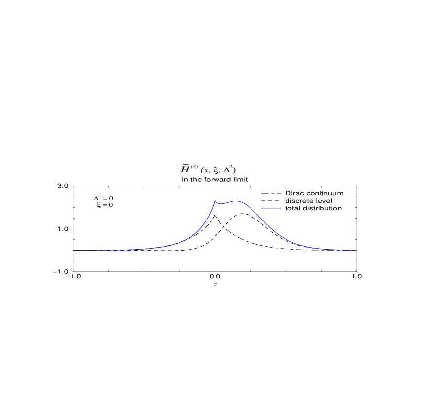
Figure 1: The isovector distribution $\widetilde{H}(x,\xi,\Delta^{2})$ in the forward limit, $\Delta=0$. Dashed line: contribution from the discrete level. Dashed-dotted line: contribution from the Dirac continuum according to the interpolation formula, eq. (4). Solid line: total distribution (sum of the dashed and dashed-dotted curves).

The contribution of the discrete bound–state level to eqs. (4.21, 4.22) can be computed using the expressions given in the Appendix. The result is shown in Figs. 1 for the forward case and Figs. 2 for a non-zero momentum transfer. Being taken by itself this contribution resembles qualitatively the shape of SPD’s $\widetilde{H}$ and $\widetilde{E}$ obtained in the bag model [10].

To calculate the contribution of the Dirac continuum to eqs. (4.21, 4.22) we resort to an approximation which proved to be very successful in the computation of usual parton distributions, the so–called interpolation formula [14]. One first expresses the continuum contribution as a functional trace involving the quark propagator in the background pion field. The quark propagator can then be expanded in powers of the formal parameter $\partial U/(-\partial^{2}+M^{2})$, which becomes small in three limiting cases: i) low momenta, $|\partial U|\ll M$, ii) high momenta, $|\partial U|\gg M$, iii) any momenta but small pion fields, $|\log U|\ll 1$. One may therefore expect that this approximation has good accuracy also in the general case. As was shown in refs. [14] for usual parton distributions this approximation preserves the positivity of the antiquark distributions and all sum rules; moreover, it gives results very close to those obtained by exact numerical diagonalisation of the Dirac Hamiltonian and summation over the negative–energy levels.

Simple generalization of the technique developed in [14, 11] allows us to express the Dirac continuum contribution to the SPD’s directly in terms of pion mean-field (3.16):

$$\widetilde{H}^{(3)}(x,\xi,\Delta^{2})_{\rm cont} = -\frac{M_{N}N_{c}}{3\ \mbox{\boldmath$\Delta$}_{\perp}^{2}}\;\mbox{Im}\,\int\frac{d^{3}k}{(2\pi)^{3}}\int\frac{d^{4}p}{(2\pi)^{4}}\;\delta\left[\Bigl{(}x-\xi\Bigr{)}M_{N}-v\cdot p\right]$$

$$\times \frac{M_{1}^{1/2}}{\Big{(}p_{1}^{2}-M_{1}^{2}+i0\Big{)}}\,\frac{M_{2}^{3/2}}{\Big{(}p_{2}^{2}-M_{2}^{2}+i0\Big{)}}\Big{(}k\cdot v+\frac{1}{2}\Delta\cdot v\Big{)}$$

$$\times \mbox{Tr}_{\rm fl.}\Biggl{[}\Big{(}\mbox{\boldmath$\Delta$}_{\perp}^{2}\tau^{3}+2\xi M_{N}\mbox{{\boldmath$\Delta_{\perp}$}}\cdot\mbox{{\boldmath$\tau_{\perp}$}}\Big{)}\widetilde{U}\Big{(}{\bf k-}\mbox{{\boldmath$\frac{\Delta}{2}$}}\Big{)}\Big{[}\widetilde{U}\Big{(}{\bf k+}\mbox{{\boldmath$\frac{\Delta}{2}$}}\Big{)}\Big{]}^{+}\Biggr{]}$$

$$+ \Biggl{(}\xi\to-\xi,\;\;\mbox{{\boldmath$\Delta$}}\to-\mbox{{\boldmath$\Delta$}}\Biggr{)},$$

$$\widetilde{E}^{(3)}(x,\xi,\Delta^{2})_{\rm cont} = -\frac{2M_{N}^{2}N_{c}}{3\ \xi\ \mbox{\boldmath$\Delta$}_{\perp}^{2}}\;\mbox{Im}\,\int\frac{d^{3}k}{(2\pi)^{3}}\int\frac{d^{4}p}{(2\pi)^{4}}\;\delta\left[\Bigl{(}x-\xi\Bigr{)}M_{N}-v\cdot p\right]$$

$$\times \frac{M_{1}^{1/2}}{\Big{(}p_{1}^{2}-M_{1}^{2}+i0\Big{)}}\,\frac{M_{2}^{3/2}}{\Big{(}p_{2}^{2}-M_{2}^{2}+i0\Big{)}}\,\Big{(}k\cdot v+\frac{1}{2}\Delta\cdot v\Big{)}$$

$$\times \mbox{Tr}_{\rm fl.}\Biggl{[}\Big{(}\mbox{{\boldmath$\Delta_{\perp}$}}\cdot\mbox{{\boldmath$\tau_{\perp}$}}\Big{)}\widetilde{U}\Big{(}{\bf k-}\mbox{{\boldmath$\frac{\Delta}{2}$}}\Big{)}\Big{[}\widetilde{U}\Big{(}{\bf k+}\mbox{{\boldmath$\frac{\Delta}{2}$}}\Big{)}\Big{]}^{+}\Biggr{]}+\Biggl{(}\xi\to-\xi,\;\;\mbox{{\boldmath$\Delta$}}\to-\mbox{{\boldmath$\Delta$}}\Biggr{)},$$

where $v=(1,0,0,-1)$ is a light cone vector and the Fourier transform of the soliton field is defined as

$$\widetilde{U}({\bf k})\,\equiv\,\int d^{3}{\bf x\,}e^{-i{\bf k}\cdot{\bf x}\,}U({\bf x})\,.$$

Also we introduced short notation $p_{1}=p+\Delta$, $p_{2}=p-k-\Delta/2$, $M_{1}=M(p_{1}^{2})$ and $M_{2}=M(p_{2}^{2})$. In eqs. (4, 4) the momentum dependence of the constituent quark mass, $M(p^{2})$ cuts the loop momentum $p$ and thus regularizes the UV divergence. Let us note that expressions (4, 4) are explicitly symmetric under transformation $\xi\to-\xi$ what follows from charge conjugation symmetry [6, 5].

4.1 Pion pole contribution to the skewed quark distribution $\widetilde{E}$

Before presenting the numerical results for the SPD’s $\widetilde{H}$ and $\widetilde{E}$ let us discuss specific contribution to these SPD’s originating from the long range pion tail of the pion mean-field. The behaviour of the mean pion field at large distances is governed by linearized equations of motion and PCAC:

$$\lim_{|\vec{x}|\to\infty}U(x)\,=\,1+\frac{3g_{A}}{8\pi f_{\pi}^{2}|\vec{x}|^{2}}\Big{(}1+m_{\pi}|\vec{x}|\Big{)}\,\frac{ix^{a}\tau^{a}}{|\vec{x}|}\exp(-m_{\pi}|\vec{x}|)\;,$$ (4.27)

where $g_{A}\approx 1.25$ is the axial charge of the nucleon, $f_{\pi}\approx 93$ MeV is the pion decay constant. This asymptotic implies that the Fourier transform (4) has the following small momentum asymptotic:

$$\widetilde{U}(\vec{k})\,\sim\,(2\pi)^{3}\delta(\vec{k})+\frac{3g_{A}}{2f_{\pi}^{2}}\frac{(\vec{k}\cdot\vec{\tau})}{\vec{k}^{2}+m_{\pi}^{2}}\,.$$ (4.28)

It is useful to split the Fourier transform of the pion mean-field into two pieces:

$$\widetilde{U}(\vec{k})\,=\,\widetilde{U}(\vec{k})_{{\rm smooth}}+(2\pi)^{3}\delta(\vec{k})\,,$$ (4.29)

where

$$\widetilde{U}(\vec{k})_{{\rm smooth}}\,=\,\int d^{3}{\bf x\,}e^{-i{\bf k}\cdot{\bf x}}\,\Big{[}U({\bf x})-1\Big{]}\,.$$ (4.30)

Now if we substitute the representation of the Fourier transform of the pion mean-field (4.29) into expressions (4, 4) we see immediately that the delta function piece in eq. (4.29) does not contribute to $\widetilde{H}$, which means that in (4) we can always replace $\widetilde{U}$ by its smooth part $\widetilde{U}_{{\rm smooth}}$. On contrary in the expression (4) for $\widetilde{E}$ the contribution of the delta function is nonzero and has the form (we denote this contribution $\widetilde{E}_{\pi}$):

$$\widetilde{E}^{(3)}_{\pi}(x,\xi,\Delta^{2})\,=\,\frac{F(\Delta^{2})}{f_{\pi}^{2}}\;\int\frac{d^{4}p}{(2\pi)^{4}}\;\delta\left[\Bigl{(}x-\xi\Bigr{)}M_{N}-v\cdot p\right]$$ (4.31)

$$\,\times\,\frac{M^{1/2}\Big{(}(p+\Delta)^{2}\Big{)}}{\Big{(}(p+\Delta)^{2}-M^{2}+i0\Big{)}}\,\,\frac{M^{3/2}\Big{(}(p-\Delta)^{2}\Big{)}}{\Big{(}(p-\Delta)^{2}-M^{2}+i0\Big{)}}\,+\,\Biggl{(}\xi\to-\xi,\;\;\mbox{{\boldmath$\Delta$}}\to-\mbox{{\boldmath$\Delta$}}\Biggr{)}\,,$$

where we introduced the following form factor:

$$F(-\vec{k}^{2})\,=\,\frac{4M_{N}^{2}f_{\pi}^{2}}{3k^{3}}\int d^{3}x\ \exp(i\vec{k}\cdot\vec{x})\,\,{\rm Tr}\Big{[}\Big{(}U(\vec{x})-1\Big{)}\tau^{3}\Big{]}\,.$$ (4.32)

Now the crucial observation is that the integral over $p$ coincides $exactly$ (up to trivial renaming of variable) with the expression for the light-cone pion distribution amplitude in the instanton model of the QCD vacuum [26, 27]. Therefore the expression (4.31) for the $\widetilde{E}_{\pi}$ can be written in the compact form:

$$\widetilde{E}^{(3)}_{\pi}(x,\xi,\Delta^{2})\,=\,\frac{F(\Delta^{2})}{|\xi|}\,\theta\Big{(}|x|<|\xi|\Big{)}\Phi_{\pi}\Biggl{(}\frac{x}{\xi},\Delta^{2}\Biggr{)},$$ (4.33)

where $\Phi_{\pi}(z,\Delta^{2})$ is the distribution amplitude of virtual pion, normalized by

$$\int_{-1}^{1}dz\Phi_{\pi}(z,\Delta^{2})=1.$$ (4.34)

Generalizing slightly the technique of refs. [26, 27], we computed the $\Delta^{2}$ dependence of the virtual pion distribution amplitude. At small $\Delta^{2}$ it has the form:

$$\Phi_{\pi}(z,\Delta^{2})=\Biggl{(}1-\frac{N_{c}(\Delta^{2}-m_{\pi}^{2})}{24\pi^{2}f_{\pi}^{2}}\Biggr{)}\Phi_{\pi}(z)\,+\,\frac{3}{4}(1-z^{2})\frac{N_{c}(\Delta^{2}-m_{\pi}^{2})}{24\pi^{2}f_{\pi}^{2}}\,+\,\ldots$$ (4.35)

The pion distribution amplitude calculated in the instanton model of QCD vacuum [26, 27] is very close to the asymptotic one $\Phi_{\pi}(z)=\Phi_{\pi}(z,\Delta^{2}\to m_{\pi}^{2})=\frac{3}{4}(1-z^{2})$. Therefore from the eq. (4.35) we can conclude that the dependence of the distribution amplitude on the virtuality of the pion is rather weak. In addition, under evolution this dependence disappears and we have asymptotically $\Phi_{\pi}(z,\Delta^{2})_{asy}=\frac{3}{4}(1-z^{2})$. In what follows we shall therefore drop the dependence of distribution amplitude of the virtual pion on $\Delta^{2}$.

Using the small momentum asymptotic of the pion mean-field (4.28) one gets immediately the small $\Delta^{2}$ asymptotic of the form factor $F(\Delta^{2})$ of eq. (4.32):

$$\lim_{\Delta^{2}\to m_{\pi}^{2}}F(\Delta^{2})\,=\,-\,\frac{4g_{A}M_{N}^{2}}{(\,\Delta^{2}-m_{\pi}^{2}\,)}\,.$$ (4.36)

The expression (4.36) yields then the pion pole contribution to the SPD $\widetilde{E}^{(3)}$:

$$\lim_{\Delta^{2}\to m_{\pi}^{2}}\widetilde{E}^{(3)}_{\pi}(x,\xi,\Delta^{2})\,=\,-\,\frac{4g_{A}M_{N}^{2}}{|\xi|(\,\Delta^{2}-m_{\pi}^{2}\,)}\,\theta\Big{(}|x|<|\xi|\Big{)}\Phi_{\pi}\Biggl{(}\frac{x}{\xi}\Biggr{)},$$ (4.37)

and as a consequence of the sum rule (2.10) the pion pole contribution to the pseudoscalar nucleon form factor $G_{P}^{T=1}(\Delta^{2})$:

$$\lim_{\Delta^{2}\to m_{\pi}^{2}}G_{P}^{T=1}(\Delta^{2})\,=\,\lim_{\Delta^{2}\to m_{\pi}^{2}}\int_{-1}^{1}dx\,\widetilde{E}^{(3)}_{\pi}(x,\xi,\Delta^{2})\,=\,-\,\frac{4g_{A}M_{N}^{2}}{(\,\Delta^{2}-m_{\pi}^{2}\,)}\,.$$ (4.38)

We see that the appearance of the pion pole in $\widetilde{E}^{(3)}$ is required by spontaneously broken chiral symmetry. In order to reproduce it in some model the latter should respect the chiral Ward identities. For example, in computation of SPD’s in the bag model [10] the chiral Ward identities are violated and the pion pole contribution (4.36) is missed. The chiral quark-soliton model respects all chiral Ward identities what allows to split $unambiguously$ SPD $\widetilde{E}^{(3)}$ into two pieces:

$$\widetilde{E}^{(3)}(x,\xi,t)=\widetilde{E}^{(3)}_{\pi}(x,\xi,t)+\widetilde{E}^{(3)}_{\rm smooth}(x,\xi,t)\,,$$ (4.39)

the result for $\widetilde{E}^{(3)}_{\pi}$ is given by eq. (4.33), the results for $\widetilde{E}^{(3)}_{\rm smooth}(x,\xi,t)$ is given by eq. (4) with $\widetilde{U}$ replaced by its smooth part $\widetilde{U}_{{\rm smooth}}$.

Let us note that the form factor $F(t)$ ($t=\Delta^{2}$) in a parametrically wide region $m_{\pi}^{2}\ll|t|\ll M_{N}^{2}$ contains significant contributions other than the simple pion pole (4.36). Numerically we found that the form factor $F(t)$ can be parametrized at $|t|\ll M_{N}^{2}$ in the following form:

$$F(t)\,\approx\,-\frac{4.4}{t-m_{\pi}^{2}}\,\Biggl{(}1+\frac{1.7\ (t-m_{\pi}^{2})}{(1-0.5\ t)^{2}}\,\Biggr{)}\,,$$ (4.40)

where all dimensional quantities are in units of GeV.

It is worth mentioning that although we obtain the pion pole contribution to the spin-flip SPD $\widetilde{E}$ (4.37) in the model calculation, actually the existence of this contribution as such follows from general considerations of the chiral Ward identities [12].

5 Numerical results and discussion

We have calculated numerically the isovector distributions $\widetilde{H}^{(3)}(x,\xi,\Delta^{2})$ and $\widetilde{E}^{(3)}(x,\xi,\Delta^{2})$. For the calculations we use the variational estimate of the soliton profile, eq.(3.16), of ref.[15] ($M_{0}=350\,{\rm MeV}$),

$$P(r)\;\;=\;\;-2\;\arctan\left(\frac{r_{0}^{2}}{r^{2}}\right),\hskip 28.45274ptr_{0}\;\;\approx\;\;1.0/M_{0},\hskip 28.45274ptM_{N}\;\;\approx\;\;1170\;{\rm MeV},$$ (5.41)

which has been used in the calculation of usual parton distributions in refs.[14]. Furthermore, we approximate the momentum–dependent mass predicted by the instanton model of the QCD vacuum [20] by the simple form

$$M(-p^{2}) = \frac{M_{0}\Lambda^{6}}{(\Lambda^{2}+p^{2})^{3}},$$ (5.42)

where the parameter $\Lambda$ is related to the averaged instanton size, $\rho$, by $\Lambda=6^{1/3}\rho^{-1}$. This expression reproduces the asymptotic behaviour of $M(p^{2})$ at large euclidean $p^{2}$ obtained in the instanton vacuum,

$$\hskip 85.35826ptM(-p^{2}) \sim \frac{36M_{0}}{\rho^{6}p^{6}}\,,\hskip 56.9055pt(p^{2}\rightarrow\infty).$$

We have explored also other forms of the momentum dependence of the mass and found that numerically the results are very close to each other.

5.1 Results for $\widetilde{H}(x,\xi,\Delta^{2})$

We estimate the Dirac continuum contribution to $\widetilde{H}^{(3)}(x,\xi,\Delta^{2})$ using the interpolation formula, eq. (4), which gives a reliable approximation preserving all qualitative features of the continuum contribution. The contribution of the discrete level is calculated using eq. (A).

First we compute $\widetilde{H}^{(3)}(x,\xi,\Delta^{2})$ in the forward limit, $\Delta\to 0$, where it coincides with the usual quark and antiquark distributions:

$$\widetilde{H}^{(3)}\Big{(}x,\xi=0,\Delta^{2}=0\Big{)} = \left\{\begin{array}[]{cr}\Delta u(x)-\Delta d(x),&\hskip 14.22636ptx\;>\;0\,,\\ \Delta\bar{u}(-x)-\Delta\bar{d}(-x),&\hskip 14.22636ptx\;<\;0\,.\end{array}\right.$$ (5.45)

The result is shown in Fig. 1, where we plot separately the contributions of the discrete level and that of Dirac continuum (computed from the interpolation formula), as well as their sum. The forward limit reproduces the polarized quark distribution obtained in [14] in the same model and at the same level of approximation. From Fig. 1 we see that the Dirac continuum contribution leads to new qualitative prediction for polarized quark distribution: the existence of large flavour asymmetry of antiquark distribution $\Delta\bar{u}(x)-\Delta\bar{d}(x)$, the feature which was noted first in [14] (see also [28]). To our best knowledge all parametrizations of polarized quark distributions assume flavour symmetric antiquark distributions.

The importance of the Dirac continuum contribution to $\widetilde{H}^{(3)}(x,\xi,\Delta^{2})$ is also shown on Fig. 2. We plot there separately the discrete level and continuum contributions for $\Delta^{2}=-0.5$ GeV² and $\xi=0.2$. Comparing Fig. 1 and Fig. 2 we see that the $\xi$-dependence of $\widetilde{H}^{(3)}(x,\xi,\Delta^{2})$ is mostly due to the $\xi$-dependence of Dirac continuum contribution. Since the Dirac continuum contribution is symmetric in variable $x$, we can expect strong $\xi$-dependence only in part of $\widetilde{H}^{(3)}$ which is even in $x$ . This observation allows us to conclude that with good accuracy we can put (about $\Delta^{2}$ dependence see below)

$$\widetilde{H}^{(3)}(x,\xi)-\widetilde{H}^{(3)}(-x,\xi)\,\approx\,\Delta u(x)-\Delta\bar{u}(x)-\Delta d(x)+\Delta\bar{d}(x)\,.$$

The message which might be useful for modelling of SPD’s in terms of double distributions [3, 30]. Additionally we see that “antiquark” skewed distribution ($\widetilde{H}^{(3)}$ at negative $x$) is large and it is dominated by the Dirac continuum contribution.

In order to illustrate the dependence of $\widetilde{H}^{(3)}(x,\xi,\Delta^{2})$ on $\xi$ and $\Delta^{2}$ we plot this function for a fixed momentum transfer of $\Delta^{2}=-0.5$ GeV² for various values of $\xi$ (see upper panel of Fig. 3), and for fixed $\xi=0.2$ and various values of momentum transfer (see lower Fig. 3). We clearly see from the figures that the distribution has “cusps” at $x=\pm\xi$.

Using the results for $\widetilde{H}^{(3)}(x,\xi,\Delta^{2})$ we computed $\xi$ and $\Delta^{2}$ dependence of its Mellin moments. Lorentz invariance requires that the $N$-th Mellin moment should be a polynomial of order $N$ in $\xi$ [5]:

$$\int_{-1}^{1}dx\ x^{N-1}\widetilde{H}^{(3)}(x,\xi,\Delta^{2})\,=\,\sum_{k=0}^{[N/2]}\xi^{2k}\,\,h^{N}_{k}(\Delta^{2}).$$ (5.46)

Here we prefer to use decomposition of Mellin moments in partial waves of $q\bar{q}$ pairs in $t-$channel [29]:

$$\int_{-1}^{1}dx\ x^{N-1}\widetilde{H}^{(3)}(x,\xi,\Delta^{2})\,=\,\xi^{N}\sum_{l=0}^{N}P_{l}\Biggl{(}\,\frac{1}{\xi}\,\Biggr{)}\,a^{(N)}_{l}(\Delta^{2}).$$ (5.47)

Where $P_{l}(x)$ are Legendre polynomials and $l$ is an angular momentum of exchanged $q\bar{q}$ pair, it runs over (odd) even values for (odd) even $N$. If we now take the forward limit in eq. (5.47) we obtain:

$$\int_{-1}^{1}dx\ x^{N-1}\Big{[}\Delta u(x)-\Delta d(x)\Big{]}\,=\,\frac{1}{2^{N}}\ \frac{\Gamma(2N+1)}{\Gamma(N+1)^{2}}\,a^{(N)}_{N}(0).$$ (5.48)

Qualitatively we may expect that the slope of $\Delta^{2}$ dependence of the form factor $a^{(N)}_{l}(\Delta^{2})$ is governed by the mass of a low-lying isovector resonance with spin $l$ and unnatural parity. This dependence can be phenomenologically described by simple dipole fit:

$$a^{(N)}_{l}(\Delta^{2})=\frac{a^{(N)}_{l}(0)}{\Big{(}\,1-\Delta^{2}/M_{l}^{(N)2}\,\Big{)}^{2}}\,,$$ (5.49)

where $M_{l}^{(N)}$ is a phenomenological parameter (dipole mass). The results of the calculation and of the fits are given in Table 1. One should note that $a_{1}^{(1)}(0)$ is identical to the usual axial coupling constant $g_{A}$ and $M_{1}^{(1)}$ to the corresponding dipole mass parameter. We see that our theoretical values of these parameters are very close to experimental ones. One should not overestimate this in view of the approximations done in the present approach (interpolation formula, no rotational $1/N_{c}$ corrections, etc.). Still the result shows that the method is well founded. As far as the other $a_{l}^{(N)}(\Delta^{2})$ concerns, we see that the chiral quark-soliton model reproduces the qualitative expectation that the dipole mass in the form factors $a_{l}^{(N)}(\Delta^{2})$, describing an exchange with angular momentum $l$, in fact increasing with $l$.

In modelling of $\Delta^{2}$-dependence of SPD’s usually the factorization ansatz $\widetilde{H}(x,\xi,\Delta^{2})=\widetilde{H}(x,\xi)G_{A}(\Delta^{2})$ is used. This ansatz would imply e.g. that dipole masses $M_{l}^{(N)}$ are independent of $N$ and $l$. By explicit calculation in the chiral quark-soliton model we demonstrated that this is not the case.

Let us note that the hard exclusive reactions can be viewed as a “tool” to create fundamental probes which are absent in the Nature. For example, among the form factors $a_{l}^{(N)}(\Delta^{2})$ only one ($N=1$, $l=1$) can be measured by a probe provided by the Nature ($W,Z$ bosons), all others are not accessible for electroweak probes. Since in hard exclusive reactions we can extract the higher spin form factors, this allows us to study low energy observables with probes of any spin. In this respect the hard exclusive reactions can be used not only for checking of predictions of perturbative QCD but also as a new way to study low energy properties of hadrons.

$(Nl)$	$a_{l}^{(N)}(0)$	$M_{l}^{(N)}$ GeV
(11)	1.25	$0.9$
(20)	0.06	$0.9$
(22)	0.12	$1.1$
(31)	0.08	$0.9$
(33)	0.04	$1.4$

Table 1: Values of parameters of dipole fit for Mellin moments of isovector $\widetilde{H}$, see eq. (5.49)

5.2 Results for $\widetilde{E}(x,\xi,\Delta^{2})$

The skewed distribution $\widetilde{E}^{(3)}(x,\xi,\Delta^{2})$ is dominated by the pion pole contribution (4.33). We computed also the smooth part of $\widetilde{E}^{(3)}(x,\xi,\Delta^{2})$ (see eq. (4.39)). The results are presented in Figure 4, where we plot the pole and the smooth parts separately at various values of $\xi$ and $\Delta^{2}$. We see that the pole contribution dominates $\widetilde{E}^{(3)}(x,\xi,\Delta^{2})$ in large range of $\Delta^{2}$ and $\xi$. The results for the total distribution (pole+non-pole) at $\Delta^{2}=-0.5$ GeV² and various values of $\xi$ are presented on Fig. 5. The $\xi$ dependence of Mellin moments of $\widetilde{E}^{(3)}(x,\xi,\Delta^{2})$ has also polynomial form and we checked that our model calculations reproduce this feature.

The arguments presented here for $\widetilde{E}$ can be easily extended to the analogous SPD for $N\to Y$ SPD’s ($Y$ is a hyperon from the octet $Y=\Lambda,\Sigma$). In this case the flavour changing $\widetilde{E}$ has a contribution from of the kaon pole of the form:

$$\widetilde{E}^{N\to Y}\,=\,-\frac{4g_{1}^{N\to Y}M^{2}_{N}}{|\xi|(\,\Delta^{2}-m_{K}^{2}\,)}\,\theta\Big{(}|x|<|\xi|\Big{)}\Phi_{K}\Biggl{(}\frac{x}{\xi}\Biggr{)},$$ (5.50)

where $\Phi_{K}$ is kaon distribution amplitude and $g_{1}^{N\to Y}$ the constant entering in description of the semileptonic decays of hyperons.

5.3 Comparison with other models

Helicity skewed quark distributions were computed previously in the bag model [10]. Unfortunately in this model the chiral symmetry is broken explicitly by boundary conditions at bag surface. Therefore the crucial contribution of the pion pole to $\widetilde{E}^{(3)}(x,\xi,\Delta^{2})$ is missed in this model. Nevertheless the bag model describes qualitative features of the skewed quark distributions for which the “resonance part” is relatively small, these are odd (even) in $x$ part of isovector (isoscalar) $\widetilde{H}(x,\xi,\Delta)$ and $\widetilde{E}(x,\xi,\Delta)$.

In another approach, proposed by Radyushkin [3, 30], one writes a spectral representation for the matrix element of the light–ray operator in terms of a so-called double distribution. The skewed distribution for a given value of $\xi$ is then obtained as a particular one–dimensional reduction of this two–variable distribution. The advantage of this approach is that the resulting skewed parton distribution satisfy automatically polynomiality conditions (5.47). However, as it was shown in ref. [31] the parametrization of skewed quark distributions in terms of double distributions is not complete. This incompleteness can be seen especially clear if one considers the Mellin moments of skewed quark distributions. For example, the expression for $\widetilde{H}(x,\xi,\Delta)$ in terms of double distributions requires that its $N$-th Mellin moment is a polynomial of order $N-2$ in variable $\xi$, what is in contradiction with (5.47) for even $N$. This problem can be easily cured if one adds one additional function to the double distribution parametrization of light-cone nucleon matrix elements, see [31].

As we saw in our model the even moments of $\widetilde{H}(x,\xi,\Delta^{2})$ are almost $\xi$-independent because the contribution of the Dirac sea drops out. Owing to this feature of $\widetilde{H}(x,\xi,\Delta^{2})$ the additional function which one needs to add to the double distribution parametrization of light-cone nucleon matrix elements is very small.

6 Conclusions

We have shown that the helicity skewed distribution $\widetilde{E}$ is dominated in large range of $\Delta^{2}$ and $\xi$ by contribution of the pion pole (4.37). This result can be viewed as generalization of well known chiral Ward identities for local currents to bilocal quark operators on the light cone. The fact that $\widetilde{E}$ is fixed to great extent by the pion pole contribution opens the possibility to measure $\widetilde{H}$ by choosing observables which are proportional to the product $\widetilde{H}\cdot\widetilde{E}$. One of examples of such quantity is azimuthal spin asymmetry in hard exclusive production of pions and kaons [13].

The skewed quark distribution $\widetilde{H}$ has been computed in wide range of $\Delta^{2}$ and $\xi$ using chiral quark-soliton model. We have demonstrated that contribution of the Dirac continuum is crucial to describe transition between two regions $|x|>\xi$ and $|x|<\xi$. Also we saw that the $\xi$ dependence of the SPD’s is mostly due to Dirac continuum contribution. Since the Dirac continuum contribution to $\widetilde{H}^{(3)}$ is symmetric in variable $x$, we can expect that the dependence of the combination $\widetilde{H}^{(3)}(x,\xi)-\widetilde{H}^{(3)}(-x,\xi)$ on $\xi$ is rather weak. This, in particular, implies that in modelling of SPD’s in terms of double distributions the function $h(x,y)$ should strongly depend on $C$ parity of the SPD.

Studying the $\Delta^{2}$ dependence of the helicity skewed parton distributions we have seen that the factorization ansatz $\widetilde{H}(x,\xi,\Delta^{2})=\widetilde{H}(x,\xi)G_{A}(\Delta^{2})$ is in contradiction with our calculations.

For models which use the usual quark distributions to model SPD’s (see e.g. [3, 30, 32]) one can use replacement of the slope of Regge trajectory in small $x$ parametrization of $\Delta q(x)\sim 1/x^{\alpha_{0}}$ at low normalization point by Regge trajectory $\alpha_{0}\to\alpha_{0}+\alpha^{\prime}\ \Delta^{2}$. Such replacement describes qualitatively correct the $\Delta^{2}$ dependence of the Mellin moments of SPD’s as was discussed in present paper.

Acknowledgements
We are grateful to Ingo Börnig for discussions and help with numerical calculations. We are also grateful to L. Frankfurt, L. Mankiewicz, G. Piller, P.V. Pobylitsa, A. Radyushkin, A. Schäfer, M. Strikman, M. Vanderhaeghen and C. Weiss for inspiring conversations. This work has been supported in parts by Deutsche Forschungsgemeinschaft (Bonn), BMFB (Bonn) and by COSY (Jülich).

Appendix A Bound-state level contribution to $\widetilde{H}^{(3)}(x,\xi,\Delta^{2})$ and $\widetilde{E}^{(3)}(x,\xi,\Delta^{2})$

We present here the contributions of the discrete bound-state level to the isovector $\widetilde{H}^{(3)}(x,\xi,\Delta^{2})$ and $\widetilde{E}^{(3)}(x,\xi,\Delta^{2})$. The bound-state level occurs in the grand spin $K=0$ and parity $\Pi=+$ sector of the Dirac Hamiltonian (3.13). In that sector the eigenvalue equation takes the form:

$$\left(\begin{array}[]{cc}M\cos P(r)&{\displaystyle-\frac{\partial}{\partial r}-\frac{2}{r}-M\sin P(r)}\\ {\displaystyle\frac{\partial}{\partial r}-M\sin P(r)}&-M\cos P(r)\end{array}\right)\left(\begin{array}[]{c}h_{0}(r)\rule[-5.0pt]{0.0pt}{20.00003pt}\\ j_{1}(r)\rule[-5.0pt]{0.0pt}{20.00003pt}\end{array}\right) = E_{\rm lev}\left(\begin{array}[]{c}h_{0}(r)\rule[-5.0pt]{0.0pt}{20.00003pt}\\ j_{1}(r)\rule[-5.0pt]{0.0pt}{20.00003pt}\end{array}\right).$$ (A.7)

We assume that the radial wave functions are normalized by the condition

$$\int\limits_{0}^{\infty}dr\,r^{2}\,\Big{[}\,h_{0}^{2}(r)+j_{1}^{2}(r)\,\Big{]} = 1.$$ (A.8)

We introduce the Fourier transforms of the radial wave functions,

$$h(k) = \int\limits_{0}^{\infty}dr\,r^{2}\,h_{0}(r)R_{k0}(r),\hskip 34.14322ptj(k)\;\;=\;\;\int\limits_{0}^{\infty}dr\,r^{2}\,j_{1}(r)R_{k1}(r),$$ (A.9)

where

$$R_{kl}(r) = \sqrt{\frac{k}{r}}J_{l+\frac{1}{2}}(kr)\;\;=\;\;(-1)^{l}\sqrt{\frac{2}{\pi}}\frac{r^{l}}{k^{l}}\left(\frac{1}{r}\frac{d}{dr}\right)^{l}\frac{\sin kr}{r}.$$ (A.10)

The bound-state level contribution to the $\widetilde{H}$ and $\widetilde{E}$ distribution function can be simply obtained from the general eqs. (4.21, 4.22). Compactly the corresponding expressions can be written as:

$$\widetilde{H}^{(3)}_{\rm lev}\,(x,\xi,\Delta^{2})\,\delta^{3b} - \widetilde{E}^{(3)}_{\rm lev}\,(x,\xi,\Delta^{2})\cdot\frac{\Delta^{3}\Delta^{b}}{\Delta^{2}}\,=\,\frac{2N_{c}M_{N}\pi}{3}\int\frac{d^{2}{\bf k_{\perp}}}{(2\pi)^{2}}\,\frac{1}{kk^{\prime}}$$

$$\times\Biggl{\{}h(k)h(k^{\prime})\delta^{3b} - \Bigl{[}h(k)j(k^{\prime})n^{b}+h(k^{\prime})j(k)n_{*}^{b}\Bigr{]}+j(k^{\prime})j(k)\Bigl{[}n^{3}n_{*}^{b}+n_{*}^{3}n^{b}-\delta^{3b}(n_{*}\cdot n)\Bigr{]}\Biggr{\}},$$

where

$$k = \sqrt{{\bf k_{\perp}}^{2}+\Bigl{(}(x+\xi)M_{N}-E_{\rm lev}\Bigr{)}^{2}}$$ (A.12)

$$k^{\prime} = \sqrt{\Bigl{(}{\bf k_{\perp}+\mbox{{\boldmath$\Delta_{T}$}}}\Bigr{)}^{2}+\Bigl{(}(x-\xi)M_{N}-E_{\rm lev}\Bigr{)}^{2}}\,.$$ (A.13)

Unit vectors $n$ and $n_{*}$ have components:

$$n = \frac{1}{k}\,\Big{(}{\bf k_{\perp}},(x+\xi)M_{N}-E_{\rm lev}\Big{)}$$

$$n_{*} = \frac{1}{k^{\prime}}\,\Big{(}{\bf k_{\perp}+\mbox{{\boldmath$\Delta_{T}$}}},\,(x-\xi)M_{N}-E_{\rm lev}\Big{)}.$$

The individual expressions for $\widetilde{H}$ and $\widetilde{E}$ can be obtained from eq. (A) contracting index $b$ with $\left(\delta^{b3}-\frac{\Delta^{b}\Delta^{3}}{\Delta^{2}}\right)$ and $\Delta_{\perp}^{b}$.

Figure 2: The same as Fig. 1 but for no-forward case $\Delta^{2}=-0.5$ GeV² and $\xi=0.2$.

Figure 3: Calculated isovector SPD $\widetilde{H}$ at various values of $\Delta^{2}$ and $\xi$.

Figure 4: Comparison of pion pole contribution and non-pole part of isovector $\widetilde{E}$ at various values of $\Delta^{2}$ and $\xi$. The positive curves correspond to pion pole contributions.

Figure 5: Total result (pole+non-pole) for isovector $\widetilde{E}$ at $\xi=0.2$ and various values of $\Delta^{2}$.

References

- [1] D. Müller et al., Fort. Phys. 42 (1994) 101.
- [2] X. Ji, Phys. Rev. D55 (1997) 7114.
- [3] A.V. Radyushkin, Phys. Rev. D56 (1997) 5524.
- [4] J. Collins, L. Frankfurt, and M. Strikman, Phys. Rev. D56 (1997) 2982.
- [5] X. Ji, J. Phys. G24 (1998) 1181.
- [6] L. Mankiewicz, G. Piller and T. Weigl, Eur. Phys. J 5 (1998) 119.
- [7] L. Frankfurt, A. Freund, M. Strikman, Phys. Lett. B460 (1999) 417.
-
[8]
M. Vanderhaeghen, P.A.M. Guichon,
M. Guidal, hep-ph/9905372;
M. Vanderhaeghen, P.A.M. Guichon, M. Guidal, Phys. Rev. Lett. 80 (1998) 5064. - [9] L. Mankiewicz, G. Piller and A.V. Radyushkin, hep-ph/9812467.
- [10] X. Ji, and W. Melnitchouk, and X. Song, Phys. Rev. D56 (1997) 5511.
- [11] V.Yu. Petrov et al., Phys. Rev. D57 (1998) 4325.
- [12] L. Frankfurt, M.V. Polyakov and M. Strikman, hep-ph/9809449.
- [13] L. Frankfurt, P.V. Pobylitsa, M.V. Polyakov and M. Strikman, Phys. Rev. D60 (1999) 014010.
-
[14]
D. Diakonov, V. Petrov, P. Pobylitsa, M. Polyakov, and
C. Weiss, Nucl. Phys. B480 (1996) 341; idem,
Phys. Rev. D 56 (1997) 4069;
P.V. Pobylitsa, and M.V. Polyakov, Phys. Lett. 389B (1996) 350. -
[15]
D.I. Diakonov, Yu.V. Petrov and P.V. Pobylitsa,
Nucl. Phys.
B306 (1988) 809;
For review of foundations of this model see: D.I. Diakonov, Lectures given at Advanced Summer School on Nonperturbative Quantum Field Physics, Peniscola, Spain, 2-6 Jun 1997. In “Peniscola 1997, Advanced school on non-perturbative quantum field physics” 1-55, hep-ph/9802298. - [16] E. Witten, Nucl. Phys. B223 (1983) 433.
- [17] G. Adkins, C. Nappi and E. Witten, Nucl. Phys. B228 (1983) 552.
- [18] D. Diakonov and M. Eides, Sov. Phys. JETP Lett. 38 (1983) 433.
- [19] A. Dhar, R. Shankar and S. Wadia, Phys. Rev. D31 (1984) 3256.
- [20] D. Diakonov and V. Petrov, Nucl. Phys. B272 (1986) 457; LNPI preprint LNPI-1153 (1986), published (in Russian) in: Hadron matter under extreme conditions, Naukova Dumka, Kiev (1986) 192.
- [21] D.I. Diakonov and V.Yu. Petrov, Nucl. Phys. B203 (1984) 259.
-
[22]
S. Kahana, G. Ripka and V. Soni, Nucl. Phys. A415 (1984) 351;
S. Kahana and G. Ripka, Nucl. Phys. A429 (1984) 462. - [23] M.S. Birse and M.K. Banerjee, Phys. Lett. B136 (1984) 284.
- [24] Chr. V. Christov et al., Prog. Part. Nucl. Phys. 37 (1996) 91.
-
[25]
M.V. Polyakov,
Yad. Fiz. 51 (1990) 1110 [Sov. J. Nucl. Phys. 51 (1990) 711];
Th. Meissner and K. Goeke, Z. Phys. A339 (1991) 513;
M. Wakamatsu and H. Yoshiki, Nucl. Phys. A524 (1991) 561. - [26] V.Yu. Petrov and P.V. Pobylitsa, hep-ph/9712203.
- [27] V.Yu. Petrov et al., Phys. Rev. D59 (1999) 114018.
- [28] B. Dressler, et al., hep-ph/9809487.
-
[29]
M.V. Polyakov,
Nucl. Phys. B555 (1999) 231;
hep-ph/9809483.
M.V. Polyakov, A.V. Shuvaev, in preparations. - [30] A.V. Radyushkin, Phys. Rev. D59 (1999) 014030; Phys. Lett. B449 (1999) 81.
- [31] M.V. Polyakov and C. Weiss, hep-ph/9902451.
- [32] A.G. Shuvaev, K.J. Golec-Biernat, A.D. Martin and M.G. Ryskin, Phys. Rev. D60 (1999) 014015.