Hölder Inequalities and Isospin Splitting of the Quark Scalar Mesons

Abstract

A Hölder inequality analysis of the QCD Laplace sum-rule which probes the non-strange ($n\bar{n}$) components of the $I=\{0,1\}$ (light-quark) scalar mesons supports the methodological consistency of an effective continuum contribution from instanton effects. This revised formulation enhances the magnitude of the instanton contributions which split the degeneracy between the $I=0$ and $I=1$ channels. Despite this enhanced isospin splitting effect, analysis of the Laplace and finite-energy sum-rules seems to preclude identification of $a_{0}(980)$ and a light broad $\sigma$-resonance as states with predominant $n\bar{n}$ components, in which case their dominant components could then be meson-meson ($\pi\pi$ or $K\bar{K}$), multiquark, or glueball states. This apparent decoupling of $\sigma\left[\equiv f_{0}(400-1200)\right]$ and $a_{0}(980)$ from the quark $n\bar{n}$ scalar currents suggests the possible identification of the $f_{0}(980)$ and $a_{0}(1450)$ as the lightest $I=\{0,1\}$ scalar mesons in which the $n\bar{n}$ component is dominant.

1 Introduction

The nature of the scalar mesons is a challenging problem in hadronic physics. A variety of interpretations exist for the lowest-lying scalar resonances ($\sigma$ or $f_{0}(400-1200)$, $f_{0}(980)$, $f_{0}(1370)$, $f_{0}(1500)$, $a_{0}(980)$, $a_{0}(1450)$ [1]) including conventional quark-antiquark ($q\bar{q}$) states, $K\bar{K}$ molecules, gluonium, four-quark models, and dynamically generated thresholds [2, 3, 4]. The nature of the $f_{0}(400-1200)$ is particularly important because of its possible interpretation as the $\sigma$ meson of chiral symmetry breaking.

In previous work we have used QCD Laplace sum-rules to study the various possibilities for the lowest-lying non-strange scalar mesons [5]. An important component of this analysis is the inclusion of instanton effects, which are known to be present in the scalar and pseudoscalar channels [6, 7]. Instanton contributions represent finite correlation-length QCD vacuum effects, and are the only known theoretical mechanism that distinguishes between the $I=0$ and $I=1$ channels in the presence of $SU(2)$ flavour symmetry [8]. The analysis of ref. [5] showed that the isoscalar state cannot be simultaneously light and wide, and that the mass scale of the isovector state lies significantly above $1\,{\rm GeV}$. These results suggested tentative identification of the $f_{0}(980)$ and $a_{0}(1450)$ as the lightest $q\bar{q}$ scalar mesons, with instanton effects being solely responsible for this large mass splitting between isopartners.

In this paper we employ the Hölder inequality technique [9] to test the theoretical validity of the $I=\{0,1\}$ QCD Laplace sum-rules for the non-strange scalar currents with instanton effects included. Such an analysis is motivated by the large instanton-generated $I=\{0,1\}$ splitting discussed above. The inequality analysis confirms that the instanton effects have an effective continuum contribution [10], leading to revised expressions for instanton contributions to the sum-rule. As will be discussed below, the revised instanton formulation leads to further enhancement of instanton effects, suggesting increased splitting between the $I=\{0,1\}$ channels. Thus, the inclusion of an instanton contribution to the continuum provides the motivation for a revised QCD sum-rule analysis of the $I=\{0,1\}$ non-strange scalar mesons.

Our analysis will be restricted to the non-strange ($n\bar{n}$) currents since we believe that a full analysis including mixing with the $s\bar{s}$ scalar current, as presumably occurs for the observed ($I=0$) hadronic states, is beyond the scope of a reliable sum-rule analysis. However, our final results can be viewed as predictions for the primitive (unmixed) $n\bar{n}$ states which can then be used as constraints or support for studies of the structure of the $q\bar{q}$ scalar nonet [11].

The possible meson-meson content of the observed scalar resonances is also problematic within the context of sum-rule methodology. A sum rule analysis of colourless (scalar) combinations of four-quark operators is a formidable challenge, since the leading perturbative terms are already a two-loop effect in the sum rule. However, the $n\bar{n}$ sum-rule analysis presented here does have value as a direct probe of the explicit $n\bar{n}$ content of observed hadronic states. The failure to observe a strong $n\bar{n}$ sum-rule signal for a known resonance indicates that such a state has minimal $n\bar{n}$ content, and is hence not a strong candidate for a $n\bar{n}$ member of a $q\bar{q}$ nonet. An approach for assessing the $n\bar{n}$ component of the known hadronic states is discussed in Section 6.2.

Laplace and finite-energy sum-rules will be used in our present analysis. Section 2 demonstrates that the lowest two finite-energy sum-rules (FESR’s) are impervious to the resonance width(s) for a wide class of resonance models, and establishes criteria for the existence of a light resonance masked by the contributions of heavier resonances. Section 3 provides the theoretical expressions for the FESR’s and examines the constraints on a hidden light $\sigma$. Section 4 provides expressions for the lowest Laplace sum-rule, and demonstrates that the instanton continuum leads to an enhancement of instanton effects. Consistency of the Laplace sum-rule with fundamental inequalities is shown in Section 5 to be upheld after inclusion of the instanton continuum contribution, and bounds on the parameter space of sum-rule validity are established. Phenomenological predictions for the $I=\{0,1\}$ scalar resonances are obtained from the Laplace sum-rules in Section 6. These predictions consider the effects of different resonance models, alternative analysis techniques, and higher-loop corrections. Conclusions are presented in Section 7.

2 Phenomenological Motivation for Finite Energy Sum Rules

We seek to employ QCD sum-rule methods to determine whether a $q\overline{q}$ interpretation is possible for the light ($m\sim 500-600MeV$), broad ($\Gamma\sim 350-700MeV$) $\sigma$-resonance suggested particularly, but not exclusively [12], by phenomenological re-analysis of $\pi-\pi$ scattering phase shifts [13, 14]. Such analysis is complicated, of course, by the very large width of the resonance, which renders inappropriate the narrow-resonance approximation characteristic of virtually all sum-rule analyses. One is faced with the choice of incorporating the resonance shape directly into the phenomenological side of the sum rules, or alternatively, of utilizing a set of sum rules whose phenomenological content is insensitive to resonance-width effects. In this section and the section that follows, we will embrace the latter approach via utilization of the first two finite energy sum rules (FESR’s) in the scalar current channel.

The set of FESR’s $F_{k}(s_{0})[k\equiv{0,1,2,3,...}]$ is defined by the contour integrals

$$F_{k}(s_{0})\equiv\frac{1}{2\pi i}\,\int_{C(s_{0})}\,\Pi(s)s^{k}ds.$$ (1)

$\Pi(s)$ is, for the case we are considering, the nonstrange scalar-current correlation function appropriate for the construction of $\overline{u}u\pm\overline{d}d$ (i.e. $n\bar{n}$) scalar resonances:

$$\Pi(p^{2})=i\,\int\,d^{4}x\,e^{ip\cdot x}\langle 0|TJ_{s}(x)J_{s}(0)|0\rangle,$$ (2)

where, in the SU(2) limit [$m_{q}\equiv(m_{u}+m_{d})/2$] for isoscalar $(I=0)$ and isovector $(I=1)$ currents,

$$J_{s}(x)=m_{q}\left[\overline{u}(x)u(x)+(-1)^{I}\,\overline{d}(x)d(x)\right]/{2}.$$ (3)

The contour $C(s_{0})$ in (1) is depicted in Figure 1. Its distortion (Figure 2) is appropriate for singularities constrained to the positive real-$s$ axis, corresponding to resonances and kinematic thresholds for the production of physical particles. If the contour radius $s_{0}$ is chosen to be below these thresholds, or if resonances dominate any such thresholds occurring at values of $Re(s)$ below $s_{0}$, one can then model the phenomenological content of (1) and (2) by the following expressions [15]:

$$F_{k}(s_{0}) = \frac{1}{\pi}\,\int_{0}^{s_{0}}\,Im[\Pi(s)]s^{k}ds,$$ (4)

$$Im[\Pi(s)] = Im\left[\Pi(s)\right]^{res}+\Theta(s-s_{0})Im[\Pi^{FT}(s)]$$ (5)

$$= \sum_{r}\,\pi g_{r}S_{r}(s)\Theta\left(s_{0}-m_{r}^{2}\right)+\Theta(s-s_{0})Im[\Pi^{FT}(s)].$$

$\Pi^{FT}(s)$ is the field-theoretical QCD correlation function, which is assumed to coincide with its physical (hadronic) counterpart for $s$ sufficiently above the resonance region, as characterized by the continuum-threshold parameter $s_{0}$. Each resonance contribution [i.e. $Im\Pi^{res}(s)$] to (5) is characterized by $S_{r}(s)$, a unit-area resonance shape (Breit-Wigner, Gaussian, etc.) centred at the resonance mass $m_{r}$. The contribution of an individual resonance to the integral of $\frac{1}{\pi}Im\Pi(s)$ is represented by $g_{r}$. In the narrow-resonance approximation $S_{r}(s)$ is

$$\lim_{\Gamma_{r}\rightarrow 0}S_{r}(s)=\delta(s-m_{r}^{2}).$$ (6)

To generalize past the narrow resonance approximation, we will assume that $S_{r}(s)$ is symmetric about $m_{r}^{2}$, in which case $S_{r}(s)$ may be built up as a sum of unit-area square pulses centred at $m_{r}^{2}$:

$$S_{r}(s)=\int_{0}^{\Gamma_{\rm{max}}}\,d\Gamma^{\prime}\,f(\Gamma^{\prime})\left[\Theta\left(s-m_{r}^{2}+m_{r}\Gamma^{\prime}\right)-\Theta\left(s-m_{r}^{2}-m_{r}\Gamma^{\prime}\right)\right]/2m_{r}\Gamma^{\prime}.$$ (7)

The integrand factor $f(\Gamma^{\prime})$ is some unknown width-distribution function, such that the full resonance shape has unit area:

$$1=\int_{0}^{m_{r}^{2}+m_{r}\Gamma_{\rm{max}}}\,S_{r}(s)\,ds.$$ (8)

If we substitute (7) and (5) into the integrand of (4) when $k=0$, we find immediately that

$$F_{0}(s_{0})=\sum_{r}\,g_{r}\int_{0}^{s_{0}}\,S_{r}(s)\,ds=\sum_{m_{r}^{2}<s_{0}}g_{r}\quad.$$ (9)

The final step of (9) follows directly from (8) provided all resonance peaks are completely below the continuum threshold $s_{0}$. Clearly, the result (9) demonstrates that the lowest FESR is impervious to the width associated with the shape $S_{r}(s)$; the same result is obtained by substituting the narrow-resonance approximation (6) into the integrand within the intermediate step of (9).

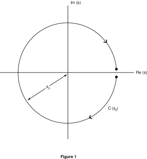
Figure 1: The contour $C\left(s_{0}\right)$.

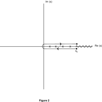
Figure 2: Distortion of the contour $C\left(s_{0}\right)$ appropriate for resonances and continuum contributions on the positive real-$s$ axis.

Remarkably, this insensitivity characterizes the second FESR $F_{1}(s_{0})$ as well [16]. To see this, we first substitute (5) into (4) when $k=1$:

$$F_{1}(s_{0}) = \sum_{r}\,\int_{0}^{s_{0}}\,S_{r}(s)\,s\,ds=\sum_{m_{r}^{2}<s_{0}}\,g_{r}\,\int_{0}^{\Gamma_{\rm{max}}}\,d\Gamma^{\prime}\frac{f(\Gamma^{\prime})}{2m_{r}\Gamma^{\prime}}\,\int_{(m_{r}^{2}-m_{r}\Gamma^{\prime})}^{(m_{r}^{2}+m_{r}\Gamma^{\prime})}\,ds\,s$$ (10)

$$= \sum_{m_{r}^{2}<s_{0}}\,g_{r}m_{r}^{2}\,\int_{0}^{\Gamma_{\rm{max}}}\,d\Gamma^{\prime}\,f(\Gamma^{\prime}).$$

We see, however, from explicit substitution of (7) into (8) that

$$\int_{0}^{\Gamma_{\rm{max}}}\,d\Gamma^{\prime}f(\Gamma^{\prime})=1,$$ (11)

in which case

$$F_{1}(s_{0})=\sum_{m_{r}^{2}<s_{0}}\,g_{r}m_{r}^{2}.$$ (12)

This result is independent of the width of the (symmetric) resonance peak $S_{r}(s)$, provided the entire resonance peak lies beneath the continuum-threshold $s_{0}$. Indeed, the result (12) also characterizes the narrow resonance approximation, as is evident upon substitution of (6) for $S_{r}(s)$ in the integral appearing within the first intermediate step of (10).

The results (9) and (12) are useful for constructing phenomenological constraints on the lightest $I=0$ scalar resonance. The two resonances with which we are specifically concerned are $f_{0}(980)$ and $f_{0}(400-1200)$; we shall henceforth denote the latter resonance as $\sigma$. Let us first suppose that only one of these two low-lying scalar resonances couples strongly to the $I=0$ $n\bar{n}$ scalar current (3). One might anticipate such behaviour if $f_{0}(980)$ were interpreted as a pure $s\bar{s}$ state, or a non-$q\bar{q}$ state, such as a $K\overline{K}$ molecule [17] or a four-quark $(qq\bar{q}\bar{q})$ exotic [4]. As long as $s_{0}$ is chosen low enough to exclude further $I=0$ $q\overline{q}$ scalar resonances, one finds from (9) and (12) that the lowest lying $q\bar{q}$ scalar resonance-mass is just

$$[m_{\sigma}^{2}]_{I}=F_{1}(s_{0})/F_{0}(s_{0}).$$ (13)

The “$I$” subscript implies only a single contributing $I=0$ scalar resonance to the FESR’s $F_{0}$ and $F_{1}$. Clearly, a $n\bar{n}$ interpretation of a light $\sigma$ is not viable in this scenario if $m_{\sigma}^{2}$, as obtained from (13) via QCD expressions for $F_{0,1}$, is larger than the experimental $\sim(700MeV)^{2}$ upper bound to an empirical light, broad $\sigma$-resonance in $\pi-\pi$ scattering [13, 14]. Indeed, if the lowest-lying $n\bar{n}$ resonance mass were found to be near $980{\rm\,MeV}$, a plausible interpretation would be to identify this resonance with $f_{0}(980)$, and to assume an exotic interpretation for the remaining $f_{0}(400-1200)$ state. Indeed, a recent OPAL study of $Z^{0}$ decays is found to support a $n\bar{n}$ interpretation of the $f_{0}(980)$ resonance state [18].

The requirement that $[F_{1}(s_{0})/F_{0}(s_{0})]^{\frac{1}{2}}$ be less than 980 MeV for a $n\bar{n}$ interpretation of a light $\sigma$ is found to hold even if we assume there to be two contributing $m\leq 1\,{\rm GeV}$ resonances to scalar current $I=0$ FESR’s. Suppose both $\sigma$ and $f_{0}(980)$ resonances contribute to the FESR’s $F_{0,1}$. Denoting the latter resonance by the subscript $f$, we see from (9) and (12) that

$$F_{0}=g_{\sigma}+g_{f},$$ (14)

$$F_{1}=g_{\sigma}(m_{\sigma}^{2})_{II}+g_{f}(m_{f}^{2}).$$ (15)

The subscript “$II$” denotes the $\sigma$-mass estimate assuming there to be two contributing resonances. One can solve (14,15) for $(m_{\sigma}^{2})_{II}$ to obtain

$$(m_{\sigma}^{2})_{II}=\left[\frac{F_{1}(s_{0})}{F_{0}(s_{0})}-m_{f}^{2}\right]\,\frac{F_{0}}{g_{\sigma}}+m_{f}^{2}.$$ (16)

Since $g_{\sigma}$, $F_{1}$, and $F_{0}$ are all positive, a consequence of the positivity of the measure $Im[\Pi(s)]ds$, it is evident from (16) that $(m_{\sigma}^{2})_{II}$ will be smaller than $m_{f}^{2}$ [presumably the square of the $f_{0}(980)$ mass] only if $F_{1}/F_{0}<m_{f}^{2}$. Thus, if $m_{f}$ is identified with the $f_{0}(980)$ mass, we see that $(F_{1}/F_{0})^{\frac{1}{2}}$ must be less than 980 MeV for the viability of a $n\bar{n}$ interpretation for the empirical observation of a light $\sigma$.

This result is simplified somewhat by considering the differences between $m_{\sigma}^{2}$ and $m_{f}^{2}$, where $m_{f}$ is now to be regarded as any contributing second resonance in the $I=0$ scalar channel:

$$\delta_{1}\equiv m_{f}^{2}-F_{1}/F_{0}=m_{f}^{2}-(m_{\sigma}^{2})_{I},$$ (17)

$$\delta_{2}\equiv m_{f}^{2}-(m_{\sigma}^{2})_{II}.$$ (18)

We see from (16) that

$$\delta_{2}=\frac{F_{0}}{g_{\sigma}}\,\delta_{1}.$$ (19)

The result (19) implies that if two resonances contribute to FESR’s $F_{0,1}$, it is possible to have a very light $\sigma$ coupled to a $n\bar{n}$ current via a scenario in which $\delta_{2}>\delta_{1}>0$ [i.e. $\left(m^{2}_{\sigma}\right)_{II}<\left(m^{2}_{\sigma}\right)_{I}<m_{f}^{2}$], provided the following two criteria are met:

1. $g_{\sigma}$ is small compared to $F_{0}$, and

2. $(F_{1}/F_{0})^{\frac{1}{2}}$ is smaller than $m_{f}$, the mass of the heavier resonance.

This latter criterion is necessary for the sign of $\delta_{1}$ to be positive, which is seen from (19) to be a necessary requirement for positivity of $\delta_{2}$. These criteria generalize to many resonances $m_{\sigma}<m_{1}<m_{2}<\ldots<m_{n}$ since

$$\frac{F_{1}}{F_{0}}=\frac{g_{\sigma}m_{\sigma}^{2}+g_{1}m_{1}^{2}+g_{2}m_{2}^{2}+\ldots+g_{n}m_{n}^{2}}{g_{\sigma}+g_{1}+g_{2}+\ldots+g_{n}}\leq m_{n}^{2}\quad.$$ (20)

Thus the second criterion above should be understood as a constraint on the heaviest contributing resonance consistent with the choice of continuum threshold $s_{0}$. Although the first criterion listed above is quite
reasonable, the latter criterion provides an important constraint on any attempt to model an empirical light broad $\sigma$ as a $q\overline{q}$ state.

3 Field-Theoretical Content of Scalar-Current FESR’s

QCD field-theoretical expressions for the sum rules $F_{0,1}(s_{0})$ are obtained from purely-perturbative, vacuum condensate, and instanton contributions to the scalar correlator $\Pi(s)$, as defined by (2). Both the purely-perturbative and the instanton contributions (nonperturbative contributions of finite correlation length) can be understood to have a branch singularity along the positive real-$s$ axis of Figure 1. By contrast, the QCD-vacuum condensate contributions (nonperturbative contributions of infinite correlation length) are characterized by poles at $s=0$, as obtained from the Wilson coefficients within the operator product expansion of the correlator. Consequently, purely-perturbative (pert), vacuum condensate (cond), and instanton (inst) contributions to the FESR’s $F_{k}(s_{0})$ can be obtained from (1) by distorting the contour $C(s_{0})$ as indicated in Figure 3:

$$F_{k}(s_{0})=\frac{1}{\pi}\,\int_{0}^{s_{0}}\left\{Im\left[\Pi(s,\mu^{2}=s_{0})\right]_{\rm{pert}}+Im[\Pi(s)]_{\rm{inst}}\right\}s^{k}ds-{\rm{Res}}_{s=0}\left\{s^{k}[\Pi(s)]_{\rm{cond}}\right\}.$$ (21)

The leading condensate contributions to the scalar correlation function can be extracted from refs. [20, 21, 22]:

$$[\Pi(s=-Q^{2})]_{\rm{cond}} = \frac{3m_{q}^{2}}{2Q^{2}}\langle m_{q}\overline{q}q\rangle+\frac{m_{q}^{2}}{16\pi Q^{2}}\langle\alpha_{s}G^{2}\rangle+\frac{m_{q}^{2}\pi}{Q^{4}}\langle{\cal O}_{6}\rangle+\frac{m_{q}^{3}}{2Q^{4}}\langle\overline{q}G\cdot\sigma q\rangle$$ (22)

$$+m_{q}^{4}\left[C_{1}\,\frac{\langle m_{q}\overline{q}q\rangle}{Q^{4}}+C_{2}\,\frac{\langle\alpha_{s}G^{2}\rangle}{Q^{4}}+C_{3}\,\frac{\langle\alpha_{s}(\overline{q}q)^{2}\rangle}{Q^{6}}+C_{4}\,\frac{\langle g_{s}G^{3}\rangle}{Q^{6}}\right].$$

The quantity $\langle{\cal O}_{6}\rangle$ denotes the following linear combination of dimension-six quark condensates:

$$\langle{\cal O}_{6}\rangle\equiv\alpha_{s}\left[\frac{1}{4}\langle\left(\bar{u}\sigma_{\mu\nu}\lambda^{a}u-\bar{d}\sigma_{\mu\nu}\lambda^{a}d\right)^{2}\rangle+\frac{1}{6}\langle\left(\bar{u}\gamma_{\mu}\lambda^{a}u+\bar{d}\gamma_{\mu}\lambda^{a}d\right)\sum_{u,d,s}\bar{q}\gamma^{\mu}\lambda^{a}q\rangle\right]\quad.$$ (23)

The vacuum saturation hypothesis [22] in the SU(2) limit $\langle\bar{u}u\rangle=\langle\bar{d}d\rangle\equiv\langle\bar{q}q\rangle$ provides a reference value for $\langle{\cal O}_{6}\rangle$

$$\langle{\cal O}_{6}\rangle=-f_{vs}\frac{88}{27}\alpha_{s}\langle(\bar{q}q)^{2}\rangle=-f_{vs}5.9\times 10^{-4}{\rm GeV}^{6}\quad,$$ (24)

where $f_{vs}=1$ for exact vacuum saturation. The quark condensate is determined by the GMOR (PCAC) relation [23], and the gluon condensate is given by [24]

$$\langle\alpha_{s}G^{2}\rangle=\left(0.045\pm 0.014\right)\,{\rm GeV^{4}}\quad.$$ (25)

The coefficients $C_{1}-C_{4}$ of $O(m_{q}^{4})$ terms are dimensionless and independent of $m_{q}$ after operator re-alignment [25] is imposed to circumvent mass singularities [$C_{2}$ and $C_{4}$ are seen [16] to still include factors of $\ln(Q^{2}/\mu^{2})$]. We see that all but the first three terms on the right hand side of (22) are chirally suppressed; the condensate $\langle m_{q}\overline{q}q\rangle=-f_{\pi}^{2}m_{\pi}^{2}/2$ [22, 23] is understood to have no explicit $m_{q}$-dependence ($f_{\pi}\equiv 93{\rm MeV}$). These three leading terms contribute to the residue portion of (21).

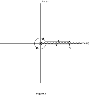
Figure 3: Distortion of the contour $C\left(s_{0}\right)$ appropriate for field-theoretical poles at $s=0$ and field-theoretical branch singularities along the entire positive real-$s$ axis.

The $n_{f}=3$ purely-perturbative QCD contribution to the imaginary part of the scalar correlator (2) has been calculated to four-loop order [26]:

$$\frac{1}{\pi}\,Im\left[\Pi(s,\mu^{2})\right]_{\rm{pert}} = \frac{3m_{q}^{2}s}{16\pi^{2}}\Biggl{[}1+\frac{\alpha_{s}}{\pi}\left(\frac{17}{3}-2\ln\left(\frac{s}{\mu^{2}}\right)\right)\Biggr{.}$$

$$\qquad+\left(\frac{\alpha_{s}}{\pi}\right)^{2}\left(31.8640-\frac{95}{3}\ln\left(\frac{s}{\mu^{2}}\right)+\frac{17}{4}\ln^{2}\left(\frac{s}{\mu^{2}}\right)\right)$$

$$\qquad+\Biggl{.}\left(\frac{\alpha_{s}}{\pi}\right)^{3}\left(89.1564-297.596\ln\left(\frac{s}{\mu^{2}}\right)+\frac{229}{2}\ln^{2}\left(\frac{s}{\mu^{2}}\right)-\frac{221}{24}\ln^{3}\left(\frac{s}{\mu^{2}}\right)\right)\Biggr{]}~{}.$$

The renormalization-group (RG) invariance of the correlator (2), as obtained from the RG invariant scalar current (3), allows RG improvement within the sum rule integrand (3) as follows ($\mu^{2}\equiv s_{0}$):

$$\alpha_{s}\longrightarrow\alpha_{s}(\sqrt{s_{0}}),$$ (27)

$$m_{q}\longrightarrow m_{q}(\sqrt{s_{0}}),$$ (28)

with the evolution of $\alpha_{s}(\mu)$ and $m_{q}(\mu)$ given by four-loop $\beta$ and $\gamma_{m}$ functions derived in refs. [27] and [28], respectively (see [29, 30] for explicit forms).

The imaginary part of the direct single-instanton contribution to the scalar correlator in the dilute instanton-liquid model is given by [10, 31]

$$\frac{1}{\pi}\,Im\left[\Pi(s)\right]_{\rm{inst}}=-\frac{3m_{q}^{2}s}{8\pi}\,J_{1}(\rho\sqrt{s})Y_{1}(\rho\sqrt{s}),$$ (29)

where $\rho$ is the (uniform) instanton size $\rho=1/(600\,{\rm MeV})$ appropriate for the instanton-liquid model [7]. We can now substitute (22–29) into (21) to obtain explicit expressions for the first two FESR’s:

$$\frac{F_{0}(s_{0})}{m_{q}^{2}(s_{0})} = \frac{3s_{0}^{2}}{32\pi^{2}}\left[1+\frac{20}{3\pi}\alpha_{s}(\sqrt{s_{0}})+\frac{49.8223}{\pi^{2}}\,\alpha_{s}^{2}(s_{0})+\frac{302.110}{\pi^{3}}\alpha_{s}^{3}(\sqrt{s_{0}})+{\cal{O}}(\alpha_{s}^{4})\right]$$ (30)

$$+\frac{3}{2}\langle m_{q}\overline{q}q\rangle+\frac{1}{16\pi}\langle\alpha_{s}G^{2}\rangle+{\cal{O}}(m_{q}^{2})-\frac{s_{0}^{2}}{8\pi}\left[J_{1}(\rho\sqrt{s_{0}})Y_{1}(\rho\sqrt{s_{0}})+J_{2}(\rho\sqrt{s_{0}})Y_{2}(\rho\sqrt{s_{0}})\right]\quad,$$

$$\frac{F_{1}(s_{0})}{m_{q}^{2}(s_{0})} = \frac{s_{0}^{3}}{16\pi^{2}}\left[1+\frac{19}{3\pi}\alpha_{s}(\sqrt{s_{0}})+\frac{43.3640}{\pi^{2}}\,\alpha_{s}^{2}(s_{0})+\frac{215.846}{\pi^{3}}\alpha_{s}^{3}(\sqrt{s_{0}})+{\cal{O}}(\alpha_{s}^{4})\right]$$ (31)

$$-\frac{3s_{0}^{3}}{160\pi}\left[5J_{1}(\rho\sqrt{s_{0}})Y_{1}(\rho\sqrt{s_{0}})+4J_{2}(\rho\sqrt{s_{0}})Y_{2}(\rho\sqrt{s_{0}})-J_{3}(\rho\sqrt{s_{0}})Y_{3}(\rho\sqrt{s_{0}})\right]$$

$$+\frac{88\pi}{27}f_{vs}\langle\alpha_{s}(\overline{q}q)^{2}\rangle+{\cal{O}}(m_{q})\quad.$$

We reiterate that these FESR’s are dual to phenomenological expressions that are independent of resonance-shape effects, as long as such resonance shapes are symmetric and entirely beneath the continuum threshold $s_{0}$. The instanton contributions to (30) and (31) are respectively obtained via the following indefinite integrals [32]:

$$\int z^{3}J_{1}(z)Y_{1}(z)dz=\frac{z^{4}}{6}\left[J_{1}(z)Y_{1}(z)+J_{2}(z)Y_{2}(z)\right]+{\rm constant},$$ (32)

$$\int z^{5}J_{1}(z)Y_{1}(z)dz=\frac{z^{6}}{8}\left[J_{1}(z)Y_{1}(z)+\frac{4}{5}J_{2}(z)Y_{2}(z)-\frac{1}{5}J_{3}(z)Y_{3}(z)\right]+{\rm constant}~{}~{}.$$ (33)

Equations (30) and (31) are sufficient to generate via (13) the estimate $(m_{\sigma})_{I}$ of the lowest-lying $I=0$ scalar meson, assuming this to be the only contributing resonance. In Figure 4, $(m_{\sigma})_{I}[\equiv(F_{1}/F_{0})^{\frac{1}{2}}]$ is displayed as a function of the continuum threshold parameter $s_{0}$ up to values comparable to $s_{0}=4\,{\rm GeV^{2}}$, using the central nonperturbative-parameter values defined above. The $s_{0}$-dependence of the coupling-constant $\alpha_{s}(\sqrt{s_{0}})$, which explicitly enters the right-hand sides of (30) and (31), is displayed in Figure 5, and is obtained (as described in ref. [33]) from the initial condition $\alpha_{s}(M_{Z})=0.119$ via the four-loop $\beta$-function with 4- and 5-flavour threshold discontinuities [34] at 1.3 GeV and 4.3 GeV, respectively. From Figure 4, we see that $(m_{\sigma})_{I}$ increases with $s_{0}$ and is never comparable to the empirical 400-700 MeV mass range anticipated from $\pi-\pi$ scattering phase shifts [13, 14]; even for the (unrealistically low) choice of $1\,{\rm GeV}^{2}$ for the continuum-threshold, the single-resonance fit for $m_{\sigma}$ is nearly $800\,{\rm MeV}$.

Figure 4: The quantity $\sqrt{F_{1}/F_{0}}$ is plotted as a function of $s_{0}$ using central values of the nonperturbative parameters as outlined in the text. The solid curve uses two-loop perturbative corrections, while the dotted curve uses four-loop corrections.

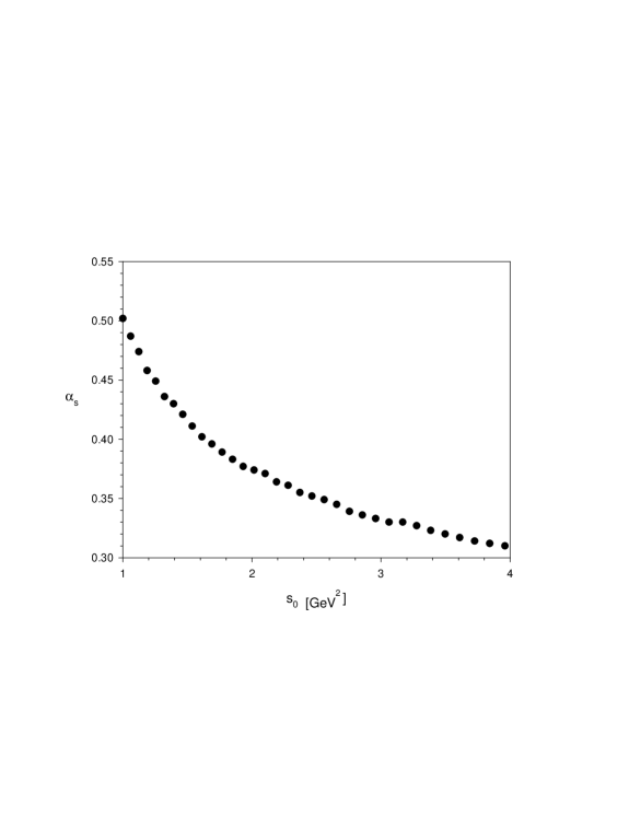
Figure 5: Evolution of the running coupling $\alpha_{s}$ versus the energy scale $s_{0}$ using $\alpha_{s}\left(M_{Z}\right)$ as an initial condition. Matching conditions imposed at the flavour thresholds are evident.

We see from Figure 4 that for values $1.0\,{\rm GeV}\leq\sqrt{s_{0}}\leq 1.3\,{\rm GeV}$ for which the $f_{0}(980)$ peak (but no subsequent resonance) is expected to contribute, the range of the single-resonance estimate of the lowest-lying $I=0$ $n\bar{n}$-resonance appears consistent with that resonance actually being $f_{0}(980)$. Such an interpretation of this state is consistent with a recent analysis of OPAL data [18], but would necessarily require a non-$n\bar{n}$ interpretation (or a mass near or above 1 GeV) for the $f_{0}(400-1200)$ state.

A drawback to the finite energy sum rule approach is its failure to suppress non-low-lying resonances, as is evident from (9) and (12). Recall that in the previous section, we examined the phenomenological consequences of having multiple resonances contribute to the FESR’s (30) and (31). A light resonance is found to be possible only if $(F_{1}/F_{0})^{\frac{1}{2}}$ is smaller than the mass of the heaviest contributing resonance. In a scenario in which there are now two contributing $n\bar{n}$ resonances, the $f_{0}(980)$ and a lighter (400-700 MeV) $\sigma$, we see from Figure 4 that the continuum threshold parameter $s_{0}$ is restricted to values below $1.6\,{\rm GeV^{2}}$, the value of $s_{0}$ at which $(F_{1}/F_{0})^{\frac{1}{2}}$ is equal to 980 MeV. In Section 5, we shall demonstrate via Holder-inequalities that this range of $s_{0}$ is excluded from sum-rule parameter space – consequently, we can rule out the scenario in which $f_{0}(980)$ and an even lighter $\sigma$ both contribute (as $n\bar{n}$-resonances) to the first two FESR’s. We cannot, however, exclude the possibility of such a light $\sigma$ hiding under the large contribution of $f_{0}(1370)$, assuming an $n\bar{n}$ interpretation for this state [35], as the value of $(F_{1}/F_{0})^{\frac{1}{2}}$ is still below $1370\,{\rm MeV}$ for values of $s_{0}$ as large as $3.5\,{\rm GeV^{2}}$. Indeed, similar behaviour characterizes the pseudoscalar channel, where sum rule contributions from the first pion excitation [$\Pi(1300)$] dominate those of the lowest-lying pseudoscalar resonance, the pion itself [36].

Summarizing, we find that the first two finite-energy sum rules have the advantage of being insensitive to widths of (symmetric) subcontinuum resonance peaks. They have the disadvantage of failing to suppress contributions from non-lowest-lying subcontinuum resonances. For the suppression of such resonances within a sum rule context, we necessarily must employ width-sensitive Laplace sum rules, as previously considered in ref. [5]. Such sum rules $R_{k}(\tau,s_{0})$ are defined similarly to the FESR’s (1) except for the occurrence of an exponential damping factor $e^{-s\tau}$ in the sum-rule integrand:

$$R_{k}(\tau,s_{0})=\frac{1}{2\pi i}\,\int_{C(s_{0})}\,\Pi(s)s^{k}e^{-s\tau}ds.$$ (34)

If we substitute the phenomenological resonance content of $Im\Pi$, as given in (5), and utilize the narrow resonance approximation (6), we find there to be a progressive exponential suppression of heavy resonances within such sum rules [22], in contrast to the resonance content of corresponding FESR’s given by (9) and (12):

$$R_{0}(\tau,s_{0})=\sum_{m_{r}^{2}<s_{0}}\,g_{r}e^{-m_{r}^{2}\tau},$$ (35)

$$R_{1}(\tau,s_{0})=\sum_{m_{r}^{2}<s_{0}}\,g_{r}m_{r}^{2}e^{-m_{r}^{2}\tau}.$$ (36)

The contribution of the lowest-lying resonance $(\ell)$ is pronounced provided the Borel-parameter $\tau$ is chosen so as to be less than the reciprocal of the square of the mass of the lightest resonance $(m_{\ell}^{2}\tau<1)$, but greater than the reciprocal of the square of the mass of any subsequent $(h)$ resonance $(m_{h}^{2}\tau>1)$. In the section which follows, we shall examine in detail the field theoretical content of the leading Laplace sum rule in the scalar channel, particularly its instanton content as extracted from (34).

4 Field-Theoretical Content of the Laplace Sum-Rule

The leading Laplace sum-rule $R_{0}(\tau,s_{0})$ may be obtained from (34) by distorting the contour $C(s_{0})$ as indicated in Figure 3, a procedure identical to that by which the FESR’s (21) are calculated from (1):

$$R_{0}(\tau,s_{0})=\frac{1}{\pi}\int\limits_{0}^{s_{0}}\left\{Im\left[\Pi(s)\right]_{pert}+Im\left[\Pi(s)\right]_{inst}\right\}e^{-s\tau}ds-{\rm Res}_{s=0}\left\{e^{-s\tau}\left[\Pi(s)\right]_{cond}\right\}\quad.$$ (37)

It is customary, however, to express this sum-rule as the difference between its $s_{0}\rightarrow\infty$ limit and a continuum-contribution $c_{0}(\tau,s_{0})$, which is seen from (37) to be the following:

$$R_{0}(\tau,s_{0})=R_{0}(\tau,\infty)-c_{0}(\tau,s_{0})\quad,$$ (38)

$$R_{0}(\tau,s_{0})=\frac{1}{\pi}\int\limits_{0}^{s_{0}}Im\Pi^{res}(s)e^{-s\tau}\,ds\quad,$$ (39)

$$c_{0}(\tau,s_{0})=\frac{1}{\pi}\int\limits_{s_{0}}^{\infty}\left\{Im\left[\Pi(s)\right]_{pert}+Im\left[\Pi(s)\right]_{inst}\right\}e^{-s\tau}ds=c_{0}^{pert}(\tau,s_{0})+c_{0}^{inst}(\tau,s_{0})\quad.$$ (40)

We see from substitution of (22), (3), and (29) into the $s_{0}\rightarrow\infty$ limit of (37) that, for $I=\{0,1\}$ [21, 22, 37],

$${R}_{0}(\tau,\infty) = \frac{3m_{q}^{2}}{16\pi^{2}\tau^{2}}\left(1+4.821098\frac{\alpha_{s}}{\pi}+{\cal O}\left[\alpha_{s}^{2}\right]\right)+m_{q}^{2}\left(\frac{3}{2}\langle m_{q}\bar{q}q\rangle+\frac{1}{16\pi}\langle\alpha_{s}G^{2}\rangle+\pi\langle{\cal O}_{6}\rangle\tau\right)$$ (41)

$$\qquad+\left(-1\right)^{I}m_{q}^{2}{3\rho^{2}\over{16\pi^{2}\tau^{3}}}e^{-\frac{\rho^{2}}{2\tau}}\left[K_{0}\left(\frac{\rho^{2}}{2\tau}\right)+K_{1}\left(\frac{\rho^{2}}{2\tau}\right)\right]\quad.$$

We have included within (41) only the two-loop perturbative contribution, as condensate contributions are known to only one-loop order. Sum-rule stability under higher-loop perturbative expressions will be discussed in section 6.3. The sum-rules $R_{k}(\tau,\infty)$ are known [38] to satisfy RG equations with respect to the mass scale $\mu=1/\sqrt{\tau}$, thereby justifying the following two-loop order RG improvements:

$$\frac{\alpha_{s}}{\pi}\rightarrow\frac{\alpha_{s}(\mu)}{\pi}=\frac{1}{\beta_{0}L}-\frac{\beta_{1}\log L}{\beta_{0}\left(\beta_{0}L\right)^{2}}\quad,$$ (42)

$$L=\log\left(\frac{\mu^{2}}{\Lambda^{2}}\right)\quad,\quad\beta_{0}=\frac{9}{4}\quad,\quad\beta_{1}=4\quad;$$ (43)

$$m_{q}\rightarrow m_{q}(\mu)\equiv\hat{m}_{q}G(\mu)\quad,$$ (44)

$$G(\mu)=\frac{1}{\left(\frac{1}{2}L\right)^{\frac{4}{9}}}\left(1+\frac{290}{729}\frac{1}{L}-\frac{256}{729}\frac{\log{L}}{L}\right)\quad.$$ (45)

We use $\Lambda_{\overline{MS}}\approx 300\,{\rm MeV}$ for three active flavours, consistent with current estimates of $\alpha_{s}(M_{\tau})$ [1, 39] and matching conditions through the charm threshold [34].

The above formulation differs from past treatments (even those in which the instanton contribution to $R_{0}$ is explicit [5]) in which only purely-perturbative effects contribute to the continuum (40). We see from substitution of (29) into (40) that methodological consistency requires an explicit instanton contribution to the continuum,

$$c_{0}^{inst}\left(\tau,s_{0}\right)=\left(-1\right)^{I+1}\frac{3m_{q}^{2}}{8\pi}\int\limits_{s_{0}}^{\infty}sJ_{1}\left(\rho\sqrt{s}\right)Y_{1}\left(\rho\sqrt{s}\right)e^{-s\tau}\,ds\quad,$$ (46)

in addition to the known perturbative contribution arising from (3):

$$c_{0}^{pert}\left(\tau,s_{0}\right)=\frac{3m_{q}^{2}}{16\pi^{2}}\left[\left(1+\frac{17}{3}\frac{\alpha_{s}}{\pi}\right)f_{0}\left(\tau,s_{0}\right)-2\frac{\alpha_{s}}{\pi}f_{1}\left(\tau,s_{0}\right)\right]\quad,$$ (47)

$$f_{0}\left(\tau,s_{0}\right)=\frac{1}{\tau^{2}}\left(1+s_{0}\tau\right)e^{-s_{0}\tau}\quad,$$ (48)

$$f_{1}\left(\tau,s_{0}\right)=\frac{1}{\tau^{2}}\left[\left(1+s_{0}\tau\right)e^{-s_{0}\tau}\log\left(s_{0}\tau\right)+e^{-s_{0}\tau}+E_{1}\left(s_{0}\tau\right)\right]\quad.$$ (49)

In the above equations $\gamma_{E}$ is Euler’s constant and $E_{1}(x)$ is the exponential integral.

We reiterate that the instanton continuum contribution has been ignored in previous applications of instanton effects in sum-rules. To determine the numerical significance of this contribution, we compare the total instanton contributions to the sum-rule (37) before and after inclusion of the instanton continuum. As shown in Figure 6, inclusion of the continuum enhances the total instanton contributions. Since the instanton effects without the continuum are responsible for the $\sim 500\,{\rm MeV}$ splitting between the lowest-lying $I=0$ and $I=1$ states found in [5], enhancement of the instanton effects suggests that an even larger isospin splitting could occur by including the instanton contribution to the continuum (40). Furthermore, it is interesting to note that integration of (46) with the instanton density $d(\rho)$ will be well behaved at small $\rho$ because $J_{1}\left(\rho\sqrt{t}\right)$ goes to zero for small $\rho$. This behaviour should be contrasted with that of [10, 22]

$$\Pi^{inst}(s=-Q^{2})=\left(-1\right)^{I}\frac{3}{4\pi^{2}}m_{q}^{2}Q^{2}\left[K_{-1}\left(\rho\sqrt{Q^{2}}\right)\right]^{2}\quad,$$ (50)

which has an infrared divergence when integrated over $\rho$.

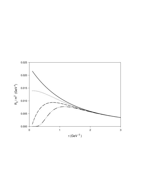
Figure 6: Comparison of the instanton contributions to the Laplace sum-rule with inclusion of the instanton continuum (upper three curves), and omission of the instanton continuum (lowest dashed-dotted curve). The $s_{0}$ values used for evaluation of the instanton continuum are: $s_{0}=2.5\,{\rm GeV^{2}}$ (solid curve), $s_{0}=3.0\,{\rm GeV^{2}}$ (dotted curve), and $s_{0}=3.5\,{\rm GeV^{2}}$ (dashed curve).

5 Hölder Inequality Constraints on the Laplace Scalar Sum-Rules

In the phenomenological analysis of QCD sum-rules, the $\tau$-dependence of $R_{0}(\tau,s_{0})$, as given by (38), (41), (46) and (47), is used to extract phenomenological resonance parameters $g_{r}$ and $m_{r}^{2}$ within (35). Such an analysis, however, is predicated on having some knowledge of the $\tau$ range for which comparison of the theoretical content of $R_{0}(\tau,s_{0})$ to (35) is a valid exercise [22, 40]. This question can be addressed by Hölder inequalities, which must be upheld for Laplace sum-rules to retain consistency with the physical positivity of the resonance content (5) of ${\rm Im}\Pi^{res}(s)$ [9]:

$$\frac{{R}_{0}[\omega\tau+(1-\omega)\delta\tau,s_{0}]}{\left({R}_{0}[\tau,s_{0}]\right)^{\omega}\left({R}_{0}[\tau+\delta\tau,s_{0}]\right)^{1-\omega}}\leq 1\quad,\quad\forall~{}0\leq\omega\leq 1\quad.$$ (51)

If $\delta\tau$ is reasonably small ($\sim 0.1\,{\rm GeV}^{-2}$ [9]), these inequalities are themselves insensitive to the choice of $\delta\tau$, in which case the requirement (51) can be used to determine a range for the Borel parameter $\tau$ itself, given a chosen value for the continuum threshold $s_{0}$. Such Hölder inequalities have in the past been used to place bounds on the light-quark masses and on the pion polarizability [41], as well as the parameter space of QCD sum-rule analyses.

The inequality (51) can be demonstrated to support the presence of an instanton contribution to the continuum $c_{0}(\tau,s_{0})$, as this contribution alters the region in $(\tau,s_{0})$ parameter space for which (51) is upheld. Figure 7 shows the region of this parameter space satisfying the inequality (51) when instantons contribute to $c_{0}(\tau,s_{0})$ in the isoscalar case. The shape of the region is quite similar to that which characterizes other sum rules [9]. Omission of this instanton contribution from the continuum leads to the less restrictive parameter space shown in Figure 8, which seems to imply the validity of local duality at very low values of $s_{0}$ that are generally Hölder-inequality excluded.

Figure 7: Data points indicate values of $\tau$ and $s_{0}$ for which the $I=0$ sum-rule with inclusion of the instanton continuum satisfies the Hölder inequality. The scales are in GeV units.

Figure 8: Data points indicate values of $\tau$ and $s_{0}$ for which the $I=0$ sum-rule with omission of the instanton continuum satisfies the Hölder inequality. The scales are in GeV units.

Figures 9 and 10 show the effect of the instanton continuum on the inequality analysis for the isovector channel. If the instanton contribution is removed (Figure 10), the parameter space for which (51) is upheld is restricted to substantially larger values of $s_{0}$ than is the case when the instanton contribution to the continuum is retained (Figure 9). Inclusion of the instanton continuum again leads to behaviour characteristic of other sum-rules [9]. Thus we see that if the instanton contribution to the continuum is removed, the $(\tau,s_{0})$ parameter space allowed by (51) increases in the isoscalar channel and decreases in the isovector channel, thereby enhancing unrealistically the discrepancy between the minimum value of the continuum threshold characterizing these two channels.

Figure 9: Data points indicate values of $\tau$ and $s_{0}$ for which the $I=1$ sum-rule with inclusion of the instanton continuum satisfies the Hölder inequality. The scales are in GeV units.

Figure 10: Data points indicate values of $\tau$ and $s_{0}$ for which the $I=1$ sum-rule with omission of the instanton continuum satisfies the Hölder inequality. The scales are in GeV units.

Thus the parameter space consistent with (51) appears to favour instanton contributions to the continuum, consistent with the methodology of the previous section. The allowed regions of the parameter space for the isoscalar (Figure 7) and isovector (Figure 9) channels are conservatively given by

$$0.3\,{\rm GeV}^{-2}\leq\tau\leq 1.7\,{\rm GeV}^{-2}~{},~{}s_{0}>3\,{\rm GeV}^{2}\quad(I=0),$$ (52)

$$0.3\,{\rm GeV}^{-2}\leq\tau\leq 1.1\,{\rm GeV}^{-2}~{},~{}s_{0}>4\,{\rm GeV}^{2}\quad(I=1).$$ (53)

It should be noted here that the absolute lower bound on $s_{0}$ in (52) excludes the $s_{0}\leq 1.6\,{\rm GeV^{2}}$ range, as determined in Section 3, for which FESR’s allow a light $n\bar{n}$ $\sigma$ resonance to be masked by the heavier $f_{0}(980)$. However, the possibility that such FESR masking of a light $n\bar{n}$ $\sigma$ occurs via the heavier $f_{0}(1370)$, as discussed at the end of Section 3, is still marginally allowed by the Hölder inequality (51). Recall from Section 3 that for such a masking to occur, the necessary condition that $\left(F_{1}/F_{0}\right)^{1/2}\leq 1.37\,{\rm GeV}$ is upheld provided $s_{0}<3.5\,{\rm GeV^{2}}$, an upper bound that is seen to be near the very bottom of the permitted parameter space in Figure 7. Consequently, such a scenario cannot at this juncture be ruled out, and requires exploration by Laplace sum rules over Hölder-inequality allowed parameter space.

Finally, we note that the upper bound on the $\tau$-range in (52) insures that exponential factors in (35) will not suppress any isoscalar resonance lighter than $800\,{\rm MeV}$, ensuring that the Laplace sum-rule remains an appropriate tool for extracting a 400–700 MeV $\sigma$ resonance. Moreover, the upper bound in (53) similarly ensures that an isovector resonance lighter than $1\,{\rm GeV}$ will also not be subject to exponential suppression, in which case the sum-rule in the isovector channel should be sensitive to $a_{0}(980)$ contributions. We shall see in the section that follows that neither of these candidates for the lowest-lying $n\bar{n}$ resonance in their respective channels are evident from the Laplace sum-rule $R_{0}(\tau,s_{0})$, suggesting that both the $\sigma(500)$ [if such a state exists at all] and the $a_{0}(980)$ should be interpreted either as non $q\bar{q}$ resonance states or as $q\bar{q}$ states with negligible $n\bar{n}$ content.

6 Phenomenological Analysis of Laplace Sum-Rules

6.1 Single-Resonance Analysis

In Section 4 it was also shown that we can anticipate enhanced splitting between isopartner states resulting from an instanton contribution to the continuum, suggesting a need to revisit the sum-rule analysis of [5] for the $n\bar{n}$ component of the lowest-lying $I=\{0,1\}$ quark ($q\bar{q}$) scalar mesons. The sum-rule predictions of the properties of these lowest-lying $I=\{0,1\}$ $n\bar{n}$ scalar resonances can now be studied through (39), which is assumed for now to be dominated by the lowest-lying resonance (as discussed at the end of Section 3). Since the widths of such resonances may be substantial, it is necessary to extend the narrow width approximation traditionally used in sum-rules. A flexible and numerically simple technique is to build up the resonance shape (7) within $Im\Pi(s)$ [eq. (5)] by utilizing $n$ unit-area square pulses [5, 42], thereby replacing (7) with the following expression:

$$S_{r}^{(n)}(s) = \frac{2}{n\pi}\sum_{j=1}^{n}\sqrt{\frac{n-j+f}{j-f}}P_{M_{r}}\left[s,\sqrt{\frac{n-j+f}{j-f}}\;\Gamma_{r}\right]\quad,$$ (54)

$$P_{M}\left[s,\Gamma\right] \equiv \frac{1}{2M\Gamma}\left[\Theta(s-M^{2}+M\Gamma)-\Theta(s-M^{2}-M\Gamma)\right]\quad.$$ (55)

A single square pulse models a broad nearly structureless contribution (such as a broad light $\sigma$) to ${\rm Im}\Pi(s)$, while a Breit-Wigner resonance of a particle of mass $M$ and width $\Gamma$ can be expressed as a sum of a number of square pulses. The quantity $f$ can be fixed by normalizing the area of the n-pulse approximation to unity.

We begin the phenomenological analysis with the $n=4$ pulse approximation (54) to the resonance shape so that the right-hand side of (39) becomes

$$\frac{1}{\pi}{\rm Im}\Pi^{res}=g_{r}S_{r}^{(4)}(s)\quad,$$ (56)

$${R}_{0}(\tau,s_{0})=g_{r}e^{-M^{2}\tau}W_{4}(M,\Gamma,\tau)\quad,$$ (57)

$$W_{4}(M,\Gamma,\tau)=\frac{2}{4\pi}\sum_{j=1}^{4}\frac{1}{M\Gamma\tau}\sinh\left[M\sqrt{\frac{4-j+0.7}{j-0.7}}\,\Gamma\tau\right]\quad,$$ (58)

where $\sqrt{g_{r}}$ is proportional to the strength with which the scalar $n\bar{n}$ current couples the vacuum to the resonance. As noted earlier, we are ignoring all but the lowest-lying resonance contribution to (5) in part because of the anticipated exponential suppression of subsequent resonances [e.g. (35) ]. The free parameters in the relation (57), the resonance-related quantities $g_{r}$, $M$, $\Gamma$ and the continuum-threshold $s_{0}$, can be extracted from a fit to the $\tau$ dependence of the theoretical expression ${R}_{0}(\tau,s_{0})$. This is done by minimizing the $\chi^{2}$ defined by

$$\chi^{2}=\frac{1}{N}\sum_{j=1}^{N}\frac{\left[{R}_{0}\left(\tau_{j},s_{0}\right)-g_{r}e^{-M^{2}\tau_{j}}W_{4}(M,\Gamma,\tau_{j})\right]^{2}}{\epsilon(\tau_{j})^{2}}\quad,$$ (59)

where the sum is over evenly spaced, discrete $\tau$ points in the ranges (52,53) consistent with the Hölder inequality. The weighting factor $\epsilon$ used for the evaluation of (59) is $\epsilon(\tau)=0.2R_{0}(\tau,s_{0})$. This 20% uncertainty has the desired property of being dominated by the continuum at low $\tau$ and power-law corrections at large $\tau$. Other choices of the $0.2$ prefactor in $\epsilon$ would simply rescale the $\chi^{2}$, so its choice has no effect on the values of the $\chi^{2}$-minimizing parameters.

In the $\chi^{2}$ minimization, the RG-invariant quark mass parameter $\hat{m}_{q}$ (44) is now absorbed into the quantity $a=g_{r}/\hat{m}_{q}^{2}$. The best-fit parameters for the $I=\{0,1\}$ channels are shown in Table 1. Since the resonance widths are sufficiently small to permit a series expansion of the $n$-pulse approximation (i.e. $M\Gamma\tau$ is small), it is impossible for $\chi^{2}$-minimization to distinguish between the $n=4$ and $n=1$ approximations; each has the same $\tau$ dependence to second order in their series expansions. Thus there is no possibility of distinguishing between a structureless resonance shape represented by $n=1$ and a Breit-Wigner-like form represented by $n=4$. We will continue to use the four-pulse approximation since it will lead to values for $\Gamma$ that correspond to a Breit-Wigner width [42].

$I$	$M~{}(GeV)$	$s_{0}~{}(GeV^{2})$	$a~{}(GeV^{4})$	$\Gamma~{}(GeV)$
0	$0.97$	$3.6$	$0.073$	$0.24$
1	$1.50$	$4.5$	$0.16$	$0.20$

Table 1: Values for the resonance parameters and continuum threshold for the $I=\{0,1\}$ channels which lead to a minimum $\chi^{2}$.

In principle the $2\pi$ continuum should also be included in the phenomenological model. However, the values for $a$ in Table 1 lead to a resonance contribution which is much larger than the $2\pi$ continuum [43]:

$$\frac{1}{\hat{m}_{q}^{2}}\frac{1}{\pi}{\rm Im}\,\Pi^{2\pi}(t)=\frac{3}{16\pi^{2}}\left|F(t)\right|^{2}\theta\left(t-4m_{\pi}^{2}\right)\quad,\quad F(t)\approx m_{\pi}^{2}\left(1+\frac{1}{6}\langle r_{\pi}^{2}\rangle t\right)\quad.$$ (60)

To determine the uncertainties associated with the best-fit parameters of Table 1 we perform a Monte-Carlo simulation which includes the parameter ranges $1\leq f_{vs}\leq 2$ and a 15% variation in the instanton size $\rho$. Using the technique of [36], we also simulate continuum and OPE-truncation uncertainties from the empirical functions

$$\epsilon(\tau)=a_{1}\exp{\left[-1.1\tau^{0.73}\right]}\quad,\quad I=0\quad;\quad\epsilon(\tau)=a_{2}\tau\exp{\left[-5.7\tau^{0.53}\right]}\quad,\quad I=1\quad,$$ (61)

where $|a_{1}|\leq 0.17$ and $|a_{2}|\leq 1.15$ in the Monte-Carlo simulation.

The Monte-Carlo simulation leads to the 90% confidence level results for the best-fit parameters shown in Table 2. These results indicate an absence of both the isovector $a_{0}(980)$ resonance as well as a very broad $400$–$700\,{\rm MeV}$ isoscalar $\sigma$ state, suggesting that neither of these states are primarily $n\bar{n}$ mesons; both appear to be decoupled from sum-rules based upon the $n\bar{n}$ scalar current (3). As mentioned earlier, decreasing the number of pulses (to simulate a structureless resonance) does not alter the $\chi^{2}$, and only leads to a rescaling of $\Gamma$. The large uncertainty in the width $\Gamma$ indicates the difficulty associated with predicting widths from QCD sum-rules, a problem which merits future consideration. An alternative choice for the resonance model will be considered in Section 6.5.

$I$	$M~{}(GeV)$	$s_{0}~{}(GeV^{2})$	$a~{}(GeV^{4})$	$\Gamma~{}(GeV)$
0	$1.00\pm 0.09$	$3.7\pm 0.4$	$0.08\pm 0.02$	$0.19\pm 0.14$
1	$1.55\pm 0.11$	$5.0\pm 0.7$	$0.17\pm 0.04$	$0.22\pm 0.11$

Table 2: Results of the Monte-Carlo simulation of 90% confidence-level uncertainties for the resonance parameters and continuum threshold for the $I=\{0,1\}$ channels.

6.2 Multi-Resonance Scenarios

A simple extension of the single resonance model (57) is a model with the incoherent sum of two resonances. The best fits in such a model lead to results which either are degenerate to the single resonance values of Table 1, or which do not significantly reduce the $\chi^{2}$ compared with the single resonance model. The latter case indicates that the second resonance is weak enough to be absorbed into the continuum, implying a decoupling from the $n\bar{n}$ scalar current.

To study quantitatively this apparent decoupling of a light $\sigma$ and the $a_{0}(980)$ from the quark ($n\bar{n}$) scalar current, we employ a two-resonance version of (57) in which the masses and widths of the resonances are used as input parameters. The two-resonance model couplings (i.e. the parameter $a=g_{r}/\hat{m}_{q}^{2}$ for each resonance) and continuum threshold $s_{0}$ which minimize $\chi^{2}$ are explicitly calculated.

As input we utilize the PDG values [1] for the $f_{0}(980)$, $a_{0}(980)$, $a_{0}(1450)$, as well as a $\sigma$ with $M=500\,{\rm MeV}$ and $\Gamma=500\,{\rm MeV}$. Since the $f_{0}(980)$ and $a_{0}(1450)$ PDG values are consistent with the fits of Table 2, we anticipate that if $a_{0}(980)$ and $\sigma$ are truly decoupled from the $n\bar{n}$ quark scalar currents, then the $\chi^{2}$-minimizing values of the $a_{0}(1450)$ coupling, $f_{0}(980)$ coupling, and $s_{0}$ should reproduce those given in Table 1. Although the observed hadronic states could in general contain a mixture of $n\bar{n}$, $s\bar{s}$, and possibly meson-meson or four-quark components, any state with a non-zero $n\bar{n}$ component will couple optimally to the scalar current (3) [the more exotic components may couple to (3) as well, but to a lesser degree]. Consequently, a large suppression of a resonance within the context of an $n\bar{n}$-current sum-rule analysis is indicative of a reduction of that same resonance’s explicit $n\bar{n}$ content.

Table 3 displays the results of this analysis. The fitted values of the $a_{0}(1450)$ coupling, the $f_{0}(980)$ coupling, and $s_{0}$ are virtually identical to those of Table 1. Furthermore, Table 3 shows that the $\sigma$ and $a_{0}(980)$ have couplings to the $n\bar{n}$ scalar current which are significantly suppressed compared with those of the $f_{0}(980)$ and $a_{0}(1450)$.

Since the FESR results of Section 3 suggest the possibility of a light $\sigma$ hiding beneath the $f_{0}(1370)$, we extend the isoscalar results of Table 3 by including the $f_{0}(1370)$. The results of this extension shown in Tables 4 and 5 indicate a suppression of the $\sigma$ and $f_{0}(1370)$ couplings to the $n\bar{n}$ current (3) compared with that of the $f_{0}(980)$.

$I$	$s_{0}~{}(GeV^{2})$	State	$M~{}(GeV)$	$\Gamma~{}(GeV)$	$a~{}(GeV^{4})$
1	$4.4$	$a_{0}(980)$	$0.98$	$0.1$	$0.0075$
1	$4.4$	$a_{0}(1450)$	$1.45$	$0.2$	$0.16$
0	$3.7$	$\sigma$	$0.5$	$0.5$	$0.0051$
0	$3.7$	$f_{0}(980)$	$0.98$	$0.1$	$0.068$

Table 3: Best fit values for the couplings and $s_{0}$ in a multi-resonance scenario. The masses and widths were used as input values.

$s_{0}~{}(GeV^{2})$	State	$M~{}(GeV)$	$\Gamma~{}(GeV)$	$a~{}(GeV^{4})$
$3.8$	$\sigma$	$0.5$	$0.5$	$0.0057$
$3.8$	$f_{0}(980)$	$0.98$	$0.1$	$0.065$
$3.8$	$f_{0}(1370)$	$1.37$	$0.2$	$0.0055$

Table 4: Best fit values for the couplings and $s_{0}$ in a multi-resonance scenario for the isoscalar channel with the PDG [1] lower bound on the $f_{0}(1370)$ width.

$s_{0}~{}(GeV^{2})$	State	$M~{}(GeV)$	$\Gamma~{}(GeV)$	$a~{}(GeV^{4})$
$3.7$	$\sigma$	$0.5$	$0.5$	$0.0051$
$3.7$	$f_{0}(980)$	$0.98$	$0.1$	$0.068$
$3.7$	$f_{0}(1370)$	$1.37$	$0.5$	$0.00098$

Table 5: Best fit values for the couplings and $s_{0}$ in a multi-resonance scenario for the isoscalar channel with the PDG [1] upper bound on the $f_{0}(1370)$ width.

The above results can be interpreted by recalling that the parameter $a$ is related to the strength of the coupling of the hadronic state $|H\rangle$ to the vacuum via the $n\bar{n}$ current.

$$a\sim\left|\langle O|n\bar{n}|H\rangle\right|^{2}$$ (62)

Hence it is clear from Tables 3–5 that the $\sigma$ and $a_{0}(980)$ have substantially reduced coupling to the $n\bar{n}$ current than the dominant states $f_{0}(980)$ and $a_{0}(1450)$, suggesting a non-$n\bar{n}$ interpretation of the $\sigma$ and $a_{0}(980)$. For example, the coupling of a meson-meson state to the vacuum through a $q\bar{q}$ current is likely to be suppressed compared to that of a $q\bar{q}$ state. Certainly at the QCD level, the mixing of local $q\bar{q}$ and $qq\bar{q}\bar{q}$ currents will be chirally suppressed by quark mass factors, which suggests a theoretical basis for this decoupling.

The relative strength of the couplings obtained in Tables 3–5 can be used as an estimate of the $n\bar{n}$ content of the known hadronic states. If the dominant states with the largest coupling are nearly pure $n\bar{n}$, and if there is minimal interference in the mixing between the $n\bar{n}$ and other components (such as meson-meson or four-quark components) of the non-dominant states, then Tables 3–5 indicate that the $a_{0}(980)$ has a relative $n\bar{n}$-content given approximately by $\sqrt{0.0075/0.16}\approx 20\%$, and that the $n\bar{n}$ content of the $\sigma$ is approximately 25–30%. If the dominant states are themselves admixtures, then the $n\bar{n}$-content of the $a_{0}(980)$ and $\sigma$ is correspondingly reduced.

Another important consequence of this analysis is the clear distinction that emerges between $f_{0}(980)$ and $a_{0}(980)$, since the former appears as the dominant state, and the latter appears to be coupled only weakly in comparison with the dominant isovector-channel state $a_{0}(1450)$. Such a distinction is important, since both $980\,{\rm MeV}$ states are close to the $K\bar{K}$ kinematic threshold. Consequently, both states might be expected to be dominated by comparably large $K\bar{K}$ components, in which case both states would exhibit comparably suppressed couplings to $n\bar{n}$-current scalar-channel sum rules. The disparity we find, however, is indicative of substantial $n\bar{n}$ content in $f_{0}(980)$, a result with some experimental support [18].

6.3 Higher-Loop Perturbative Effects

The effect of higher order perturbative contributions on the resonance parameters can now be studied. The perturbative part of the correlation function is known to four-loop order [26], modifying (37) as follows:

$${R}_{0}(\tau,\infty) = \frac{3m_{q}^{2}}{16\pi^{2}\tau^{2}}\left(1+4.821098\frac{\alpha_{s}}{\pi}+21.97646\left(\frac{\alpha_{s}}{\pi}\right)^{2}+53.14179\left(\frac{\alpha_{s}}{\pi}\right)^{3}\right)$$

$$+ m_{q}^{2}\left(\frac{3}{2}\langle m_{q}\bar{q}q\rangle+\frac{1}{16\pi}\langle\alpha_{s}G^{2}\rangle+\pi\langle{\cal O}_{6}\rangle\tau\right)+\left(-1\right)^{I}m_{q}^{2}{3\rho^{2}\over{16\pi^{2}\tau^{3}}}e^{-\frac{\rho^{2}}{2\tau}}\left[K_{0}\left(\frac{\rho^{2}}{2\tau}\right)+K_{1}\left(\frac{\rho^{2}}{2\tau}\right)\right].$$

Similarly, the continuum contributions (47) to four-loop order become

$$c_{0}^{pert}\left(\tau,s_{0}\right)=\frac{1}{\pi}\int\limits_{s_{0}}^{\infty}Im\Pi^{pert}(s)e^{-s\tau}\,ds\quad,$$ (64)

$$c_{0}^{{pert}}\left(\tau,s_{0}\right)=\frac{3m_{q}^{2}}{16\pi^{2}}\left[A_{0}f_{0}\left(\tau,s_{0}\right)+A_{1}f_{1}\left(\tau,s_{0}\right)+A_{2}f_{2}\left(\tau,s_{0}\right)+A_{3}f_{3}\left(\tau,s_{0}\right)\right]\quad,$$ (65)

$$A_{0}=1+\frac{17}{3}\frac{\alpha_{s}}{\pi}+31.8640\left(\frac{\alpha_{s}}{\pi}\right)^{2}+89.1564\left(\frac{\alpha_{s}}{\pi}\right)^{3}~{},~{}A_{1}=-2\frac{\alpha_{s}}{\pi}-\frac{95}{3}\left(\frac{\alpha_{s}}{\pi}\right)^{2}-297.596\left(\frac{\alpha_{s}}{\pi}\right)^{3}~{},$$ (66)

$$A_{2}=\frac{17}{4}\left(\frac{\alpha_{s}}{\pi}\right)^{2}+\frac{229}{2}\left(\frac{\alpha_{s}}{\pi}\right)^{3}\quad,\quad A_{3}=-\frac{221}{24}\left(\frac{\alpha_{s}}{\pi}\right)^{3}\quad,$$ (67)

$$f_{2}\left(\tau,s_{0}\right)=\frac{1}{\tau^{2}}\biggl{[}2\log\left(s_{0}\tau\right)\left(e^{-s_{0}\tau}+E_{1}\left(s_{0}\tau\right)-1+\gamma_{E}\right)+\log^{2}\left(s_{0}\tau\right)\left[1+\left(1+s_{0}\tau\right)e^{-s_{0}\tau}\right]\biggr{.}$$

$$\qquad\qquad\qquad\qquad\biggl{.}-\frac{1}{4}\left(s_{0}\tau\right)^{2}\phantom{\,}_{3}F_{3}\left(2,2,2;3,3,3;-s_{0}\tau\right)+\frac{\pi^{2}}{6}-2\gamma_{E}+\gamma^{2}\biggr{]}\quad,$$ (68)

$$f_{3}\left(\tau,s_{0}\right)=\frac{1}{\tau^{2}}\Biggl{[}\log^{3}\left(s_{0}\tau\right)\left[2+\left(1+s_{0}\tau\right)e^{-s_{0}\tau}\right]+3\log^{2}\left(s_{0}\tau\right)\left[e^{-s_{0}\tau}+E_{1}\left(s_{0}\tau\right)-1+\gamma_{E}\right]\Biggr{.}$$

$$\qquad\qquad\qquad\qquad-2\zeta(3)+\frac{\pi^{2}}{2}-\frac{1}{2}\pi^{2}\gamma_{E}+3\gamma_{E}^{2}-\gamma_{E}^{3}+\frac{3}{8}\left(s_{0}\tau\right)^{2}\phantom{\,}_{4}F_{4}\left(2,2,2,2;3,3,3,3;-s_{0}\tau\right)$$

$$\qquad\qquad\qquad\qquad\Biggl{.}-\frac{3}{4}\left(s_{0}\tau\right)^{2}\log\left(s_{0}\tau\right)\phantom{\,}_{3}F_{3}\left(2,2,2;3,3,3;-s_{0}\tau\right)\Biggr{]}\quad,$$ (69)

where $\phantom{\,}{}_{p}F_{q}$ represents the generalized Hypergeometric function [44]. Finally, it is necessary to utilize the running coupling constant and running mass to four-loop order in the perturbative corrections. The four-loop ($n_{f}=3$) result for the running coupling constant is [27, 29]

$$\frac{\alpha_{s}(\mu)}{\pi} = \frac{1}{\beta_{0}L}-\frac{\bar{\beta}_{1}\log L}{\left(\beta_{0}L\right)^{2}}+\frac{1}{\left(\beta_{0}L\right)^{3}}\left[\bar{\beta}_{1}^{2}\left(\log^{2}L-\log L-1\right)+\bar{\beta}_{2}\right]$$ (71)

$$+ \frac{1}{\left(\beta_{0}L\right)^{4}}\left[\bar{\beta}_{1}^{3}\left(-\log^{3}L+\frac{5}{2}\log^{2}L+2\log L-\frac{1}{2}\right)-3\bar{\beta}_{1}\bar{\beta}_{2}\log L+\frac{\bar{\beta}_{3}}{2}\right]\quad,$$

$$L=\log\left(\frac{\mu^{2}}{\Lambda^{2}}\right)\quad,\quad\bar{\beta}_{i}=\frac{\beta_{i}}{\beta_{0}}\quad,$$

$$\beta_{0}=\frac{9}{4}\quad,\quad\beta_{1}=4\quad,\quad\beta_{2}=\frac{3863}{384}\quad,\quad\beta_{3}=\frac{445}{32}\zeta(3)+\frac{140599}{4608}\quad,$$

where $\zeta(n)$ is the Zeta function. Similarly, the four-loop ($n_{f}=3$) result for the running quark mass is [30]

$$m(\mu) \equiv \hat{m}G(\mu)\quad,$$ (72)

$$G(\mu) = \frac{1}{\left(\frac{1}{2}L\right)^{\frac{4}{9}}}\biggl{[}1+\frac{290}{729}\frac{1}{L}-\frac{256}{729}\frac{\log{L}}{L}\biggr{.}+\left(\frac{550435}{1062882}-\frac{80}{729}\zeta(3)\right)\frac{1}{L^{2}}-\frac{388736}{531441}\frac{\log{L}}{L^{2}}+\frac{106496}{531441}\frac{\log^{2}{L}}{L^{2}}$$

$$\qquad\qquad\left(\frac{2121723161}{2324522934}+\frac{8}{6561}\pi^{4}-\frac{119840}{531441}\zeta(3)-\frac{8000}{59049}\zeta(5)\right)\frac{1}{L^{3}}$$

$$\qquad\qquad\biggl{.}\left(-\frac{611418176}{387420489}+\frac{112640}{531441}\zeta(3)\right)\frac{\log{L}}{L^{3}}+\frac{335011840}{387420489}\frac{\log^{2}{L}}{L^{3}}-\frac{149946368}{1162261467}\frac{\log^{3}{L}}{L^{3}}\biggr{]}\quad.$$

The higher-loop perturbative effects are accompanied by numerically large coefficients, which raise concerns about the convergence of the perturbation series for the scalar correlator. However, it seems reasonable that the nonperturbative corrections should similarly be accompanied by large higher-loop corrections, so the inclusion of only higher-loop perturbative effects may artificially enhance the size of purely perturbative contributions relative to nonperturbative (condensate and instanton) contributions. With this reservation, we proceed to study the stability of the sum-rule predictions against such higher-order perturbative corrections.

Table 6 shows the effect of higher-loop perturbative corrections on the $\chi^{2}$-minimizing resonance parameters. The minimum $\chi^{2}$ does not change significantly as higher-loop perturbative effects are included. The mass $M$ and coupling $a$ are remarkably stable under higher-loop corrections, a consistency already apparent from comparison of 2-loop and 4-loop perturbative contributions to FESR ratios related to the resonance mass (Figure 4), while the continuum threshold $s_{0}$ decreases and the resonance width increases with increasing order of perturbation theory. Such results are not difficult to understand. The decrease in $s_{0}$ cancels a portion of the perturbative contribution to $R_{0}$, as evident from (37). Furthermore, since both the width factor $W_{4}$ and nonperturbative effects increase with increasing $\tau$ (in contrast to perturbative effects which decrease with increasing $\tau$), the increase in the width compensates for the artificially diminished role of nonperturbative contributions as the perturbative contributions are taken to higher-loop orders.

It seems reasonable to expect that with moderate (unknown) higher-order nonperturbative corrections, a Monte-Carlo simulation of uncertainties would lead to phenomenological predictions similar to Table 2, except for a decrease in the central value of the continuum threshold $s_{0}$, as is observed in other sum-rule analyses [42]. Since the width $\Gamma$ is seen to be highly uncertain in Table 2, it is not clear whether higher-loop perturbative and nonperturbative effects would lead to a significant change in the central value of $\Gamma$.

$I$	Loop Order	$M~{}(GeV)$	$s_{0}~{}(GeV^{2})$	$a~{}(GeV^{4})$	$\Gamma~{}(GeV)$
0	2	$0.97$	$3.6$	$0.073$	$0.24$
0	3	$0.96$	$2.8$	$0.086$	$0.35$
0	4	$0.94$	$2.2$	$0.083$	$0.45$
1	2	$1.50$	$4.5$	$0.16$	$0.20$
1	3	$1.51$	$4.1$	$0.17$	$0.36$
1	4	$1.55$	$3.8$	$0.19$	$0.45$

Table 6: Values for the resonance parameters and continuum threshold for the $I=\{0,1\}$ channels which lead to a minimum $\chi^{2}$.

6.4 Width-Independent Mass Bounds on the Lightest Scalar States

If the $\chi^{2}$-minimization criterion used to predict the resonance parameters from the $\tau$ dependence of $R_{0}(\tau,s_{0})$ is abandoned, then it is still possible to obtain bounds on the masses of the $I=\{0,1\}$ states. These bounds are interesting since they are independent of the resonance shape and width in a wide class of models, and hence provide independent support for the conclusions of the previous sections. These bounds involve use a higher-moment sum-rule

$${R}_{1}\left(\tau,s_{0}\right)\equiv{R}_{1}(\tau,\infty)-c_{1}\left(\tau,s_{0}\right)=\frac{1}{\pi}\int\limits_{0}^{s_{0}}s\,Im\Pi^{res}(s)e^{-s\tau}\,ds$$ (74)

in conjunction with (39). For a single narrow resonance [e.g. for (56) with $S_{r}(s)=\delta(s-M^{2})$], the mass $M$ of the lightest state is just

$$M^{2}=\frac{R_{1}\left(\tau,s_{0}\right)}{{R}_{0}\left(\tau,s_{0}\right)}\quad.$$ (75)

This technique was employed in [5] to study the $I=\{0,1\}$ scalar mesons.

To extend this method beyond the narrow resonance approximation we consider via (74) the identity

$$R_{1}(\tau,s_{0}) = M^{2}\int\limits_{0}^{s_{0}}e^{-s\tau}\frac{1}{\pi}Im\Pi^{res}(s)\,ds+\int\limits_{0}^{s_{0}}(s-M^{2})e^{-s\tau}\frac{1}{\pi}Im\Pi^{res}(s)\,ds$$ (76)

$$= M^{2}R_{0}(\tau,s_{0})+\int\limits_{0}^{s_{0}}(s-M^{2})e^{-s\tau}\frac{1}{\pi}Im\Pi^{res}(s)\,ds\quad,$$

where $M^{2}$ represents the mass of the single resonance where $Im\Pi^{res}(s)$ peaks. If the second term on the right-hand side of (76) is negative, then we see that

$$M^{2}\geq\frac{{R}_{1}\left(\tau,s_{0}\right)}{{R}_{0}\left(\tau,s_{0}\right)}\quad.$$ (77)

The negativity of the second term is a reasonable assumption, since the overall sign of this integral is sensitive to the asymmetry of the quantity $e^{-s\tau}Im\Pi^{res}(s)$ about the resonance peak $s=M^{2}$. If the resonance shape is symmetric (or only mildly asymmetric) and if the peak is well-contained below the continuum threshold, then the exponential weight suppresses the $s>M^{2}$ region compared with the $s<M^{2}$ region, leading to a negative contribution to the final integral in (76).

The validity of this constraint, and hence the validity of the bound (77), has been explicitly verified in a variety of single resonance models, including a broad structureless object represented by a single square pulse, a Breit-Wigner shape, $n$-pulse approximations to a Breit-Wigner shape, and a Gaussian. In particular, it is found in [5] that the mass explicitly increases with width, implying that the lowest-lying state cannot be simultaneously light and wide.

A lower bound on the masses of the $I=0$ and $I=1$ states can now be obtained by calculating the minimum value of the ratio on the right-hand side of (77) over the regions of $(\tau,s_{0})$ parameter space consistent with the Hölder inequality as given by Figures 7 and 9. This gives the lowest possible mass in a single resonance model which is consistent with the fundamental constraints imposed by the Hölder inequality. The resulting mass bounds are

$$M_{I=0}\geq 840\,{\rm MeV}\quad,\quad M_{I=1}\geq 1.36\,{\rm GeV}\quad.$$ (78)

These mass bounds must be interpreted with care since they are only valid in a model containing a single resonance. As shown in the multi-resonance scenarios, it is possible to have a resonance which is weakly coupled to the scalar currents lying below the mass bounds in (78). However, the compatibility of the mass bounds with the fitted values of Table 1 are useful as a consistency check on the fitting procedure. The bounds also provide a constraint on single-resonance scenarios which is valid for a wide class of resonance shapes.

6.5 $\pi\pi$ Scattering and the $\sigma$ Resonance Shape

The underlying idea in sum-rule methodology is to compare the imaginary parts of the correlation function obtained from QCD with the imaginary parts of the propagator of the resonance under investigation, i.e.

$$\frac{1}{m_{r}^{2}-s-im_{r}G^{\prime}}\quad,$$ (79)

where $G^{\prime}$ is a regularization parameter. A constant (energy independent) $G^{\prime}$ corresponds to a Breit-Wigner description of the resonance. In general, however, $G^{\prime}$ is energy dependent [$G^{\prime}=G^{\prime}(s)$] and can be determined from the dynamics by which the resonance is probed. For example, the $\sigma$ resonance shape as probed by $\pi\pi$ scattering has been evaluated in ref. [13]:

$$\frac{m_{\sigma}G(s)}{m_{\sigma}^{2}-s-im_{\sigma}G^{\prime}}\quad,$$ (80)

$$m_{\sigma}G(s)=\frac{3g^{2}_{\sigma\pi\pi}\sqrt{s-4m_{\pi}^{2}}}{64\pi\sqrt{s}}\left(s-2m_{\pi}^{2}\right)^{2}\quad,$$ (81)

with $\Gamma_{\sigma}=G(m_{\sigma}^{2})$. Following the general prescriptions for construction of unitary scattering amplitudes given in [45], unitarity of this scattering amplitude at any point $s$ implies $G^{\prime}=G(s)$. This determines the $\sigma$ contribution to the hadronic correlation function in the scalar channel:

$$\Pi(s)=g\frac{1}{m_{\sigma}^{2}-s-im_{\sigma}G^{\prime}}\quad,$$ (82)

where $g$ adjusts the dimensionality of the hadronic and field-theoretic correlation function. Therefore, substituting $G^{\prime}=G(s)$, as given by (81) we find that

$$Im\Pi^{res}(s)=g\frac{m_{\sigma}\Gamma_{\sigma}F_{\sigma}\sqrt{s}\sqrt{s-4m_{\pi}^{2}}\left(s-2m_{\pi}^{2}\right)^{2}}{s\left(s-m_{\sigma}^{2}\right)^{2}+m_{\sigma}^{2}\Gamma_{\sigma}^{2}F_{\sigma}^{2}\left(s-4m_{\pi}^{2}\right)\left(s-2m_{\pi}^{2}\right)^{4}}\quad,$$ (83)

where

$$F_{\sigma}=\frac{m_{\sigma}}{\left(m_{\sigma}^{2}-2m_{\pi}^{2}\right)^{2}\sqrt{m_{\sigma}^{2}-4m_{\pi}^{2}}}\quad.$$ (84)

Obviously this resonance shape vanishes in the limits $s\rightarrow\infty$ and $\Gamma_{\sigma}\rightarrow 0$, as required. When $m_{\pi}\rightarrow 0$ we see that this resonance shape may be expressed as

$$\frac{1}{\pi}Im\Pi^{res}(s)=\frac{G_{r}}{M^{2}}\frac{s^{2}}{\left(s-M^{2}\right)^{2}+\frac{\Gamma^{2}}{M^{6}}s^{4}}\quad.$$ (85)

Since this resonance shape is asymmetric, it could in principle violate the bounds (78). The resonance shape (85) leads to the following resonance contribution to the sum-rule $R_{0}$:

$$\int\limits_{0}^{s_{0}}e^{-s\tau}\frac{1}{\pi}Im\Pi^{res}(s)\,ds\equiv G_{r}e^{-M^{2}\tau}W_{0}(M,\Gamma,\tau,s_{0})\quad,$$ (86)

$$W_{0}(M,\Gamma,\tau,s_{0})=\int\limits_{-1}^{\frac{s_{0}-M^{2}}{M^{2}}}\frac{e^{-\xi M^{2}\tau}(\xi+1)^{2}}{\xi^{2}+\frac{\Gamma^{2}}{M^{2}}(\xi+1)^{4}}\,d\xi\quad,$$ (87)

$$R_{0}(\tau,s_{0})=G_{r}e^{-M^{2}\tau}W_{0}(M,\Gamma,\tau,s_{0})\quad.$$ (88)

Equations (86–88) provide a means for comparing the field-theoretical content (37) of $R_{0}$ in the isoscalar channel with the phenomenological $\sigma$-resonance shape obtained in ref. [13]. Defining $A=G_{r}/\hat{m}^{2}$ and performing a $\chi^{2}$ minimization [see (59)] with this new resonance model leads to the best-fit parameters shown in Table 7. Since the mass prediction in Table 7 is very close to the mass bound (78), the new resonance shape is able to accommodate asymmetric width effects without any strong violation of the lower bound.

$M~{}(GeV)$	$s_{0}~{}(GeV^{2})$	$A~{}(GeV^{4})$	$\Gamma~{}(GeV)$
$0.86$	$4.1$	$0.082$	$0.34$

Table 7: Values for the resonance parameters in (86) and continuum threshold for the $I=0$ channel which lead to a minimum $\chi^{2}$.

Results for the Monte-Carlo simulation of uncertainties (see Section 6.1) are shown in Table 8. These results again indicate that a very light ($400$–$700\,{\rm MeV}$) $\sigma$ cannot be readily identified with the QCD prediction for the $I=0$ $n\bar{n}$ state.

$M~{}(GeV)$	$s_{0}~{}(GeV^{2})$	$A~{}(GeV^{4})$	$\Gamma~{}(GeV)$
$0.86\pm 0.07$	$4.01\pm 0.43$	$0.091\pm 0.033$	$0.33\pm 0.09$

Table 8: Results of the Monte-Carlo simulation of 90% confidence level uncertainties for the resonance parameters in (86) and continuum threshold for the $I=0$ channel.

7 Conclusions

The self-consistency of the QCD Laplace sum-rules which probe the non-strange $n\bar{n}$ component of the $I=\{0,1\}$ scalar mesons has been studied using Hölder inequality techniques. This analysis confirms the methodological consistency of including an instanton continuum contribution [10] which increases the instanton contributions, and hence could enhance the isospin splitting between the $I=\{0,1\}$ channels beyond that observed in ref. [5] to accommodate a light $\sigma$.

Motivated by this possible enhancement, we have conducted an extensive phenomenological analysis of the Laplace and finite-energy sum-rules for the non-strange $n\bar{n}$ component of the scalar resonances. Theoretical uncertainties resulting from resonance-shape effects, multiple resonance contributions, and higher-loop perturbative contributions have also been considered. The results indicate that neither $\sigma$ nor $a_{0}(980)$ dominate the sum-rules. Instead they appear to be weakly coupled to the $n\bar{n}$ current (3) compared with a $M\approx 1\,{\rm GeV}$ isoscalar and a $M\approx 1.5\,{\rm GeV}$ isovector which are consistently seen to dominate the sum-rule analysis. The decoupling of a light $\sigma$ and the $a_{0}(980)$ from the $n\bar{n}$ scalar sum-rules suggests a non-$q\bar{q}$ interpretation for these resonances. Furthermore, we estimate the $n\bar{n}$ content of the $a_{0}(980)$ to be at most $\sim 20\%$ and that of a $500\,{\rm MeV}$ $\sigma$ to be at most $\sim 30\%$. These results certainly allow room for a meson-meson or four-quark interpretation of $a_{0}(980)$ and $\sigma(\sim 500)$; the $n\bar{n}$ components of these states are clearly secondary.

Thus the $n\bar{n}$ scalar-channel sum rules argue strongly against interpreting either $a_{0}(980)$ or an order-$500\,{\rm MeV}$ $\sigma$ as relatively pure $n\bar{n}$ states. The results for these states contrast strongly against the clear signature for an $n\bar{n}$-interpretation of the $\rho$ in the context of vector-channel sum rules, or of the pion (and even the first pion excitation state) in the context of pseudoscalar sum rules [15, 22, 36].

Consequently, the analysis presented here does not support interpretations that include the $a_{0}(980)$ and a $\sim 500\,{\rm MeV}$ $\sigma$ in a primitive $q\bar{q}$ scalar nonet. It is also important to note that our analysis clearly distinguishes between the $f_{0}(980)$ and $a_{0}(980)$, both of which might be expected to contain a substantial $K\bar{K}$ component on the basis of their proximity to the $K\bar{K}$ threshold. This distinction between the $I=0$ and $I=1$ states is also a feature of models of the $K\bar{K}$ interaction [3].

Sum-rule analysis is in excellent agreement with the identification of the $a_{0}(1450)$ as the lightest $I=1$ quark ($q\bar{q}$) scalar resonance with significant $n\bar{n}$ content, supporting the conclusions of refs. [11, 46]. The situation is not as clear for the isoscalar channel, since uncertainty in the predicted width and mass (both from theoretical uncertainties and resonance model dependence) could accommodate a dominant state anywhere between $800\,{\rm MeV}$ and $1100\,{\rm MeV}$, including the $f_{0}(980)$, as the lightest quark ($q\bar{q}$) scalar meson with a significant $n\bar{n}$ content.

Acknowledgements: TGS, VE and FS are grateful for research support from the Natural Sciences and Engineering Research Council of Canada (NSERC). Work of AHF has been supported in part by the US DOE under contract DE-FG-02-85ER-40231. AHF gratefully acknowledges discussions with J. Schechter and D. Black. TGS thanks M. Pennington and K. Maltman for stimulating discussions.

References

- [1] C. Caso et al [Particle Data Group], Eur. Phys. J. C 3 (1998) 1.
-
[2]
Y. Nambu, G. Jona-Lasinio, Phys. Rev. 122 (1961) 345;
V. Elias, M.D. Scadron, Phys. Rev. Lett. 53 (1984) 1129;
V.A. Miransky, M.D. Scadron, Sov. J. Nucl. Phys. 49 (1989) 922;
J. Weinstein, N. Isgur, Phys. Rev. D 41 (1990) 2236;
D. Morgan, M.R. Pennington, Phys. Rev. D 48 (1993) 1185;
N.A. Törnqvist, Z. Phys. C 68 (1995) 647;
S. Narison, Nucl.Phys. B 509 (1998) 312;
P. Minkowski, W. Ochs, Eur. Phys. J. C 9 (1999) 283;
J.A. Oller, E. Oset, hep-ph/9908495. - [3] G. Jannsen, B.C. Pearce, K. Holinde, J. Speth, Phys. Rev. D 52 (1995) 2690.
-
[4]
R.L. Jaffe, Phys. Rev. D 15 (1977) 267;
D. Black, A.H. Fariborz, F. Sannino, J. Schechter, Phys. Rev. D 59 (1999) 074026. - [5] V. Elias, A. H. Fariborz, Fang Shi, T.G. Steele, Nucl. Phys. A 633 (1998) 279.
-
[6]
D. G. Caldi: Phys. Rev. Lett 39 (1977) 121;
C. G. Callan, R. Dashen, and D. Gross: Phys. Rev. D 16 (1977) 2526 and D 17 (1978) 2717;
V. A. Novikov, M. A. Shifman, A. I. Vainshtein, and V. I. Zakharov: Nucl. Phys. B 191 (1981) 301;
E. Gabrielli and P. Nason: Phys. Lett. B 313 (1993) 430. - [7] E. V. Shuryak: Nucl. Phys. B 214 (1983) 237.
-
[8]
R. D. Carlitz: Phys. Rev. D 17 (1978) 3225;
R. D. Carlitz and D. B. Creamer: Ann. Phys. 118 (1979) 429 -
[9]
M. Benmerrouche, G. Orlandini, T.G. Steele, Phys. Lett. B 356 (1995) 573;
T.G. Steele, S. Alavian, J. Kwan, Phys. Lett. B 392 (1997) 189. - [10] V. Elias, Fang Shi, T.G. Steele, J. Phys. G 24 (1998) 267.
- [11] L. Burakovsky, T. Goldman, Nucl. Phys. A 628 (1998) 87.
- [12] J.E. Augustin, et. al [DM2 Collaboration] Nucl. Phys. B 320 (1989); J.M. Svec, Phys. Rev. D 53 (1996) 2343.
-
[13]
F. Sannino and J. Schechter, Phys. Rev. D 52 (1995)
96;
M. Harada, F. Sannino, and J. Schechter, Phys. Rev. D 54 (1996) 1991 and Phys. Rev. Lett. 78 (1997) 1603. -
[14]
N.A. Törnqvist and M. Roos, Phys. Rev. Lett. 76 (1996) 1575;
S. Ishida, et al, Prog. Theor. Phys. 95 (1996) 745 and 98 (1997) 1005;
M. Ishida and S. Ishida, in Hadron Spectroscopy, S.-U. Chung and H.J. Willutzki, eds., AIP Conf. Proc. 432 (American Institute of Physics, Woodbury, NY, 1998) p. 381;
R. Kaminski, L. Lesniak, and B. Loiseau, Eur. Phys. J. C 9 (1999) 141. - [15] W. Hubschmid and S. Mallik, Nucl. Phys. B 193 (1981) 368.
- [16] A.S. Deakin, V. Elias, A.H. Fariborz, Ying Xue, Fang Shi, T.G. Steele, Eur. Phys. J. C 4 (1998) 693.
-
[17]
J. Weinstein and N. Isgur, Phys. Rev. Lett., 48
(1982) 659 and Phys. Rev. D 27 (1983) 588;
N.N. Achasov and G.N. Shestakov, Z. Phys. C 41 (1988) 309. - [18] G.D. Lafferty, in Hadron Spectroscopy, S.-U. Chung and H.J. Willutzki, eds., AIP Conf. Proc. 432 (American Institute of Physics, Woodbury, NY, 1998) p. 361.
- [19] G. Clement, M.D. Scadron, and J. Stern, Z. Phys. C 60 (1993) 307.
- [20] E. Bagan, J.I. LaTorre, and P. Pascual, Z. Phys. C 32 (1986) 43.
- [21] L.J. Reinders, S. Yazaki, and H.R. Rubinstein, Nucl. Phys. B 196 (1982) 125.
- [22] M. A. Shifman, A. I. Vainshtein, and V. I. Zakharov: Nucl. Phys. B 147 (1979) 385 and 448.
- [23] M. Gell-Mann, R.J. Oakes, and B. Renner, Phys. Rev. 175 (1968) 2195.
-
[24]
C.A. Dominguez, J. Sola, Z. Phys. C 40 (1988) 63;
V. Gimenez, J. Bordes, J.A. Penarrocha, Nucl. Phys. B 357 (1991) 3. - [25] M. Jamin and M. Munz, Z. Phys. C 66 (1995) 633.
-
[26]
K.G. Chetyrkin, Phys. Lett. B 390 (1997) 309;
S.G. Gorishny, A.L. Kataev, S.A. Larin, L.R. Surguladze, Phys. Rev. D 43 (1991) 1633 and Mod. Phys. Lett. A 5 (1990) 2703. - [27] T. van Ritbergen, J.A.M. Vermaseren, S.A. Larin, Phys. Lett. B 400 (1997) 379.
-
[28]
K.G. Chetyrkin, Phys. Lett. B 404 (1997)
161;
T. van Ritbergen, J.A.M. Vermaseren, and S.A. Larin, Phys. Lett. B 405 (1997) 323. - [29] K.G. Chetyrkin, B.A. Kniehl, M. Steinhauser, Phys. Rev. Lett. 79 (1997) 2184.
- [30] K.G. Chetyrkin, D. Pirjol, K. Schilcher, Phys. Lett. B 404 (1997) 337-344.
- [31] A.S. Deakin, V. Elias, Ying Xue, N.H. Fuchs, Fang Shi, T.G. Steele, Phys. Lett. B 418 (1998) 223.
- [32] Y. Xue, University of Western Ontario Ph.D. Thesis in Applied Mathematics, 1998.
- [33] V. Elias, T.G. Steele, F. Chishtie, R. Migneron, K. Sprague, Phys. Rev. D 58 (1998) 116007.
- [34] K.G. Chetyrkin, B.A. Kniehl, and M. Steinhauser, Nucl. Phys. B 510 (1998) 61.
- [35] S. Spanier and N. Tornqvist, in Review of Particle Physics, C. Caso, et. al. [Particle Data Group], Eur. Phys. J. C 3 (1998) pp. 390-392.
- [36] T.G. Steele, J.C. Breckenridge, M. Benmerrouche, V. Elias, A.H. Fariborz, Nucl. Phys. A 624 (1997) 517.
- [37] A.E. Dorokhov, S.V. Esaibegian, N.I. Kochelev, and N.G. Stefanis, J. Phys. G 23 (1997) 643.
- [38] S. Narison and E. de Rafael, Phys. Lett. B 103 (1981) 57.
- [39] T.G. Steele, V. Elias, Mod. Phys. Lett. A 13 (1998) 3151.
-
[40]
L.J. Reinders, H. Rubinstein, S. Yazaki, Phys. Rep. 127 (1985) 1;
D.B. Leinweber, Ann. Phys. 254 (1997) 328. -
[41]
M. Benmerrouche, G. Orlandini, T.G. Steele,
Phys. Lett. B 366 354, (1996);
T.G. Steele, K. Kostuik, J. Kwan, Phys. Lett. B 451 (1999) 201. - [42] V. Elias, A.H. Fariborz, M.A. Samuel, Fang Shi, T.G. Steele, Phys. Lett. B 412 (1997) 131
- [43] L. Lellouch, E. de Rafael, J. Taron, Phys. Lett. B 414 (1997) 195.
- [44] M. Abramowitz, I.A. Stegun, Handbook of Mathematical Functions, (Dover, New York, 1972).
- [45] D. Black, A.H. Fariborz, J. Schechter, hep-ph/9910351.
- [46] D. Black, A.H. Fariborz, J. Schechter, hep-ph/9907516, to appear Phys. Rev. D.