On the Use of Discrete Light-Cone Quantization
to Compute Form Factors

Abstract

Techniques for the field-theoretic calculation of a form factor are described and applied to a dressed-fermion state of a (3+1)-dimensional model Hamiltonian. Discrete light-cone quantization plays the crucial role as the means by which Fock-state wave functions are computed. An ultraviolet infinity is controlled by Pauli–Villars regularization.

I Introduction

There has been assembled a sequence of technologies by which one might eventually compute hadronic form factors directly from quantum chromodynamics (QCD). These include the early work by Drell and Yan [1] and by Brodsky and Drell [2] on the relation of form factors to Fock-state wave functions in light-cone quantization. The wave functions can be calculated, in principle, by the method of discrete light-cone quantization (DLCQ) proposed by Pauli and Brodsky [3]. Refinements of DLCQ that permit substantive calculations in non-super-renormalizable, (3+1)-dimensional field theories have now been tested by Brodsky, Hiller, and McCartor [4, 5]; a key role is played by Pauli–Villars (PV) regularization [6], implemented through the introduction of PV bosons to the DLCQ Fock-state basis. In the following sections, a description is given of how this sequence comes together, and the steps are applied to a form factor calculation in the model of Ref. [5].

II Form Factors and Wave Functions

Formal expressions for the Dirac and Pauli form factors $F_{1}$ and $F_{2}$ of a composite fermion can be obtained [1, 2] by considering the current matrix elements

$$\langle P+Q,\sigma|J^{+}(0)/P^{+}|P,\sigma\rangle = 2F_{1}(Q^{2})\,,$$ (1)

$$\langle P+Q,\sigma|J^{+}(0)/P^{+}|P,-\sigma\rangle = -4\sigma(Q_{x}-iQ_{y})F_{2}(Q^{2})/2M\,,$$ (2)

where $J^{+}=J_{0}+J_{z}$ is the plus component of the current, $P^{+}=E+P_{z}$ is the light-cone longitudinal momentum of the initial state of mass $M$, $Q$ is the photon momentum, and $\sigma$ is the spin projection along the $z$ axis. By working in light-cone coordinates [7, 8] and in the Drell-Yan frame [1], with $Q=(0,2Q\cdot P/P^{+},\mathchoice{{\hbox{\boldmath$\displaystyle Q$}}}{{\hbox{\boldmath$\textstyle Q$}}}{{\hbox{\boldmath$\scriptstyle Q$}}}{{\hbox{\boldmath$\scriptscriptstyle Q$}}}_{\perp})$, the form factors can be expressed directly in terms of Fock-sector wave functions $\psi^{(n)}$ as [2]

$$F_{1}(Q^{2}) =\sum_{n}\sum_{j}e_{j} \int\delta(1-\sum_{i}x_{i})\prod_{i}dx_{i}$$ (4)

$$\times 16\pi^{3}\delta(\sum_{i}\mathchoice{{\hbox{\boldmath$\displaystyle k$}}}{{\hbox{\boldmath$\textstyle k$}}}{{\hbox{\boldmath$\scriptstyle k$}}}{{\hbox{\boldmath$\scriptscriptstyle k$}}}_{\perp i})\prod_{i}\frac{d^{2}k_{\perp i}}{16\pi^{3}}\psi_{P+Q,1/2}^{(n)*}(x,\mathchoice{{\hbox{\boldmath$\displaystyle k$}}}{{\hbox{\boldmath$\textstyle k$}}}{{\hbox{\boldmath$\scriptstyle k$}}}{{\hbox{\boldmath$\scriptscriptstyle k$}}}_{\perp}^{\prime})\psi_{P,1/2}^{(n)}(x,\mathchoice{{\hbox{\boldmath$\displaystyle k$}}}{{\hbox{\boldmath$\textstyle k$}}}{{\hbox{\boldmath$\scriptstyle k$}}}{{\hbox{\boldmath$\scriptscriptstyle k$}}}_{\perp})\,,$$

$$-\left(\frac{Q_{x}-iQ_{y}}{2M}\right)F_{2}(Q^{2}) =\sum_{n}\sum_{j}e_{j} \int\delta(1-\sum_{i}x_{i})\prod_{i}dx_{i}$$ (6)

$$\times 16\pi^{3}\delta(\sum_{i}\mathchoice{{\hbox{\boldmath$\displaystyle k$}}}{{\hbox{\boldmath$\textstyle k$}}}{{\hbox{\boldmath$\scriptstyle k$}}}{{\hbox{\boldmath$\scriptscriptstyle k$}}}_{\perp i})\prod_{i}\frac{d^{2}k_{\perp i}}{16\pi^{3}}\psi_{P+Q,1/2}^{(n)*}(x,\mathchoice{{\hbox{\boldmath$\displaystyle k$}}}{{\hbox{\boldmath$\textstyle k$}}}{{\hbox{\boldmath$\scriptstyle k$}}}{{\hbox{\boldmath$\scriptscriptstyle k$}}}_{\perp}^{\prime})\psi_{P,-1/2}^{(n)}(x,\mathchoice{{\hbox{\boldmath$\displaystyle k$}}}{{\hbox{\boldmath$\textstyle k$}}}{{\hbox{\boldmath$\scriptstyle k$}}}{{\hbox{\boldmath$\scriptscriptstyle k$}}}_{\perp})\,.$$

Here $n$ is the number of constituents; $e_{j}$ is the charge of the struck constituent; the $x_{i}$ are longitudinal momentum fractions $p_{i}^{+}/P^{+}$ for constituents with momenta $p_{i}$; the $\mathchoice{{\hbox{\boldmath$\displaystyle k$}}}{{\hbox{\boldmath$\textstyle k$}}}{{\hbox{\boldmath$\scriptstyle k$}}}{{\hbox{\boldmath$\scriptscriptstyle k$}}}_{\perp i}$ are relative transverse momenta; and

$$\mathchoice{{\hbox{\boldmath$\displaystyle k$}}}{{\hbox{\boldmath$\textstyle k$}}}{{\hbox{\boldmath$\scriptstyle k$}}}{{\hbox{\boldmath$\scriptscriptstyle k$}}}_{\perp i}^{\prime}=\left\{\begin{array}[]{ll}\mathchoice{{\hbox{\boldmath$\displaystyle k$}}}{{\hbox{\boldmath$\textstyle k$}}}{{\hbox{\boldmath$\scriptstyle k$}}}{{\hbox{\boldmath$\scriptscriptstyle k$}}}_{\perp i}-x_{i}\mathchoice{{\hbox{\boldmath$\displaystyle Q$}}}{{\hbox{\boldmath$\textstyle Q$}}}{{\hbox{\boldmath$\scriptstyle Q$}}}{{\hbox{\boldmath$\scriptscriptstyle Q$}}}_{\perp}\,,&i\neq j\\ \mathchoice{{\hbox{\boldmath$\displaystyle k$}}}{{\hbox{\boldmath$\textstyle k$}}}{{\hbox{\boldmath$\scriptstyle k$}}}{{\hbox{\boldmath$\scriptscriptstyle k$}}}_{\perp j}+(1-x_{j})\mathchoice{{\hbox{\boldmath$\displaystyle Q$}}}{{\hbox{\boldmath$\textstyle Q$}}}{{\hbox{\boldmath$\scriptstyle Q$}}}{{\hbox{\boldmath$\scriptscriptstyle Q$}}}_{\perp}\,,&i=j\end{array}\right.$$ (7)

are transverse momenta relative to the new $P+Q$ direction. Thus, given the wave functions $\psi^{(n)}$ one can compute the form factors.

In light-cone quantization these wave functions can be found by diagonalizing the mass-squared operator $P^{+}P^{-}-P_{\perp}^{2}\equiv H_{\rm LC}$, traditionally called the light-cone Hamiltonian [8]. This is simplest in a frame where the total transverse momentum is zero and in a basis where $P^{+}$ is diagonal. Then only the light-cone energy operator $P^{-}$ has a nontrivial representation, and the eigenstate can be expanded explicitly in terms of momentum Fock states $|n:x_{i}\,,\,\mathchoice{{\hbox{\boldmath$\displaystyle k$}}}{{\hbox{\boldmath$\textstyle k$}}}{{\hbox{\boldmath$\scriptstyle k$}}}{{\hbox{\boldmath$\scriptscriptstyle k$}}}_{\perp i}\rangle$ and the desired wave functions:

$$|P,\sigma\rangle=\sum_{n}\int\delta(1-\sum_{i}x_{i})\prod_{i}\frac{dx_{i}}{\sqrt{x_{i}}}16\pi^{3}\delta(\sum_{i}\mathchoice{{\hbox{\boldmath$\displaystyle k$}}}{{\hbox{\boldmath$\textstyle k$}}}{{\hbox{\boldmath$\scriptstyle k$}}}{{\hbox{\boldmath$\scriptscriptstyle k$}}}_{\perp i})\prod_{i}\frac{d^{2}k_{\perp i}}{16\pi^{3}}\psi_{P,\sigma}^{(n)}(x,\mathchoice{{\hbox{\boldmath$\displaystyle k$}}}{{\hbox{\boldmath$\textstyle k$}}}{{\hbox{\boldmath$\scriptstyle k$}}}{{\hbox{\boldmath$\scriptscriptstyle k$}}}_{\perp})|n:x_{i}\,,\,\mathchoice{{\hbox{\boldmath$\displaystyle k$}}}{{\hbox{\boldmath$\textstyle k$}}}{{\hbox{\boldmath$\scriptstyle k$}}}{{\hbox{\boldmath$\scriptscriptstyle k$}}}_{\perp i}\rangle\,.$$ (8)

It is a significant advantage of light-cone coordinates that such an expansion is well-defined, in the sense that there are no contributions from disconnected vacuum pieces [8]. Another advantage is that the boost invariance of $x$ and $\mathchoice{{\hbox{\boldmath$\displaystyle k$}}}{{\hbox{\boldmath$\textstyle k$}}}{{\hbox{\boldmath$\scriptstyle k$}}}{{\hbox{\boldmath$\scriptscriptstyle k$}}}_{\perp}$ permit the same wave functions to be used in the construction of the boosted state $|P+Q,\sigma\rangle$.

III Computation of Wave Functions

The wave functions can be computed by applying DLCQ [3, 8] to the eigenvalue problem $H_{\rm LC}|P,\sigma\rangle=M^{2}|P,\sigma\rangle$. Pauli and Brodsky applied this method to (1+1)-dimensional models for its initial trials [3]. Since then much work has been done [8], particularly in 1+1 dimensions. The greater complexity of (3+1)-dimensional theories has made progress there much slower. The need for regularization and nonperturbative renormalization has been most telling [9].

Recently a scheme for use of Pauli–Villars (PV) ultraviolet regularization [6] within DLCQ calculations has been successfully tested for (3+1)-dimensional model Hamiltonians [4, 5]. Massive PV bosons are introduced as additional constituents in the Fock basis, with imaginary couplings chosen to produce desired cancellations in perturbation theory. The eigenvalue problem is solved nonperturbatively, and the limit of infinite PV mass is taken.

Of the two model Hamiltonians considered, the more sophisticated is [5]

$$H_{\rm LC} = \int\frac{dp^{+}d^{2}p_{\perp}}{16\pi^{3}p^{+}}(\frac{M^{2}+p_{\perp}^{2}}{p^{+}/P^{+}}+M^{\prime}_{0}p^{+}/P^{+})\sum_{\sigma}b_{\underline{p}\sigma}^{\dagger}b_{\underline{p}\sigma}$$ (13)

$$+\int\frac{dq^{+}d^{2}q_{\perp}}{16\pi^{3}q^{+}}\left[\frac{\mu^{2}+q_{\perp}^{2}}{q^{+}/P^{+}}a_{\underline{q}}^{\dagger}a_{\underline{q}}+\frac{\mu_{1}^{2}+q_{\perp}^{2}}{q^{+}/P^{+}}a_{1\underline{q}}^{\dagger}a_{1\underline{q}}\right]$$

$$+g\int\frac{dp_{1}^{+}d^{2}p_{\perp 1}}{\sqrt{16\pi^{3}p_{1}^{+}}}\int\frac{dp_{2}^{+}d^{2}p_{\perp 2}}{\sqrt{16\pi^{3}p_{2}^{+}}}\int\frac{dq^{+}d^{2}q_{\perp}}{16\pi^{3}q^{+}}\sum_{\sigma}b_{\underline{p}_{1}\sigma}^{\dagger}b_{\underline{p}_{2}\sigma}$$

$$\rule{18.06749pt}{0.0pt}\times\left[a_{\underline{q}}^{\dagger}\delta(\underline{p}_{1}-\underline{p}_{2}+\underline{q})+a_{\underline{q}}\delta(\underline{p}_{1}-\underline{p}_{2}-\underline{q})\right.$$

$$\rule{36.135pt}{0.0pt}\left.+ia_{1\underline{q}}^{\dagger}\delta(\underline{p}_{1}-\underline{p}_{2}+\underline{q})+ia_{1\underline{q}}\delta(\underline{p}_{1}-\underline{p}_{2}-\underline{q})\right]\,.$$

Fermions created by $b_{\underline{p}\sigma}^{\dagger}$, with light-cone momentum $\underline{p}\equiv(p^{+},p_{x},p_{y})$ and spin $\sigma$, act as sources and sinks for physical and PV bosons created by $a_{\underline{q}}^{\dagger}$ and $a_{1\underline{q}}^{\dagger}$. The fermion mass is $M$, and the boson masses $\mu$ and $\mu_{1}$. The imaginary coupling of the PV boson causes a cancellation of an infinity in the fermion self-energy. The $M^{\prime}_{0}p^{+}/P^{+}$ counterterm is then all that is needed to remove the shift in the mass, with $M^{\prime}_{0}\sim\ln\mu_{1}/\mu$.

The eigenvalue problem for this Hamiltonian, in the one-fermion sector with total momentum $\underline{P}$, reduces to a system of integral equations

$$\left[M^{2}-\frac{M^{2}+p_{\perp}^{2}}{p^{+}/P^{+}}-M^{\prime}_{0}p^{+}/P^{+}-\sum_{i}\frac{\mu^{2}+q_{\perp i}^{2}}{q_{i}^{+}/P^{+}}-\sum_{j}\frac{\mu_{1}^{2}+r_{\perp j}^{2}}{r_{j}/P^{+}}\right]\psi^{(n,n_{1})}(\underline{q}_{i},\underline{r}_{j},\underline{p})$$ (18)

$$=g\left\{\sqrt{n+1}\int\frac{dq^{+}d^{2}q_{\perp}}{\sqrt{16\pi^{3}q^{+}}}\psi^{(n+1,n_{1})}(\underline{q}_{i},\underline{q},\underline{r}_{j},\underline{p}-\underline{q})\right.$$

$$\rule{36.135pt}{0.0pt}+\frac{1}{\sqrt{n}}\sum_{i}\frac{1}{\sqrt{16\pi^{3}q_{i}^{+}}}\psi^{(n-1,n_{1})}(\underline{q}_{1},\ldots,\underline{q}_{i-1},\underline{q}_{i+1},\ldots,\underline{q}_{n},\underline{r}_{j},\underline{p}+\underline{q}_{i})$$

$$\rule{36.135pt}{0.0pt}+i\sqrt{n_{1}+1}\int\frac{dr^{+}d^{2}r_{\perp}}{\sqrt{16\pi^{3}r^{+}}}\psi^{(n,n_{1}+1)}(\underline{q}_{i},\underline{r}_{j},\underline{r},\underline{p}-\underline{r})$$

$$\rule{36.135pt}{0.0pt}+\left.\frac{i}{\sqrt{n_{1}}}\sum_{j}\frac{1}{\sqrt{16\pi^{3}r_{j}^{+}}}\psi^{(n,n_{1}-1)}(\underline{q}_{i},\underline{r}_{1},\ldots,\underline{r}_{j-1},\underline{r}_{j+1},\ldots,\underline{r}_{n_{1}},\underline{p}+\underline{r}_{j})\right\}$$

for the wave functions $\psi^{(n,n_{1})}$, where $n$ and $n_{1}$ are the numbers of physical and PV bosons. There are two bare parameters $M^{\prime}_{0}$ and $g$, which are fixed by setting values for physical quantities chosen to be $M$ and $\langle:\!\!\phi^{2}(0)\!\!:\rangle\equiv\langle P,\sigma|\!:\!\!\phi^{2}(0)\!\!:\!|P,\sigma\rangle$. The latter was chosen for ease of computation, in the form

$$\langle:\!\!\phi^{2}(0)\!\!:\rangle = \sum_{n=1,n_{1}=0}^{\infty}\prod_{i}^{n}\int\,dq_{i}^{+}d^{2}q_{\perp i}\prod_{j}^{n_{1}}\int\,dr_{j}^{+}d^{2}r_{\perp j}$$ (20)

$$\rule{18.06749pt}{0.0pt}\times\left(\sum_{k=1}^{n}\frac{2}{q_{k}^{+}/P^{+}}\right)\left|\psi^{(n,n_{1})}(\underline{q}_{i},\underline{r}_{j};\underline{P}-\sum_{i}\underline{q}_{i}-\sum_{j}\underline{r}_{j})\right|^{2}\,.$$

These renormalization conditions must be solved simultaneously with the eigenvalue problem.

The DLCQ method translates the field-theoretic eigenvalue problem into a matrix problem. Discrete momentum values $p^{+}=n\pi/L$ and $\mathchoice{{\hbox{\boldmath$\displaystyle p$}}}{{\hbox{\boldmath$\textstyle p$}}}{{\hbox{\boldmath$\scriptstyle p$}}}{{\hbox{\boldmath$\scriptscriptstyle p$}}}_{\perp}=(n_{x}\pi/L_{\perp},n_{y}\pi/L_{\perp})$ are used, with $L$ and $L_{\perp}$ the length scales associated with the approximation. Momentum integrals are approximated by trapezoidal sums over the discrete points. Near the endpoints special weighting factors are needed for better accuracy, as discussed in Ref. [4].

The length scales $L$ and $L_{\perp}$ define a coordinate-space box within which the fields are assigned periodic boundary conditions, except for a longitudinal antiperiodic condition for the fermion. The integer $n$ is then odd for fermions but even for bosons. The total longitudinal momentum for a one-fermion state defines an (odd) integer $K=P^{+}L/\pi$ called the harmonic resolution [3]. The transverse integers $n_{x}$ and $n_{y}$ range between $-N_{\perp}$ and $N_{\perp}$, with $N_{\perp}$ fixed by a cutoff $m_{i}^{2}+p_{\perp i}^{2}<\Lambda^{2}p_{i}^{+}/P^{+}$. The cutoff is needed to produce a matrix of finite size but is not used as a regulator. The parameters $K$, $L_{\perp}$, and $\Lambda^{2}$ determine the numerical approximation.

The matrix eigenvalue problem is readily solved for the lowest massive state by use of the complex-symmetric Lanczos algorithm [10]. The algorithm allows the matrix to be stored in a compact form and to be referenced only in matrix-vector multiplications. This feature, combined with the extreme sparseness of the matrix, has permitted calculations with as many as 10.5 million basis states [5].

IV Computation of a Form Factor

With these techniques in place we may consider calculation of $F_{1}$ for the dressed fermion state of the model. In Ref. [5] only the slope $F^{\prime}_{1}(0)$ was computed, from an expression derived from (4). Here we compute with (4) directly.

The structure of the $F_{1}$ formula is that of an overlap of momentum wave functions, with one shifted in a transverse direction, which we take to be $x$ so that $\mathchoice{{\hbox{\boldmath$\displaystyle Q$}}}{{\hbox{\boldmath$\textstyle Q$}}}{{\hbox{\boldmath$\scriptstyle Q$}}}{{\hbox{\boldmath$\scriptscriptstyle Q$}}}_{\perp}=Q_{\perp}\hat{x}$. The shape of the one-boson wave function is shown in Fig. 1. For the coupling strength considered, this wave function provides the primary contribution to the variable part of $F_{1}$. Of course, the bare fermion Fock state provides a $Q_{\perp}$-independent contribution equal to that state’s probability.

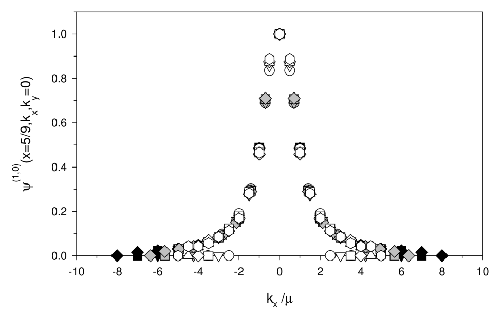
FIG. 1.: A cross section of the boson-fermion two-body amplitude taken at fixed longitudinal momentum fraction $x=5/9$ and at fixed $k_{y}=0$, with $K=9$, $\langle:\!\!\phi^{2}(0)\!\!:\rangle=1$, and $\mu_{1}^{2}=10\mu^{2}$. The cutoff $\Lambda^{2}$ and the transverse resolution $N_{\perp}$ are varied to keep the transverse scale $L_{\perp}$ fixed at one of the following values: $1\frac{\pi}{\mu}$ (black), $\sqrt{2}\frac{\pi}{\mu}$ (gray), and $2\frac{\pi}{\mu}$ (white). Different symbol shapes correspond to different values of $N_{\perp}$. The peaks are normalized to be equal at $k_{x}=0$. The points at zero amplitude mark the transverse range, which is set by the cutoff.

Calculations [5] have shown that the wave functions quickly become independent of $K$ and $L_{\perp}$ as these parameters are increased. The independence with respect to $L_{\perp}$ can be seen in Fig. 1. However, $F^{\prime}(0)$ was found to be sensitive to $L_{\perp}$, and one would expect the tail of $F_{1}$ to be sensitive to $\Lambda^{2}$ as well as $L_{\perp}$. That this is the case can be seen in Figs. 2 and 3. For small $\Lambda^{2}$ the form factor quickly reaches the bare-fermion contribution. For larger $\Lambda^{2}$ the bare-fermion contribution increases slightly, and the approach of $F_{1}$ to this limiting value becomes more gradual. When $\Lambda^{2}$ is large enough for the shape of $F_{1}$ to appear converged there remains a significant $L_{\perp}$ dependence, as seen in Fig. 3, even though the one-boson wave function changes little with $L_{\perp}$. The form factor remains sensitive because $L_{\perp}$ controls the approximation to the integral of the wave function product from which $F_{1}$ is computed.

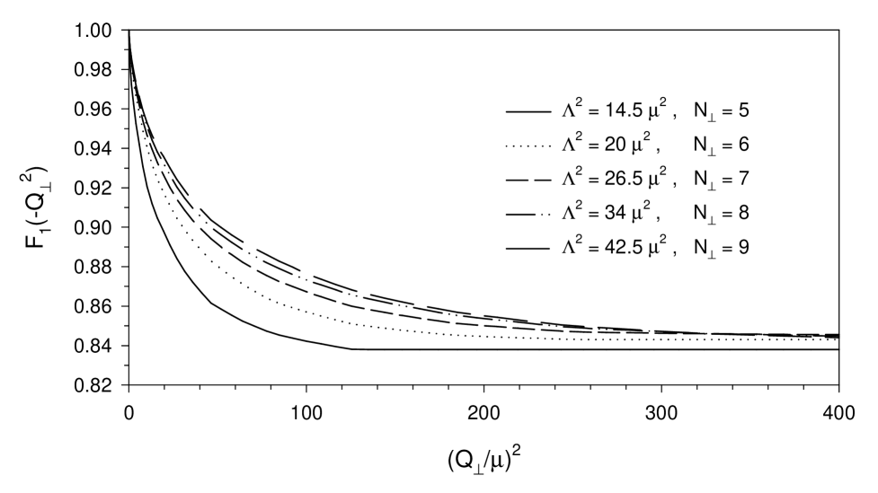
FIG. 2.: The form factor $F_{1}$ for fixed resolution $K=9$ and $L_{\perp}=2\pi/\mu$. Various cutoffs $\Lambda^{2}$ are considered. The model parameter values are $\langle:\!\!\phi^{2}(0)\!\!:\rangle=1$, $M^{2}=\mu^{2}$, and $\mu_{1}^{2}=10\mu^{2}$.

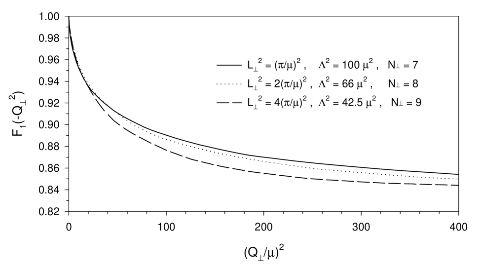
FIG. 3.: The form factor $F_{1}$ for fixed longitudinal resolution $K=9$ and varying transverse resolution $L_{\perp}$. The largest available cutoff was used in each case. The model parameter values are $\langle:\!\!\phi^{2}(0)\!\!:\rangle=1$, $M^{2}=\mu^{2}$, and $\mu_{1}^{2}=10\mu^{2}$.

V Summary

These results show that, at least for model Hamiltonians, a field-theoretic calculation of Fock-state wave functions and bound-state form factors can be carried out. The added Pauli–Villars particles provide the ultraviolet regularization without making the basis size unmanageable. Work on a more complete field theory, a single-fermion truncation of Yukawa theory, is underway. Consideration of the dressed-electron and positronium states of quantum electrodynamics would be a natural next step. QCD will require a more sophisticated approach, perhaps relying on heavy supersymmetric partners to play the role of the Pauli–Villars particles.

REFERENCES

[1] S.D. Drell and T.-M. Yan,
Phys. Rev. Lett. 24, 181 (1970).
[2] S.J. Brodsky and S.D. Drell,
Phys. Rev. D 22, 2236 (1980).
[3] H.-C. Pauli and S.J. Brodsky,
Phys. Rev. D 32, 1993 (1985); 32, 2001 (1985).
[4] S.J. Brodsky, J.R. Hiller, and G. McCartor,
Phys. Rev. D 58, 025005 (1998).
[5] S.J. Brodsky, J.R. Hiller, and G. McCartor,
Phys. Rev. D 60, 054506 (1999).
[6] W. Pauli and F. Villars,
Rev. Mod. Phys. 21, 4334 (1949).
[7] P.A.M. Dirac,
Rev. Mod. Phys. 21, 392 (1949).
[8] For a review of light-cone quantization and DLCQ, see
S.J. Brodsky, H.-C. Pauli, and S.S. Pinsky,
Phys. Rep. 301, 299 (1997).
[9] An alternative approach is to construct an
effective Hamiltonian perturbatively and diagonalize the
new Hamiltonian. For this see,
K.G. Wilson, T.S. Walhout, A. Harindranath,
W.-M. Zhang, R.J. Perry, and St.D. Głazek,
Phys. Rev. D 49, 6720 (1994);
St.D. Głazek and K.G. Wilson,
Phys. Rev. D 48, 5863 (1993); 49, 4214 (1994);
M. Brisudová and R.J. Perry,
Phys. Rev. D 54, 1831 (1996);
M. Brisudová and R.J. Perry, ibid. 54, 6453 (1996);
M. Brisudová, R.J. Perry, and K.G. Wilson,
Phys. Rev. Lett. 78, 1227 (1997);
B.D. Jones, R.J. Perry, and St.D. Głazek,
Phys. Rev. D 55, 6561 (1997);
B.D. Jones and R.J. Perry,
ibid., 7715 (1997).
[10] C. Lanczos,
J. Res. Nat. Bur. Stand. 45, 255 (1950);
J. Cullum and R.A. Willoughby,
in Large-Scale Eigenvalue Problems,
eds. J. Cullum and R.A. Willoughby,
Amsterdam: Elsevier, 1986, Math. Stud. 127, p. 193.