hep-ph/9909462
UCCHEP/3-99
FSU-HEP-990723
Gauge and Yukawa Unification in SUSY with Bilinearly Broken R–Parity

Abstract

In a supersymmetric model where R–Parity and lepton number are violated bilinearly in the superpotential, which can explain the solar and atmospheric neutrino problems, we study the unification of gauge and Yukawa couplings at the GUT scale. We show that bottom–tau Yukawa coupling unification can be achieved at any value of $\tan\beta$, and that the strong coupling constant prediction from unification of gauge couplings is closer to the experimental value compared with the MSSM. We also study the predictions for $V_{cb}$ in a Yukawa texture ansätze.

Bilinear R–Parity Violation (BRpV) has attracted a lot of attention lately [1, 2] due to its prediction for neutrino masses [3, 4] in connection with the recent results from SuperKamiokande [5], confirming the deficit of muon neutrinos from atmospheric neutrino data [6]. The simplest interpretation of the data is in terms of $\nu_{\mu}$ to $\nu_{\tau}$ flavour oscillations with maximal mixing and a mass squared difference of

$$\Delta m^{2}_{\mathrm{atm}}\approx 10^{-3}-10^{-2}\,\,{\mathrm{eV}}^{2}\,.$$ (1)

In addition, the solar neutrino experiments [7] imply the existence of another independent neutrino mass squared difference

$$\Delta m^{2}_{\mathrm{sun}} \approx 10^{-10}\,\,{\mathrm{eV}}^{2}\,(\mathrm{VO})$$

$$\Delta m^{2}_{\mathrm{sun}} \approx 10^{-6}-10^{-4}\,\,{\mathrm{eV}}^{2}\,(\mathrm{MSW})$$ (2)

where VO stands for Vacuum Oscillation solution and MSW for the Mikheyev–Smirnov–Wolfenstein solution [8]. The solar effect could be due to $\nu_{e}$ to $\nu_{\mu}$ oscillations.

The solar and atmospheric neutrino problems can be solved in the context of BRpV [9] where the superpotential

$$W=W_{\mathrm{Yuk}}-\mu\widehat{H}_{d}\widehat{H}_{u}+\epsilon_{i}\widehat{L}_{i}\widehat{H}_{u}$$ (3)

contains three terms that mix the three lepton superfields with the Higgs superfield responsible for the up–type quark masses. The three mixing terms violate R–Parity and lepton number and are proportional to parameters $\epsilon_{i}$ with units of mass.

The three neutrinos mix with the four neutralinos, and in a see-saw type of mechanism one of them acquire a mass at tree level and the other two remain degenerate and massless. In the case of $\epsilon_{1}\ll\mu,M_{1/2}$ the tree level neutrino mass can be approximated to [9, 10]

$$m_{\nu}\approx{{g^{2}M_{1}+g^{\prime 2}M_{2}}\over{4{\mathrm{det}}({\bf M}_{\chi^{0}})}}|\vec{\Lambda}|^{2}\,,$$ (4)

where $\Lambda_{i}=\mu v_{i}+v_{d}\epsilon_{i}$ and $v_{i}$ are the vev’s of the sneutrinos. The matrix ${\bf M}_{\chi^{0}}$ is the $4\times 4$ submatrix corresponding to the original neutralinos. It can be shown that the parameters $\Lambda_{i}\approx\mu^{\prime}v^{\prime}_{i}$ are directly proportional to the sneutrino vev’s $v^{\prime}_{i}$ in the basis where the $\epsilon_{i}$ terms have been removed from the superpotential.

In order to calculate reliable neutrino masses and mixings it is imperative to include one–loop corrections to the three generations [9, 11]. In this way, the degeneracy and masslessness of the lightest two neutrinos is lifted. The renormalized mass matrix has the form

$$M_{ij}^{pole} = M_{ij}^{\overline{DR}}(\mu_{R})+\frac{1}{2}\Big{(}\Pi_{ij}(p_{i}^{2})+\Pi_{ij}(p_{j}^{2})$$ (5)

$$- m_{\chi^{0}_{i}}\Sigma_{ij}(p_{i}^{2})-m_{\chi^{0}_{j}}\Sigma_{ij}(p_{j}^{2})\Big{)}\,.$$

where $\mu_{R}$ is an arbitrary scale and $\Pi_{ij}$ and $\Sigma_{ij}$ are self energies. The explicit scale dependence of the self energies is canceled by the implicit scale dependence of the tree level masses in the $\overline{DR}$ scheme. The averaged form of the renormalized mass matrix is necessary for explicit gauge independence. The loops include:

where $F^{+}$ are mixtures of charginos and charged leptons, $F^{0}$ are neutralinos and neutrinos, $S^{+}$ are charged Higgs and charged sleptons, and $F^{0}$ are neutral Higgs and sneutrinos.

We work in the general $R_{\xi}$ gauge, and to achieve explicit gauge invariance we need to include the tadpole graph for the Goldstone bosons into the self energies. There are five tadpole equations associated to the real parts of the two neutral Higgs and three sneutrinos:

$$V_{linear}=t_{d}Re(H^{0}_{d})+t_{u}Re(H^{0}_{u})+t_{i}Re(\tilde{\nu}_{i})\,.$$ (6)

The renormalized tadpoles are

$$t_{\alpha}=t^{0}_{\alpha}-\delta t^{\overline{DR}}_{\alpha}+T_{\alpha}(Q)=t^{0}_{\alpha}+T^{\overline{DR}}_{\alpha}(Q)$$ (7)

where $T^{\overline{DR}}_{\alpha}(Q)\equiv-\delta t^{\overline{DR}}_{\alpha}+T_{\alpha}(Q)$ are the finite one–loop tadpoles without the Goldstone contribution.

                      

Figure 1: Solar mass squared difference $\Delta m^{2}_{12}$ as a function of $\epsilon^{2}/|\Lambda|$. Lower values of $\Delta m^{2}_{12}$ corresponds to VO solution and high values to the MSW effect.

The solar mass squared difference $\Delta m^{2}_{\mathrm{sun}}=\Delta m^{2}_{12}$ is plotted in Fig. 1 as a function of $\epsilon/|\Lambda|$, where $\epsilon^{2}=\sum_{i}\epsilon_{i}^{2}$ and $\Lambda^{2}=\sum_{i}\Lambda_{i}^{2}$. Lower values of $\epsilon/|\Lambda|$ leads to VO solutions and large values to solutions with the MSW effect. Maximality of the atmospheric angle is found for $|\Lambda_{\mu}|\approx|\Lambda_{\tau}|$, and maximality of the solar angle is obtained if $\epsilon_{e}\approx\epsilon_{\mu}$, as long as $\Lambda_{e}$ is about a decade smaller than the other two.

An important consequence of the supersymmetric solutions to the neutrino problems is the necessity of $\tan\beta\raise 1.29167pt\hbox{$\;<$\kern-7.5pt\raise-4.73611pt\hbox{$\sim\;$}}10$, implying that the lightest Higgs boson mass satisfy $m_{h}\raise 1.29167pt\hbox{$\;<$\kern-7.5pt\raise-4.73611pt\hbox{$\sim\;$}}115$ GeV. In BRpV the neutral Higgs mix with the sneutrinos, and although this mixing does not affect the upper bound on $m_{h}$, it can reduce the mass in a few GeV [12]. A large part of the Higgs mass $m_{h}$ comes from radiative corrections near $\tan\beta=1$ [13] and therefore it is smaller than at high $\tan\beta$. This is the reason why LEP2 has started to prove this region of parameter space, preliminary ruling out $1\leq\tan\beta\raise 1.29167pt\hbox{$\;<$\kern-7.5pt\raise-4.73611pt\hbox{$\sim\;$}}1.8$ [14].

The analysis of BRpV with three massive neutrinos is very involved and for many applications it is enough to consider the one–generation approximation. In the study of gauge and Yukawa unification, the details of neutrino masses and mixing are not relevant, and for simplicity we consider BRpV only in the tau sector. The superpotential is the one in eq. (3) with $\epsilon_{1}=\epsilon_{2}=0$ and $\epsilon_{3}\neq 0$. in addition, an extra soft parameter $B_{3}$ is introduced

$$V_{\mathrm{soft}}^{\mathrm{BRpV}}=V_{\mathrm{soft}}^{\mathrm{MSSM}}+B_{3}\epsilon_{3}\tilde{L}_{3}H_{2}+h.c.$$ (8)

In this context, the tau neutrino acquire a mass at tree level given by

$$m_{\nu_{\tau}}\approx{{g^{2}}\over{2M}}v^{\prime 2}_{3}$$ (9)

where $v^{\prime}_{3}$ is the sneutrino vev in the basis where the $\epsilon_{3}$ term is removed from the superpotential. The tadpole equations allow us to find an approximated expression for this vev

$$v^{\prime}_{3}\approx-{{\epsilon_{3}\mu}\over{\mu^{\prime 2}m_{\tilde{\nu}^{0}_{\tau}}^{2}}}\left(v^{\prime}_{1}\Delta m^{2}+\mu^{\prime}v_{2}\Delta B\right)$$ (10)

where $\Delta m^{2}=m_{H_{1}}^{2}-m_{L_{3}}^{2}$ and $\Delta B=B_{3}-B$ are evaluated at the weak scale. In models with universal boundary conditions at the GUT scale, these two differences at the weak scale are radiativelly generated and proportional to the bottom Yukawa coupling squared.

The sneutrino vev $v_{3}$ contribute to the $W$ boson mass $m_{W}^{2}={\textstyle{1\over 4}}g^{2}(v_{u}^{2}+v_{d}^{2}+v_{3}^{2})$, therefore the Higgs vevs are smaller compared to the MSSM case. Because of this, although the relation between the quark masses and the Yukawa couplings does not change

$$m_{t}^{2}={\textstyle{1\over 2}}h_{t}^{2}v_{u}^{2}\,,\qquad m_{b}^{2}={\textstyle{1\over 2}}h_{b}^{2}v_{d}^{2}\,,$$ (11)

the numerical value of the Yukawas is different compared with the MSSM. The case of the tau Yukawa coupling is different due to the tau mixing with the charginos. The tau mass is

$$m_{\tau}^{2}={\textstyle{1\over 2}}h_{\tau}^{2}v_{d}^{2}(1+\delta)$$ (12)

where $\delta\geq 0$ depends on the parameters of the chargino–tau mass matrix [15].

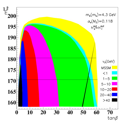
Figure 2: Top quark pole mass as a function of $\tan\beta$ for different values of the sneutrino vev $v_{3}$. Bottom–tau Yukawa unification in BRpV can be obtained at any value of $\tan\beta$. Top–bottom–tau unification (inclined line) is achieved at high $\tan\beta$ in a slightly wider region compared to the MSSM.

In this context we have made a complete scan over parameter space looking for solutions with bottom–tau Yukawa unification within $1\%$. In Fig. 2 we plot the top quark pole mass as a function of $\tan\beta$ differenciating the regions with the value of the sneutrino vev $v_{3}$ (there is some overlap between the regions that we do not show). The two horizontal lines correspond to the $1\sigma$ experimental determination of the top quark mass [16]. The MSSM case is also shown and the usual two solutions, one for large $\tan\beta\sim 55$ and one for small $\tan\beta\sim 2$, can be observed. As we can infer from the figure, bottom–tau Yukawa unification in BRpV can be achieved at any value of $\tan\beta$ provided we tune the value of $v_{3}$. In addition, top–bottom–tau Yukawa unification (inclined line) is achieved in a slightly wider region at high $\tan\beta$ [17].

To understand this result, consider the ratio between $h_{b}$ and $h_{\tau}$ at the weak scale. According to eqs. (11) and (12) this ratio is

$${{h_{b}}\over{h_{\tau}}}(m_{weak})={{m_{b}}\over{m_{\tau}}}\sqrt{1+\delta}$$ (13)

with $\delta$ increasing when $v_{3}$ departs from zero. In addition, solving the RGE’s with bottom–tau unification at the weak scale we get

$$\!\!\!\!\!\!\!\!\!\!\!\!{{h_{b}}\over{h_{\tau}}}(m_{weak})\approx$$

$$\!\!\!\!\!\!\!\!\!\!\!\!exp\left[{1\over{16\pi^{2}}}\left({16\over 3}g_{s}^{2}-3h_{b}^{2}-h_{t}^{2}\right)\ln{{M_{GUT}}\over{m_{weak}}}\right]$$ (14)

Comparing eqs. (13) and (14) we infer that the combination $3h_{b}^{2}+h_{t}^{2}$ decreases when $v_{3}$ departs from zero ($v_{3}=0$ corresponds to the MSSM).

      

Figure 3: Ratio between the top and bottom quark Yukawa couplings at the weak scale in the MSSM as a function of $\tan\beta$.

In Fig. 3 we plot the ratio $h_{t}/h_{b}$ as a function of $\tan\beta$ for the MSSM points corresponding to the outer band in Fig. 2. The points with acceptable $m_{t}$ (within $1\sigma$) and high $\tan\beta$ lie in the range $53\raise 1.29167pt\hbox{$\;<$\kern-7.5pt\raise-4.73611pt\hbox{$\sim\;$}}\tan\beta\raise 1.29167pt\hbox{$\;<$\kern-7.5pt\raise-4.73611pt\hbox{$\sim\;$}}60$ and in this reagion clearly $h_{b}$ dominates in the combination $3h_{b}^{2}+h_{t}^{2}$. If $v_{3}$ departs from zero (away from the MSSM) then $h_{b}$ decreases in order to achieved bottom-tau unification. In order to keep the bottom quark mass constant, the vev $v_{d}$ increases, and to keep the gauge boson masses constant the vev $v_{2}$ decreases, implying that unification is achieved in BRpV at smaller values of $\tan\beta$.

      

Figure 4: Ratio between the top and bottom quark Yukawa couplings at the weak scale in the BRpV as a function of $\tan\beta$ for $5<\tan\beta<10$ GeV.

In Fig. 4 we have the ratio $h_{t}/h_{b}$ as a function of $\tan\beta$ for BRpV with $5<v_{3}<10$ GeV. Looking at the figure we confirm that the region where $h_{b}$ dominates over $h_{t}$ in eq. (14) is at smaller values of $\tan\beta$, where $b-\tau$ unification and correct $m_{t}$ is achieved.

It is clear that bottom–tau unification in BRpV is controlled by the sneutrino vev $v_{3}$ and not directly by the neutrino masses. It is perfectly possible to have large effects in bottom–tau unification and a small tau neutrino mass, although the complete case with three neutrinos and masses calculated up to one–loop is under investigation.

Another interesting effect controlled, as we will see below, by the sneutrino vev $v_{3}$ are the predictions for $\alpha_{s}$ from unification of gauge couplings at the GUT scale [18]. The experimental world average of the strong coupling constant $\alpha_{s}(m_{Z})^{W.A.}=0.1189\pm 0.0015$ [19] is about $2\sigma$ lower than the GUT prediction in the MSSM [20], as we illustrate in Fig. 5.

 

Figure 5: Gauge coupling GUT unification prediction for $\alpha_{s}(m_{Z})$ as a function of the weak mixing angle $\sin^{2}\theta_{W}(m_{Z})$ in the MSSM.

In this figure we have made a scan over all parameter space in the MSSM–SUGRA including supersymmetric threshold corrections given by [20]

$$\Delta\alpha_{s}^{SUSY}=-\frac{19\alpha_{s}^{2}}{28\pi}\ln\left(\frac{T_{SUSY}}{\hbox{M}_{t}}\right)$$ (15)

where $T_{SUSY}$ is an effective mass scale given by

$$\!\!\!\!\!\!\!\!\!\!\!\!T_{SUSY}=m_{\widetilde{H}}\left({{m_{\widetilde{W}}}\over{m_{\tilde{g}}}}\right)^{28\over 19}\Bigg{[}$$

$$\!\!\!\!\!\!\!\!\!\!\!\!\left({{m_{\tilde{l}}}\over{m_{\tilde{q}}}}\right)^{3\over 19}\left({{m_{H}}\over{m_{\widetilde{H}}}}\right)^{3\over 19}\left({{m_{\widetilde{W}}}\over{m_{\widetilde{H}}}}\right)^{4\over 19}\Bigg{]}\,.$$ (16)

The $2\sigma$ difference is not a real discrepancy, nevertheless, it is interesting to compare it with the predictions for $\alpha_{s}$ in BRpV.

 

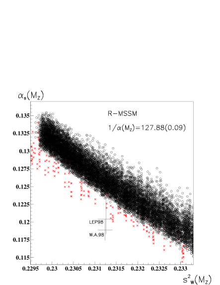
Figure 6: Gauge coupling GUT unification prediction for $\alpha_{s}(m_{Z})$ as a function of the weak mixing angle $\sin^{2}\theta_{W}(m_{Z})$ in BRpV.

With BRpV embedded into SUGRA with universality of soft masses at the GUT scale, where the gauge couplings unify, we have made a scan over parameter space looking for the prediction of $\alpha_{s}$ at the weak scale. The results are presented in Fig. 6 where we plot the strong coupling constant as a function of $\sin^{2}\theta_{W}(m_{Z})$. Interestingly, there is a $1\sigma$ improvement compared to the MSSM. This effect can be understood by noticing that the Yukawa couplings, which contribute to the running of $\alpha_{s}$ at the two–loop level, make a contribution to $\alpha_{s}$ that can be approximated by

$$\Delta\alpha_{s}^{YUK}\approx-\frac{\alpha_{s}^{2}}{32\pi^{3}}\ln\left(\frac{\hbox{M}_{U}}{\hbox{M}_{t}}\right)b_{3}^{\prime}\left\{h^{2}_{t}+h^{2}_{b}\right\}\,,$$ (17)

and the difference between BRpV and MSSM is that in the former case the combination $h_{t}^{2}+h_{b}^{2}$ can be larger than in the later case. From eq. (11) we get

$$h_{t}^{2}+h_{b}^{2}=2\left({{m_{t}^{2}}\over{v_{u}^{2}}}+{{m_{b}^{2}}\over{v_{d}^{2}}}\right)\,.$$ (18)

In the MSSM at high values of $\tan\beta$ both Yukawa couplings are comparable, the vev $v_{u}$ is very close to 246 GeV, and $v_{d}$ is just a few GeV. What happens in BRpV is that sneutrino vevs $v_{3}$ of only a few GeV (comparable to $v_{d}$) can lift the value of the bottom Yukawa coupling to twice as large, since to keep the gauge boson masses constant $v_{d}$ must decrease.

      

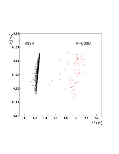
Figure 7: Strong coupling constant as a function of $h_{t}^{2}+h_{b}^{2}$ for points with lowest $\alpha_{s}$ for each value of $\sin^{2}\theta_{W}$ in both the MSSM and BRpV.

This effect can be seen in Fig. 7 where we plot the value of $\alpha_{s}(m_{Z})$ as a function of the combination $h_{t}^{2}+h_{b}^{2}$ for the points in Figs. 5 and 6 that lie in the lower part of each strip (the smallest values of $\alpha_{s}$ for each value of $\sin^{2}\theta_{W}$). We clearly observe the effect that $h_{t}^{2}+h_{b}^{2}$ is larger in BRpV than in the MSSM, reason why the BRpV prediction of $\alpha_{s}$ is closer to the experimental value.

Figure 8: Regions with acceptable values of $V_{cb}$ in the $\tan\beta-m_{top}$ plane for the MSSM.

The prediction of $V_{cb}$ in the simplest Yukawa texture ansätze [15] has been also studied. In this case, in addition to the GUT condition $h_{b}(M_{GUT})=h_{\tau}(M_{GUT})$ we impose the condition

$$\Big{|}V_{cb}(M_{GUT})\Big{|}=\sqrt{{h_{c}(M_{GUT})}\over{h_{t}(M_{GUT})}}$$ (19)

which is a prediction of the texture. We look for solutions satisfying the experimental constraint $0.036<|V_{cb}|<0.042$ at $90\%$ c.l. [21] . Solutions in the MSSM are in Fig. 8 imposing the two boundary conditions at the GUT scale within the percentage indicated by the figure. With GUT conditions at $5\%$ the large $\tan\beta$ solution for bottom–tau Yukawa unification disappears because it does not predict an acceptable value for $V_{cb}$. The large $\tan\beta$ solution reappears if we relax the GUT conditions, and it is fully present imposing them at $40\%$.

Figure 9: Regions with acceptable values of $V_{cb}$ in the $\tan\beta-m_{top}$ plane for BRpV.

In Fig. 9 we present the same analysis but for BRpV. First of all, the allowed region corresponding to GUT conditions at $5\%$ is slightly larger in BRpV. Indeed if we look only the region where $m_{t}$ is within $2\sigma$ of its experimental determination, the BRpV region is twice as large as in the MSSM [15]. More important differences between the two models appear when the GUT relations are relaxed: in BRpV it reappear the whole plane $m_{t}-\tan\beta$ as an allowed region when we relax the GUT conditions to $40\%$.

The fact that $V_{cb}$ predictions tend to cut solutions with high values of $\tan\beta$ (observed in the MSSM as well as BRpV) can be understood considering the RGE for the ratio between $|V_{cb}|$ and $R_{c/t}\equiv h_{c}/h_{t}$ [22]. Imposing the relation in eq. (19) at the GUT scale, we obtain at the weak scale

$${{R_{c/t}}\over{|V_{cb}|^{2}}}(m_{w})\approx exp\left[{1\over{16\pi^{2}}}\Big{(}h_{t}^{2}-h_{b}^{2}\Big{)}\ln{{M_{GUT}}\over{m_{weak}}}\right]$$ (20)

Since the left hand side of eq. (20) is greater than one (approximately equal to 1.5), it is clear that the GUT condition $R_{c/t}=|V_{cb}|^{2}$ prefers the region of parameter space where the top Yukawa coupling is large while the bottom Yukawa coupling is small. This is obtained at small values of $\tan\beta$.

BRpV has many other important phenomenological consequences. The most crucial one for collider physics is the decay of the lightest supersymmetric particle (LSP). This modifies all serach strategies for supersymmetric partners. Here we mention also constraints from the decay mode $b\rightarrow s\gamma$. It was shown that the constraints on the charged Higgs mass from the CLEO measurement for $B(b\rightarrow s\gamma)$ [23] in the MSSM [24] are relaxed in BRpV [25].

In summary, BRpV, which provides an explanation for the solar and atmospheric neutrino problems, achieves $b-\tau$ unification at any value of $\tan\beta$, predicts a value for $\alpha_{s}$ closer to the experimental value, and predicts the value of $V_{cb}$ in a wider region of parameter space, making it a serious alternative to the MSSM.

References

- [1] O.C.W. Kong, Mod. Phys. Lett. A14, 903 (1999); B. Mukhopadhyaya, S. Roy, and F. Vissani, Phys. Lett. B 443, 191 (1998); V. Bednyakov, A. Faessler, and S. Kovalenko, Phys. Lett. B 442, 203 (1998); E.J. Chun, S.K. Kang, C.W. Kim, and U.W. Lee, Nucl. Phys. B 544, 89 (1999); A. Faessler, S. Kovalenko, and F. Simkovic, Phys. Rev. D 58, 055004 (1998); A.S. Joshipura, S.K. Vempati, hep-ph/9808232; C.-H. Chang and T.-F. Feng, hep-ph/9901260; D.E. Kaplan and A.E. Nelson, hep-ph/9901254; T.-F. Feng, hep-ph/9806505.
- [2] M.A. Díaz, D.A. Restrepo, J.W.F. Valle, hep-ph/9908286; J. Ferrandis, hep-ph/9810371; A. Akeroyd, M.A. Díaz, and J.W.F. Valle, Phys. Lett. B 441, 224 (1998); A. Akeroyd et al., Nucl. Phys. B 529, 3 (1998).
- [3] A. Masiero, J.W.F. Valle, Phys. Lett. B 251, 273, (1990); J.C. Romão, C.A. Santos, J.W.F. Valle, Phys. Lett. B 288, 311 (1992); J.C. Romao, A. Ioannisian and J.W. Valle, Phys. Rev. D55, 427 (1997); J.C. Romão, J.W.F. Valle, Nucl. Phys. B 381, 87 (1992); M. Shiraishi, I. Umemura and K. Yamamoto, Phys. Lett. B313, 89 (1993); D. Comelli, A. Masiero, M. Pietroni and A. Riotto, Phys. Lett. B324, 397 (1994)
- [4] G. G. Ross, J.W.F. Valle, Phys. Lett. 151B 375 (1985); J. Ellis, G. Gelmini, C. Jarlskog, G.G. Ross, J.W.F. Valle, Phys. Lett. 150B:142,1985; C.S. Aulakh, R.N. Mohapatra, Phys. Lett. B119, 136 (1982); L.J. Hall and M. Suzuki, Nucl. Phys. B 231, 419 (1984); I.-H. Lee, Phys. Lett. B 138, 121 (1984); Nucl. Phys. B 246,120 (1984); A. Santamaria, J.W.F. Valle, Phys. Rev. Lett. 60 (1988) 397 and Phys. Lett. 195B:423,1987.
- [5] SuperKamiokande Coll., Y. Fukuda et al., Phys. Rev. Lett. 81, 1562 (1998) and Phys. Rev. Lett. 81, 1158 (1998).
- [6] IMB Coll., R. Becker-Szendy et al., Proc. Suppl. Nucl. Phys. B 38, 331 (1995); Soudan Coll., W.W.M. Allison et al., Phys. Lett. B 449, 137 (1999); MACRO Coll., M. Ambrosio et al., Phys. Lett. B 434, 451 (1998).
- [7] Homestake Coll., B.T. Cleveland et al., Aphys. J. 496, 505 (1998); GALLEX Coll., W. Hampel et al., Phys. Lett. B 447, 127 (1999); SAGE Coll., J.N. Abdurashitov et al., astroph/9907113; SuperK. Coll., Y. Fukuda et al., Phys. Rev. Lett. 81, 1158 (1998).
- [8] S.P. Mikheyev and A.Yu. Smirnov, Yad. Fiz. 42, 1441 (1985) [Sov. J. Nucl. Phys. 42, 913 (1985)] and Il Nuovo Cim. C9, 17 (1986); L. Wolfenstein, Phys. Rev. D 17, 2369 (1978).
- [9] J.C. Romão et al., hep-ph/9907499.
- [10] M. Hirsch and J.W.F. Valle, hep-ph/9812463.
- [11] R. Hempfling, Nucl. Phys. B 478, 3 (1996).
- [12] M.A. Díaz, J. Romão, and J.W.F. Valle, Nucl. Phys. B 524, 23 (1998).
- [13] M.A. Díaz and H.E. Haber, Phys. Rev. D 46, 3086 (1992).
- [14] ALEPH Collaboration, hep-ex/9908016.
- [15] M.A. Díaz, J. Ferrandis, and J.W.F. Valle, hep-ph/9909212.
- [16] CDF Coll., F. Abe et al., Phys. Rev. Lett. 74, 2626 (1995); D0 Coll., S. Abachi et al., Phys. Rev. Lett. 74, 2632 (1995).
- [17] M.A. Díaz, J. Ferrandis, J.C. Romão, J.W.F. Valle, Phys. Lett. B 453, 263 (1999).
- [18] M.A. Díaz, J. Ferrandis, J.C. Romão, J.W.F. Valle, hep-ph/9906343.
- [19] C. Caso et al., Eur. Phys. J. C3, 1 (1998).
- [20] P. Langacker and N. Polonsky, Phys. Rev. D 47, 4028 (1993); M. Carena, S. Pokorski and C.E.M. Wagner, Nucl. Phys. B 406, 59 (1993); P. Langacker and N. Polonsky, Phys. Rev. D 52, 3081 (1995).
- [21] Rev. Part. Phys., Eur. Phys. J. C3, 1 (1998).
- [22] V. Barger, M.S. Berger, and P. Ohmann, Phys. Rev. D 47, 1093 (1993).
- [23] CLEO Collaboration (M.S. Alam et al.), Phys. Rev. Lett. 74, 2885 (1995).
- [24] J.L. Hewett, Phys. Rev. Lett. 70, 1045 (1993); M.A. Díaz, Phys. Lett. B 304, 278 (1993) and Phys. Lett. B 322, 207 (1994); K. Chetyrkin, M. Misiak, and M. Münz, Phys. Lett. B 400, 206 (1997); M. Misiak, S. Pokorski, J. Rosiek, hep-ph/9703442 .
- [25] M.A. Díaz, E. Torrente-Lujan, and J.W.F. Valle, Nucl. Phys. B 551, 78 (1999); E. Torrente-Lujan, hep-ph/9907220.