Quasi-Fixed Points and Charge and Colour Breaking in Low Scale Models
Abstract:
We show that the current LEP2 lower bound upon the minimal supersymmetric standard model (MSSM) lightest Higgs mass rules out quasi-fixed scenarios for string scales between and GeV unless the heaviest stop mass is more than 2 TeV. We consider the implications of the low string scale for charge and colour breaking (CCB) bounds in the MSSM, and demonstrate that CCB bounds from and -flat directions are significantly weakened. For scales less than GeV these bounds become merely that degenerate scalar mass squared values are positive at the string scale.
DAMTP-1999-118
hep-ph/9909448
1 Introduction
For many years, string and unification scales were thought to be high ( GeV). The perturbative heterotic formulation of string theory had the fundamental string scale GeV close to GeV because of its constrained description of the gravitational interaction. The grand unification (GUT) scale was around GeV, motivated by the apparent convergence of the gauge couplings when they were evolved to this value. Recently however, attention has turned to models that have lower string and/or unification scales [1, 2, 3, 4, 5, 6] and this has raised some interesting questions to do with renormalisation group evolution of parameters.
The most immediate is of course whether gauge or Yukawa unification is still possible or even necessary with a lower string scale. One example that achieves gauge unification at the string scale [2] has the couplings experience power law ‘running’ [2, 4, 5] above a compactification scale due to the presence of additional Kaluza-Klein modes. A Kaluza-Klein spectrum with the same ratios of gauge beta functions as those in the MSSM leads to a logarithmic running up to the compactification scale with rapid power law unification taking place very rapidly thereafter [2]. An example that does not achieve gauge unification is ‘mirage’ unification [6]. In mirage unification the gauge couplings at the string scale receive moduli dependent corrections that behave as if there were continued logarithmic running above the string scale up to unification at the usual . ‘Mirage unification’ refers to this fictitious unification111Note that although there are problems with the particular string realisation of mirage unification in ref. [6], the idea may be realisable in other models and remains an interesting possibility..
A particularly attractive choice for the string scale (albeit one that is not immediately accessible to experiment) is GeV [3]. In this case the hierarchy between the weak scale and the Planck scale arises without unnaturally small ratios of fundamental scales. It was also noted in the first reference of [3] that GeV gives neutrino masses of the right order. We return to this model below and refer to it as the Weak-Planck (WP) model.
In this paper we consider two other related issues in the Minimal Supersymmetric Standard Model (MSSM),
| (1) |
with a low string scale. The first concerns the top quark Quasi-Fixed Point (QFP). The QFP is characterised by a focusing of some MSSM parameters to particular ratios as the renormalisation scale is decreased towards the top quark mass, [7, 10, 12]. Formally it is defined to be the point in parameter space where there is a Landau pole in the top Yukawa coupling at the string or GUT scale (whichever is the lower). In practice however this focusing behaviour can occur for a large but finite , still treat-able by perturbation theory. The coupling focusses to some value at independent of provided it is large enough. In low scale models, with their foreshortened logarithmic running, one naturally expects this behaviour to be very different. If the pole is at , we expect the quasi-fixed value of the top Yukawa at to be larger than for the usual GUT scale unification. Conversely, for a given value of top mass and at the weak scale the model will be further from the QFP for . We shall determine the QFP prediction for , on which experimental constraints from LEP2 can be brought to bear in order to empirically constrain assuming the QFP scenario. In particular, we consider the empirically derived lower bound upon the lightest CP-even MSSM Higgs mass, which in the canonical GUT scenarios has been shown to be a strong restriction upon the QFP scenario [12].
The second issue we consider is the possibility of minima that break charge and colour lying along and flat directions [10, 13, 14, 15, 16, 17, 18]. The constraints found by requiring that there be no such (CCB) minima are dependent on the distance from the QFP. They are most severe at the QFP itself [10, 15, 16] and indeed, in the usual MSSM at the QFP, CCB constraints exclude half the parameter space. With a lower string scale it seems likely that such constraints will generally be less restrictive for two reasons. First, a given point in (weak-scale) parameter space will be further from the QFP as noted above. Second, the CCB minima are generated radiatively when the mass-squared parameter for becomes negative. When there is a lower string scale there is less ‘room’ for a minimum to form at vacuum expectation values (VEVs) much greater than the weak scale. (More specifically, there are positive mass-squared contributions to the potential along the flat direction that become dominant at lower VEVs.) We shall demonstrate that this is indeed the case and that for the CCB constraint (at least along the and flat directions) is merely that scalar mass squared values are positive.
We will throughout be discussing these aspects by assuming that there is the standard logarithmic running of the MSSM upto a scale, , that we rather loosely refer to as the string scale. This scale may be much lower than . We define the QFP to be where the top Yukawa has a Landau pole at this point, since any variation in the Yukawa couplings above is expected to be drastically changed by string physics. As for the CCB bounds, we derive them on the soft breaking parameters at since this is close to the scale at which we expect the supersymmetry breaking parameters to be derived in any fundamental string model (although we will have more to say on this in due course).
2 The Quasi-Fixed MSSM
The QFP [7, 10, 12] constraint, i.e. that the top Yukawa coupling has a Landau pole at the string scale, gives important predictions in terms of the couplings and masses of supersymmetric particles [7, 10, 12]. We now examine the prediction for numerically, paying special attention to its dependence on the string scale. Fermion masses and gauge couplings are set to be at their central values in ref. [19] except for , which is varied to show the induced uncertainty. Below , we run using a 3 loop QCD1 loop QED effective theory with all superpartners integrated out.
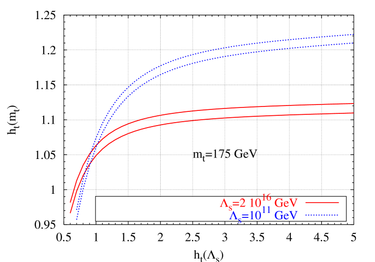
In order to illustrate the quasi-fixed behaviour we first make a rough calculation. To this end, we approximate the superparticle spectrum to be degenerate at , allowing us to use the (two-loop) MSSM renormalisation group equations above that scale. Fig. 1 illustrates the quasi-fixed behaviour for two values of string scale. The dependence of the low scale on its string scale value is shown for canonical QFP SUSY GUT framework with string/unification scale GeV. The almost horizontal part of the lines represent the QFP regime: where, for input values ,
| (2) |
results. Lowering to GeV, as in the WP model, we see that the quasi-fixed behaviour is diminished somewhat, as indicated by the more positive slope of the relevant lines. However, for a QFP value of
| (3) |
occurs222Errors quoted here include those due to the error in but they do not include those from non-degeneracy in the superparticle spectrum..
The QFP prediction can be turned into a prediction of the MSSM parameter (the ratio of the two neutral Higgs VEVs) through the relation
| (4) |
and the known value [19] of the top quark mass, GeV. We obtain the running top mass from by employing the 1-loop QCD correction, thus assuming that supersymmetric corrections to it are small. refers to the Standard Model Higgs VEV of 246.22 GeV. Low values of result from eq. (4) when a quasi-fixed value is used. The range of relevant here is constrained by the non-observation of the lightest MSSM Higgs boson at LEP2 [12]. The current limits [20] exclude GeV for the low scenario. Quasi-fixed predictions are illustrated in table 1, where they are displayed with estimated uncertainties for the WP and GUT quasi-fixed scenarios. The uncertainties are induced by those quoted in the predictions in Eqs. (2),(3).
| (GeV) | GeV | GeV |
|---|---|---|
Here, we set , close to its Landau pole and near the edge of perturbativity. In ref. [21], the limit was used to define a perturbative regime and we will use the point as an estimator of sensitivity to . A central value of [19] was used. We display the results for GeV to illustrate the large dependence upon the top mass. We use the two-loop diagrammatic result in ref. [22] to calculate the MSSM lightest Higgs mass with the state-of-the-art program FeynHiggsFast2. Corrections to the values of displayed in fig. 1 from including sparticle thresholds are expected to be small because the majority of change in occurs in the running between and 1000 GeV, identical in both cases. We therefore use the prediction for as calculated with a degenerate sparticle spectrum at . To within small errors, this value should still be applicable for a non-degenerate spectrum, which is what we assume here.
Ideally, we would now perform a parameter scan through the low energy supersymmetry breaking parameters in order to determine the maximum value of consistent with the QFP. This is impractical however, and we resort to using a benchmark point in low energy supersymmetry breaking parameter space. The value of obtained by the benchmark corresponds in practice to be very close (within one GeV) to a more general upper bound on [22], given an upper bound on sparticle masses. For generality, this benchmark corresponds to non-universal SUSY breaking parameters. For a given value of , is predicted by the QFP as in Fig. 1. We then set and the parameter
| (5) |
As is argued in [22], corresponds to the maximal-mixing case, where is maximised. is then specified by eq 5, and therefore the gluino mass will be set by the QFP prediction of . For GeV for example, we obtain [10]. However to the order in perturbation theory used here, the Higgs mass is independent of the gluino mass. Fixing then sets through the relation [11]
| (6) |
The two electroweak symmetry breaking conditions are [11]
| (7) |
where plus loop corrections. Together, they determine the Higgs mass soft breaking parameters and (conservatively assumed to be uncorrelated and free). Following the authors of ref. [22], the maximum value of is assumed to be acquired by taking333See ref. [22] for a definition of these parameters. GeV, GeV, GeV and GeV in order to get a conservative estimate. Dependence of the upper bound on is logarithmic in this parameter and therefore slowly increasing as increases. Therefore, to obtain a sizeable effect on the bound, unnaturally high values of would have to be taken. Using the above procedure, the soft breaking parameters that depends most sensitively upon are fixed near the weak scale without reference to any further unification assumptions, such as minimal supergravity for example.
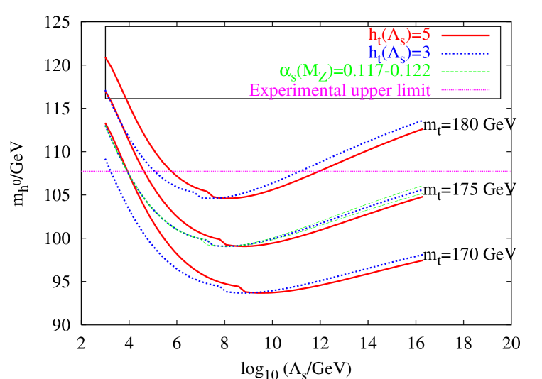
Fig. 2 displays the QFP value of predicted by the benchmark by varying . Uncertainties induced by the error on are shown for one particular case. It is larger for higher , but always less than 0.5 GeV and much smaller than the uncertainty induced by the empirical error on . In fact, we see from the figure that the QFP is ruled out to better than 1 for the range
| (8) |
for GeV and . If we take GeV, the QFP is ruled out for any GeV. As noted above, the curves give an estimate of the uncertainty in the QFP prediction. The figure shows that this dependence is small for GeV but that it increases for GeV. However, we note that in this latter range, being less than 5 (but still in the quasi-fixed regime) actually strengthens the upper bound upon . thus gives a reasonably accurate bound for GeV and a conservative one for GeV.
3 Analytic CCB Bounds at low string scales
We now turn to the discussion of CCB bounds. Unphysical CCB minima present some of the most severe bounds for supersymmetric models [13, 14, 10, 15, 16, 17, 18]. Indeed, for a number of models it has been found that they exclude much of the parameter space not already excluded by experiment; for example the MSSM where supersymmetry breaking is driven by the dilaton [14], SUSY GUTS at the low quasi-fixed point (QFP) [10], -theory in which supersymmetry breaking is driven by bulk moduli fields [16, 17] and several other string/field theory scenarios [17, 18]. All of the above work, however, assumed a logarithmic evolution of the gauge couplings with unification at a high scale GeV.
In this section we shall be considering the effect of truncating this logarithmic evolution at a low string scale. For completeness, we first recall the three types of CCB minima that can occur in supersymmetric models:
-
•
-flat directions which develop a minimum due to large trilinear supersymmetry breaking terms.
-
•
and flat directions corresponding to a single gauge invariant.
- •
Since the first type are important at low scales [13] and the second type are only important when there are negative mass-squared terms at the GUT scale, we shall concentrate on the constraints coming from the last type of minimum. These occur at intermediate scales due to the running mass-squared even if all the mass-squared values are positive at the GUT scale. Hence the resulting constraints are very dependent on renormalisation group running at high scales and are particularly interesting from the point of view of models with a lower string scale. As discussed above, our initial expectation is that the CCB bounds will be far less severe than in the usual versions of the MSSM.
We will consider the and -flat direction in the MSSM corresponding to the operators
| (9) |
where the suffices on matter superfields are generation indices. With the following choice of VEVs;
| (10) |
the potential along this direction depends only on the soft supersymmetry breaking terms (neglecting a small D-term contribution);
| (11) |
In the usual MSSM we can reasonably assume that, since the CCB minimum forms at VEVs corresponding to , the largest relevant mass, and therefore the appropriate scale to evaluate the parameters at, is . This minimises the top quark contributions to the effective potential at one-loop. Further corrections to the potential are assumed to be small. Once we lower the string scale however we encounter the problem that the CCB minimum moves towards low scales and that consequently this approximation breaks down. Evidently, from eq. (11), this happens precisely where the positive terms begin to dominate, and so we do not anticipate that CCB minima will be formed when . In order to check this however, our approach will be to construct the constraints using the above assumption on and observe that they get far less restrictive as we move to moderately low string scales, say . We then check the approximate one-loop analytic results obtained with a more accurate two-loop numerical analysis at certain parameter points and observe numerically that CCB minima do not reappear as we move to very low string scales where .
In the above potentials, so that the eq. (11) is of the form
| (12) |
where , is the combination of mass-squared parameters (also evaluated at ) that appears in the potential,
| (13) |
and is an arbitrary scale which we shall take to be the usual unification scale . The bound is therefore governed by , and the parameter
| (14) |
for the direction described above, or
| (15) |
for the equally dangerous direction.
To estimate the bound, we now adapt the results of Refs.[15, 16]. At large values of the potential is governed by the first term. Whatever the string scale may be, we require that be positive there and negative at (for successful electroweak symmetry breaking). A CCB minimum radiatively forms close to the value where first becomes negative (typically at a scale of ) [15, 16].
In Refs.[15, 16] it was shown that once we are able to estimate the bound follows fairly easily, and this was done for models with degenerate gaugino masses. Bounds were derived for all non-universal scalar masses and couplings. In the present case however, the gauge couplings and the gaugino masses are also non-degenerate at the string scale .
This makes a general analytic treatment of the RGEs extremely difficult, so in order to simplify matters we shall henceforth assume the ‘GUT gaugino relation’. That is we assume that at the scale we have the usual GUT expression for gaugino masses,
| (16) |
This relationship has the useful property that the gaugino masses as well as the gauge couplings would be degenerate if we continued the evolution of the MSSM RGEs upto . We shall call this fictitious degenerate value . Note that eq. (16) is only valid to one-loop order, and indeed in this section we present analytic results to one-loop order only (contrary to the last section).
Although eq.(16) may seem like a rather brutal requirement, it holds for a number of interesting cases, for instance in models with power law unification as shown in ref. [5]. In these models the scale in our analysis should really be interpreted as the compactification scale at which the first Kaluza-Klein states appear in the spectrum, rather than the string scale which is where we expect the real gauge unification to take place after a short period of power law ‘running’. An assumption such as degenerate soft terms at the compactification scale is consistent with, for example, the Scherk-Schwarz mechanism of supersymmetry breaking.
Eq.(16) is also expected to hold in the mirage unification models of ref.[6] when there is no -mixing and in the limit . In this limit we have
| (17) |
where we use the subscript-0 to represent values at the usual unification scale (i.e. ), and where we have neglected terms of order which is consistent to one-loop accuracy. In this case we have .
Eq.(16) allows us to adapt the expressions of ref.[15] with only a modest amount of effort by writing the parameters at in terms of their values at . In order to proceed, we next spend a little time discussing the analytic solutions to the renormalisation group running. The solutions of all the parameters may easily be expressed in terms of those combinations with infra-red QFPs; , and . These may be written as functions of
| (18) |
so that
| (19) |
Taking means that with corresponding to the GUT scale. If the string scale is at as in the WP model, then the corresponding value of is . It is useful to define
| (20) |
Solving for in terms of its value at the string scale (we use subscript- to denote string-scale values) we find
| (21) |
where the QFP value (where the Yukawa couplings blow up at the string scale) is given by
| (22) |
We also, for later use, define the distance from the real QFP,
| (23) |
This can be rewritten in terms of a fictitious renormalisation of down from a scale value of ; i.e. defining
| (24) |
we have
| (25) |
This is the usual expression for (c.f. ref.[16]); however it should be noted that is here merely a parameter that is negative in the region . In the usual MSSM with unification at the GUT scale, this would of course be an unphysical (non-perturbative) region. For and we now define the distance from the usual QFP (i.e. where couplings blow up at the usual unification scale )
| (26) |
and also
| (27) |
We then obtain expressions for and in terms of their fictitious values, and , at ;
| (28) |
where
| (29) |
It is important to note that, since
| (30) |
and retain their QFP behaviour since when (or ) they are both independent of their values at the string scale, . In addition, factors of cancel so that there is no divergent behaviour at the usual QFP. Also note that this QFP is at lower than in the usual MSSM unification. We can estimate the difference in at the QFP by using
| (31) |
so that
| (32) |
Eqs. (22,24) then give in the WP model with , in agreement with the full two-loop numerical result presented in fig. 1.
With all parameters expressed in terms of GUT scale parameters, we are now simply able to apply the bounds derived in ref.[16] for non-universal SUSY breaking directly. Consider for example the , direction. The cosmological bounds in this case are
| (33) |
where is the value of at the scale and
| (34) |
for . (The small dependence of and on , which we must choose by hand, is discussed in ref.[16].) To a good approximation the value of is given by [16]
| (35) |
In order to relate the quantities to their string scale values, we use the one loop RGE solutions for and ;
| (36) | |||||
where
| (37) |
and where
| (38) |
The general behaviour of the bounds is clearly similar to that in the usual unification scenario. The bounds are on the particular combination and are most restrictive at the QFP, decreasing as increases. Away from the QFP there is a quadratic dependence on with a minimum at .
We can now see why the bounds at low scales are far less severe than in the MSSM with unification at the GUT scale. First, close to the QFP, the bound is
| (39) | |||||
for . Thus the non-degeneracy of gauge couplings and gauginos contributes negatively to the bound even at the QFP. Second, away from the QFP, the bound asymptotes to the values with
| (40) |
However, the quantity multiplying in the bound is now which is a larger negative factor than .
We now further specialise to the mirage unification models with , which have degenerate -terms and degenerate scalar masses at the string scale;
| (41) |
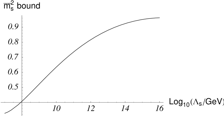
Contours of the , bound are shown in fig. 3, for varying and . The diagram shows that a lower string scale removes the dangerous minima. Indeed, for the WP model value of , there are no CCB minima appearing along the , direction except close to the QFP () or for negative scalar mass squared values (). At the QFP we find that the bound at GeV is but drops rapidly towards smaller values of , as shown in fig. 4. A full numerical determination of the bounds for specific points in parameter space is in accord with Figs. 3 and 4. It also shows that the bounds are in fact not overly sensitive to the precise values of and at since the running is dominated by .
Moreover, this behaviour is expected to be a general feature resulting from the low string scale pushing the CCB minimum to low scales. For example we can analyse the bound at large where eq. (40) holds. Choosing and adjusting to make , one finds that, away from the QFP, there are no CCB minima for any positive choice of non-universal mass-squared parameters at the string scale for . In other words, for these intermediate and low string scales one may always adjust to remove CCB minima. Conversely, choosing a large enough value of forms a CCB minimum at any .
For the analytic approximations we have been using break down for reasons outline above. Specifically, instead of evaluating the parameters at the renormalisation scale , it is now more accurate to evaluate them at the scale (in the direction) since this would be the largest relevant mass. Using this definition for we find numerically that minima do not reappear when is lowered still further, as expected due to the dominance of the positive contribution to the potential at low VEVs.
4 Summary
To summarise, we have examined constraints on the MSSM coming from the QFP scenario and CCB bounds when the string scale is lower than the canonical unification value of GeV. The quasi-fixed behaviour is weakened somewhat as the scale is reduced, i.e. weak MSSM parameters retain more information about their high energy boundary conditions. Very strict bounds upon the string scale are obtained from the LEP2 lower bound upon the lightest Higgs mass in the QFP scenario. Current limits exclude the QFP scenario for string scales between and GeV for GeV. This range of exclusion will increase by the end of running of LEP2, as the bounds improve. Run II of the Tevatron is expected to decrease the errors upon significantly, with important implications for the range of ruled out in the quasi-fixed scenario. For example, an error of 1 GeV upon would rule out the QFP scenario for all GeV.
CCB bounds also give important constraints upon the quasi-fixed scenario. We provided an analytic treatment of CCB bounds with lower string scales which we confirmed with a more accurate numerical check. It is clear from our results that lowering the string scale significantly weakens the CCB bounds. As an example, we considered the most restrictive case of the QFP. In this case the lower bound upon string-scale, degenerate, scalar mass-squared values is weakened by 30% in the WP model, GeV. Remarkably, for and GeV, the CCB bound is merely for any non-universal pattern of supersymmetry breaking.
Although we have concentrated on a particular subset of models (i.e. those that preserve the ‘GUT gaugino relation’), we argue that our conclusions are true in a more general case. As the string scale is lowered, provided that all mass-squared values are initially positive, the CCB minima are inevitably pushed to lower VEVs. At these low scales, the negative term no longer dominates the potential along the most dangerous and -flat directions.
Acknowledgments.
This work was partially supported by PPARC. We would like to thank T. Gherghetta, L. Ibanez and F. Quevedo for helpful discussions. BCA would like to thank the CERN theory division (where this work was initiated) for hospitality offered.References
- [1] I. Antoniadis, Phys. Lett. B 246 (1990) 337; I. Antoniadis, C. Muñoz and M. Quirós, Phys. Lett. B 397 (1993) 515; P. Hořava and E. Witten, Nucl. Phys. B 460 (1996) 506; J. D. Lykken, Phys. Rev. D 54 (1996) 3697; N. Arkani-Hamed, S. Dimopoulos and G. Dvali, Phys. Lett. B 429 (1998) 263; I. Antoniadis, N. Arkani-Hamed, S. Dimopoulos and G. Dvali, Phys. Lett. B 436 (1998) 257
- [2] K. R. Dienes, E. Dudas and T. Gherghetta,Phys. Lett. B 436 (1998) 55; Nucl. Phys. B 537 (1999) 47
- [3] K. Benakli, hep-ph/9809582; C. P. Burgess, L. E. Ibáñez and F. Quevedo, Phys. Lett. B 447 (1999) 257
- [4] M. Lanzagorta and G. G. Ross, Phys. Lett. B 349 (1995) 319; D. Ghilencea and G. G. Ross, Phys. Lett. B 442 (1998) 165; S. A. Abel and S. F. King, Phys. Rev. D 59 (1999) 095010; I. Antoniadis, S. Dimopoulos, M. Quirós and A. Pomarol, Nucl. Phys. B 544 (1999) 503; T. Kobayashi, J. Kubo, M. Mondragon and G. Zoupanos, Nucl. Phys. B 550 (1999) 99; A. Delgado, A. Pomarol and M. Quirós, hep-ph/9812489
- [5] T. Kobayashi, J. Kubo, M. Mondragon and G. Zoupanos, Nucl. Phys. B 550 (1999) 99
- [6] L. E. Ibáñez, hep-ph/9905349
- [7] B. Pendleton and G. G. Ross, Phys. Lett. B 98 (1981) 21; C. T. Hill, Phys. Rev. D 24 (691) 1981, C. T. Hill, C. N. Leung and S. Rao, Nucl. Phys. B 262 (1985) 517; V. Barger, M. S. Berger, P. Ohmann and R. J. N. Phillips, Phys. Lett. B 314 (1993) 351; W. A. Bardeen, M. Carena, S. Pokorski and C. E. M. Wagner, Phys. Lett. B 320 (1994) 110; M. Lanzagorta and G. G. Ross, Phys. Lett. B 364 (1995) 163; M. Carena and C. E. M. Wagner, Nucl. Phys. B 452 (1995) 45; B. C. Allanach and S. F. King, Nucl. Phys. B 473 (1996) 3; S. A. Abel and B. C. Allanach, Phys. Lett. B 415 (1997) 371; G. K. Yeghian, M. Jurcisin and D. I. Kazakov, Mod. Phys. Lett A14 (1999) 601
- [8] S. Heinemeyer, W. Hollik and G. Weiglein, Phys. Lett. B 455 (1999) 179; Eur. Phys. J. C9 (1999) 343.
- [9] B. C. Allanach et al, Proceedings of Beyond the Standard Model Working Group, 1999 Durham Collider Workshop, J. Phys. G: Nucl. Part. Phys. 26 (2000) 1, hep-ph/9912302.
- [10] S. A. Abel and B. C. Allanach, Phys. Lett. B 431 (1998) 339
- [11] H.E. Haber, Boulder TASI 92 (1992) 0589
- [12] J. A. Casas, J. R. Espinosa and H. E. Haber, Nucl. Phys. B 526 (1998) 3
- [13] J. -M. Frère, D. R. T. Jones and S. Raby, Nucl. Phys. B 222 (1983) 11; M. Claudson, L. Hall and I. Hinchcliffe, Nucl. Phys. B 228 (1983) 501; H. -P. Nilles, M. Srednicki and D. Wyler, Phys. Lett. B 120 (1983) 346; J-P. Derendinger and C. A. Savoy, Nucl. Phys. B 237 (1984) 307; H. Komatsu, Phys. Lett. B 215 (1988) 323; P. Langacker and N. Polonsky, Phys. Rev. D 50 (1994) 2199; A. Kusenko, P. Langacker and G. Segré, Phys. Rev. D 54 (1996) 5824; J. A. Casas and S. Dimopoulos, Phys. Lett. B 387 (1996) 107; J. A. Casas, hep-ph/9707475; J. A. Casas, A. Lleyda and C. Muñoz, Nucl. Phys. B 471 (1996) 3; J. A. Casas, A. Lleyda and C. Muñoz, Phys. Lett. B 389 (1996) 305; H. Baer, M. Brhlik, D. Castano, Phys. Rev. D 54 (1996) 6944; T. Falk, K. A. Olive, L. Roszkowski and M. Srednicki, Phys. Lett. B 367 (1996) 183; A. Riotto and E. Roulet, Phys. Lett. B 377 (1996) 60; A. Strumia, Nucl. Phys. B 482 (1996) 24; T. Falk, K. A. Olive, L. Roszkowski, A. Singh and M. Srednicki, Phys. Lett. B 396 (1997) 50; S. Abel and T. Falk, Phys. Lett. B 444 (1998) 427; I. Dasgupta, R. Rademacher and P. Suranyi, Phys. Lett. B 447 (1999) 284; U. Ellwanger and C. Hugonie, Phys. Lett. B 457 (1999) 299
- [14] J. A. Casas, A. Lleyda and C. Muñoz, Phys. Lett. B 380 (1996) 59
- [15] S. A. Abel and C. A. Savoy, Nucl. Phys. B 532 (1998) 3
- [16] S. A. Abel and C. A. Savoy, Phys. Lett. B 444 (1998) 119
- [17] J. A. Casas, A. Ibarra and C. Muñoz, hep-ph/9810266
- [18] A. Dedes and A. E. Faraggi, hep-ph/9907331
- [19] C. Caso et al, Eur. Phys. Jnl. C3 (1998) 1
- [20] P. Texeira-Diaz, talk at “IoPHEP2000”
- [21] V. Barger, M.S. Berger and P. Ohmann, Phys. Rev. D 47 (1993) 1093
- [22] S. Heinemeyer, W. Hollik and G. Weiglein, hep-ph/9909540
- [23] J.A. Casas, A. Lleyda and C. Munoz, Nucl. Phys. B 471 (1996) 3
- [24] F. Buccella, J-P. Derendinger, C. A. Savoy and S. Ferrara, Phys. Lett. B 115 (1982) 375; R. Gatto and G. Sartori, Phys. Lett. B 157 (1985) 389; M. A. Luty and W. Taylor, Phys. Rev. D 53 (1996) 3399