hep-ph/9909445
POLARISATION IN
DEEPLY VIRTUAL MESON PRODUCTION

We discuss two aspects of polarisation in hard exclusive meson production: the leading-twist selection rule for the meson helicity, and the different partial waves of a $\pi\pi$-pair which may or may not be due to the decay of a $\rho$.

1 Helicity in vector meson production

The first half of this talk is about exclusive electroproduction of a $\rho$ (or any other light vector meson), $ep\to ep+\rho$, in the Bjorken limit where the photon virtuality $Q^{2}=-q^{2}$ becomes large, while $x_{B}=Q^{2}/(2p\cdot q)$ and the invariant momentum transfer $t=(p-p^{\prime})^{2}$ remain fixed. There is a factorisation theorem $\!{}^{{\bf?}}$ stating that in this limit the $\gamma^{*}p$ amplitude factorises into a hard photon-parton scattering and non-perturbative quantities, namely skewed quark and gluon distributions in the proton and a $q\bar{q}$ distribution amplitude of the meson. This is shown in Fig. 1, where also four-momenta are defined.

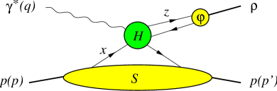
Figure 1: Factorisation of exclusive $\rho$-production into a hard-scattering coefficient $H$, a skewed quark distribution $S$ and a meson distribution amplitude $\varphi$. There are also diagrams with the skewed gluon instead of the quark distribution. $x$ and $z$ denote momentum fractions in the proton and the $\rho$, respectively.

The factorisation theorem provides a solid basis for extracting information on the quark and gluon structure of hadrons from this process, in particular for measuring skewed parton distributions. The description of the amplitude in terms of these quantities is of course only accurate up to power corrections in $1/Q$, and in a data analysis it is essential to investigate how close one is to the asymptotic regime at a given value of $Q^{2}$. It is at this point that helicity selection rules are of great value.

An essential part of the factorisation theorem is that the description of Fig. 1 only holds if the photon is longitudinally polarised in the $\gamma^{*}p$ c.m. The corresponding amplitude has a scaling behaviour ${\mathcal{A}}(\gamma^{*}_{L}p)\sim{\mathrm{c}onst}/Q$ in the Bjorken limit. For a transverse photon factorisation cannot be established since the loop integrals in the relevant Feynman graphs are sensitive to dangerous infrared regions, but the theorem predicts the corresponding amplitude to be suppressed by at least one power, ${\mathcal{A}}(\gamma^{*}_{T}p)\sim{\mathrm{c}onst}/Q^{2}$.

It turns out that there is a second selection rule, stating that to leading power in $1/Q$ one can only produce a longitudinal vector meson, while transverse $\rho$ production is again power suppressed. Collins, Frankfurt and Strikman $\!{}^{{\bf?}}$ observed that a transition $\gamma^{*}_{L}p\to\rho_{T}^{\phantom{*}}p$ at order $1/Q$ must involve the so-called chiral-odd quark distribution in the proton and the chiral-odd distribution amplitude of the $\rho$. This was promising given that experimental information on these quantities is very scarce. Unfortunately, the corresponding hard-scattering coefficient $H$ was found to be zero to lowest order in the strong coupling.$\!{}^{{\bf?}}$ A general symmetry argument shows that it is in fact zero to all orders in $\alpha_{s}$.$\!{}^{{\bf?}}$

Let us see what goes into this argument. The first ingredient is that the leading power behaviour of the diagrams in Fig. 1 is obtained by replacing the relative transverse momenta of the partons with zero when evaluating the hard scattering $H$. The hard subprocess is therefore collinear, say along the $z$-axis. The loop integral over the transverse momenta is performed in the soft quantities $S$ and $\varphi$ alone, and from rotation invariance it is easy to see that in $\varphi$ the helicities of the quark and antiquark must add up to the helicity of the meson. For a transverse $\rho$ this gives a chiral-odd distribution amplitude, i.e., one where $q$ and $\bar{q}$ have opposite chirality and thus equal helicity. The second ingredient is that when calculating to leading-power accuracy one can set the quark mass to zero in $H$. Then the hard scattering conserves quark helicity and thus selects the chiral-odd quark distribution in the proton target; chiral-even quark distributions and the gluon distribution do not contribute. When one follows the flow of helicity from the incoming to the outgoing quark lines in the Feynman graphs for $H$ one finds that the angular momentum along the $z$-axis changes by two units, a mismatch that cannot be compensated by the photon polarisation. Thus one finds $H=0$.

The previous argument did not take into account that at higher orders in $\alpha_{s}$ the Feynman diagrams for $H$ have infinities, so that one must first regularise them, then perform appropriate subtractions of these divergences, and finally remove the regularisation. Now, as soon as one regularises the theory, chirality is no longer conserved. Chirality breaking terms can survive even after the regularisation has been removed again, which gives for instance rise to the axial anomaly in QCD. Hoodbhoy and Lu $\!{}^{{\bf?}}$ have calculated the one-loop diagrams for $H$ and found indeed a non-zero result.

Their result is however incomplete since it misses the subtractions of collinear divergences that have to be made in the calculation of a hard-scattering coefficient $H$; if these are included one will find $H=0$ again. One can in fact give a general proof  $\!{}^{{\bf?}}$ that to any finite order in perturbation theory the hard-scattering coefficient conserves the chirality of its external quark lines, so that the symmetry argument sketched above is valid. The idea of the proof is to regularise the theory by going to $4-\epsilon$ dimensions, perform all subtractions of divergences and then set $\epsilon=0$, leaving the helicities of the external quarks in $H$ unspecified. The final result for $H$ lives in 4 dimensions, where chirality conservation it ensured by having an odd number of Dirac matrices $\gamma^{\mu}$ along each quark line. The latter is a consequence of the Feynman rules of massless QCD and is not invalidated by any of the intermediate steps in $4-\epsilon$ dimensions.

An alternative would be to use Pauli-Villars regularisation to render the loop integrals finite. Then chirality remains conserved along massless fermion lines. Only in internal quark loops do massive regulator fermions occur whose chirality is not conserved; this leads for instance to the axial anomaly in the triangle diagram of two vector and one axial current. It does, however, not disturb the fact that chirality is conserved for the external quark lines of $H$, which remain massless.

It is important to note that the argumentation leading to our helicity selection rule is very similar to the one that establishes hadron helicity conservation for exclusive processes at leading twist.$\!{}^{{\bf?}}$ The proof that a hard-scattering coefficient in perturbative QCD conserves chirality carries over to this case.

In summary, we have that the only leading-twist helicity amplitude is the one for $\gamma^{*}_{L}p\to\rho_{L}^{\phantom{*}}p$. All others must be due to power corrections. As the angular distributions in $ep\to ep+\rho\to ep+\pi^{+}\pi^{-}$ contain detailed information on the various helicity transitions, their study can give valuable information on how far one is from the asymptotic regime where the helicity selection rules apply.

Beyond this they may guide theory in describing the physics of power corrections itself, a field where we are far yet from a systematic theory. A crucial ingredient in deriving our selection rule was the collinearity of the hard scattering subprocess, and as soon as one keeps transverse parton momenta (and hence $t$) finite there, all helicity combinations appear. The relevance of the transverse momentum distribution of partons within hadrons has been emphasised in several papers dealing with the helicity structure of meson production in the small-$x_{B}$ regime,$\!{}^{{\bf?},{\bf?},{\bf?}}$ where increasingly accurate data are becoming available.$\!{}^{{\bf?}}$ Another important question is that of perturbative control over infrared regions in the loop integrals, to which the different helicity amplitudes are sensitive to different degrees (remember what we said about $\gamma^{*}_{L}$ and $\gamma^{*}_{T}$ in the beginning).

2 From $\rho$ to $\pi\pi$

So far we have looked at $\gamma^{*}p\to\rho\,p$ and its description by the factorised diagrams of Fig. 1, having in the back of our minds that in practice one observes the $\rho$ via its decay channel $\rho\to\pi^{+}\pi^{-}$. In the second part of this talk we will take a different point of view on the same process and directly describe $\gamma^{*}p\to\pi^{+}\pi^{-}+p$ in a factorised way. That is, we replace in Fig. 1 the distribution amplitude $\varphi(z)$ of the $\rho$ by a generalised distribution amplitude (GDA), which describes the non-perturbative transition from a $q\bar{q}$-pair, produced in the hard scattering, to the final state $\pi^{+}\pi^{-}$.$\!{}^{{\bf?},{\bf?}}$ The proof of factorisation carries over including its fine print,$\!{}^{{\bf?}}$ and the amplitude for $\gamma^{*}p\to\pi^{+}\pi^{-}+p$ has the same scaling behaviour and photon helicity selection rule as the one for $\gamma^{*}p\to\rho\,p$. To formulate the second selection rule we replace the helicity of the $\rho$ by the projection $l_{z}$ of the $\pi\pi$ angular momentum along the $z$-axis (defined as opposite to the momentum $p^{\prime}$ in the $\pi\pi$ c.m.): To leading power in $1/Q$ one has $l_{z}=0$.

It is very natural that such a generalised factorisation holds: the transition from $q\bar{q}$ to the pion pair is all long-range physics, and the formation and decay of a $\rho$ resonance are just different parts of this. Maybe even more important is that the transition also receives contributions from the nonresonant $\pi\pi$ continuum. In the context of factorisation between short and long distances (and thus for instance in the study of skewed parton distributions) it is not necessary to separate a resonance “signal” from a continuum “background”. In fact one need not even require the invariant mass $M$ of the pion pair to be close to the $\rho$ mass; all that counts for factorisation is that $M^{2}$ be small compared to the large scale $Q^{2}$.

Factorisation not only extends to invariant masses off the $\rho$ peak, but also to $\pi\pi$ partial waves other than the $P$-wave corresponding to $\rho$-decay (each in its $l_{z}=0$ projection according to our selection rule). To discuss this in more detail we list the kinematical variables on which a GDA $\Phi$ depends: There is the invariant mass $M$, the quark momentum fraction $z$ with respect to the total momentum of the pair (in a frame where the pair moves fast), and the polar angle $\theta$ of the $\pi^{+}$ in the $\pi\pi$ c.m. (with the $z$-axis defined as above). Expanding $\Phi(z,\cos\theta,M^{2})$ in Legendre polynomials $P_{l}(\cos\theta)$ one obtains the partial wave expansion of the pion system. Odd partial waves ($l=1,3,\ldots$) have negative charge conjugation parity $C$, just as mesons of the $\rho$ family, while the even ones ($l=0,2,4,\ldots$) have positive $C$-parity and thus the quantum numbers of $f$-mesons. It is useful to project out the $C$-even and odd parts of $\Phi$ according to $\Phi^{\pm}(z,\cos\theta,M^{2})=\frac{1}{2}[\,\Phi(z,\cos\theta,M^{2})\pm\Phi(z,-\cos\theta,M^{2})\,]$.

Just as ordinary distribution amplitudes, $\Phi$ also depends on a factorisation scale $\mu$, and this dependence is described by the usual ERBL evolution equations.$\!{}^{{\bf?}}$ For pion pairs in the $\rho$-channel they have the asymptotic solution

$$\Phi^{-}\stackrel{{\scriptstyle\mu\to\infty}}{{\sim}}{\mathrm{c}onst}\ z(1-z)\,F_{\pi}(M^{2})\,\beta\cos\theta,$$ (1)

where $\beta=\sqrt{1-4m_{\pi}^{2}/M^{2}}$ is the velocity of the pions in the $\pi\pi$ c.m. and $F_{\pi}(M^{2})$ the timelike pion form factor, measured in $e^{+}e^{-}\to\pi^{+}\pi^{-}$. Note that even in the completely asymptotic regime the mass distribution is governed by the pion form factor, which contains the $\rho$ resonance and the $\pi\pi$ continuum. While there are certainly non-factorising contributions to the amplitude that lead to a distortion of the mass spectrum away from a resonance shape, the converse is not true: factorisation does not predict the $\pi\pi$ mass spectrum to become a pure Breit-Wigner form for the $\rho$.

While the asymptotic form (1) of $\Phi^{-}$ is a pure $P$-wave, the asymptotic form of $\Phi^{+}$ has a $z$-dependence $z(1-z)(2z-1)$ and contains an $S$- and a $D$-wave, each multiplied with an $M^{2}$-dependent form factor. Higher partial waves, $l\geq 3$, occur only to the extent that the GDAs deviate from their asymptotic forms.$\!{}^{{\bf?}}$

In the process $\gamma^{*}p\to\pi^{+}\pi^{-}+p$ both $C$-even and odd pion pairs can be produced, so that in general one has a coherent superposition of pairs with different quantum numbers, even when $M$ is close to or on the $\rho$ mass peak. Observable consequences of the presence of $f$-type pairs are that

• the angular distribution of $\pi^{+}\pi^{-}$ is not the one of a pure $P$-wave. For analyses of the helicity density matrix in $\rho$-production it is essential to know how important contributions from other partial waves, e.g. the $S$- and $D$-waves are, since the usual extraction methods for the $\rho$ helicity density matrix assume a pure $P$-wave.

  It is worth noting that the interference between even and odd partial waves gives a contribution to the $\pi^{+}\pi^{-}$ angular distribution that is odd under the exchange of the four-momenta of $\pi^{+}$ and $\pi^{-}$. It should be easy to test whether such $C$-odd terms are present in the angular distribution, e.g. by taking moments of $C$-odd functions like $\cos\theta$ or $\sin\theta\cos\varphi$.

• not only $\pi^{+}\pi^{-}$ but also $\pi^{0}\pi^{0}$-pairs are produced. In fact, isospin invariance tells us that the GDA for $\pi^{0}\pi^{0}$ is equal and opposite to $\Phi^{+}$ for $\pi^{+}\pi^{-}$.

The production of $\pi\pi$-pairs with different $C$-parity involves exchanges with different quantum numbers in the $t$-channel, namely $C$-plus exchange for $C$-odd pairs and $C$-minus exchange for $C$-even pairs. In the Bjorken limit this means different combinations of skewed parton distributions. For $\rho$-type pairs one is sensitive to the quark and the gluon distributions, while for $f$-type pairs quarks contribute but gluons do not: $C$-minus exchange requires at least three gluons in the $t$-channel, which gives an amplitude that is power suppressed relative to the leading $1/Q$ of quark-antiquark or two-gluon exchange.$\!{}^{{\bf?}}$ It is beyond the scope of our investigation to estimate how important this nonleading-twist contribution becomes when $Q^{2}$ is not so large.

To leading-twist accuracy and leading order in $\alpha_{s}$ the ratio of the amplitudes for $f$- and $\rho$-channel pion pairs is

$$\frac{\mathcal{A}(\mbox{$C$-even pairs})}{\mathcal{A}(\mbox{$C$-odd pairs})}=\frac{\int_{0}^{1}dz\,\frac{2z-1}{z(1-z)}\,\Phi_{u}^{+}}{\int_{0}^{1}dz\,\frac{1}{z(1-z)}\,\Phi_{u}^{-}}$$ (2)

$$\times\frac{\int_{0}^{1}dx\,\frac{1}{(x-\xi+i\epsilon)(x+\xi)}\,\Big{(}\frac{2}{3}\xi(H_{u}-H_{\bar{u}})-\frac{1}{3}\xi(H_{d\phantom{\bar{d}}\!\!\!}-H_{\bar{d}})\Big{)}+\ldots}{\int_{0}^{1}dx\,\frac{1}{(x-\xi+i\epsilon)(x+\xi)}\,\Big{(}\frac{2}{3}x(H_{u}+H_{\bar{u}})+\frac{1}{3}x(H_{d\phantom{\bar{d}}\!\!\!}+H_{\bar{d}})+\frac{3}{4}H_{g}\Big{)}+\ldots}$$

in the case where the proton helicity is not flipped. The dots stand for terms with the skewed distributions $E_{q}$, $E_{\bar{q}}$, $E_{g}$; they are the only ones that contribute in the case of proton helicity flip. We use skewed quark distributions $H_{q}(x,\xi,t)$ as defined by Ji,$\!{}^{{\bf?}}$ antiquark distributions $H_{\bar{q}}(x,\xi,t)=-H_{q}(-x,\xi,t)$, and $H_{g}(x,\xi,t)=2xH_{g}^{\mathrm{Ji}}(x,\xi,t)$ for the gluons. The non-skewed limits of these functions are $H_{q}(x,0,0)=q(x)$, $H_{\bar{q}}(x,0,0)=\bar{q}(x)$ and $H_{g}(x,0,0)=xg(x)$. In (2) we have neglected the formation of a pion pair from $s\bar{s}$, and used isospin invariance to relate the GDAs for $d$- and $u$-quarks, $\Phi^{\pm}_{d}=\pm\,\Phi^{\pm}_{u\phantom{d}\!\!\!}$.

A number of theory predictions for skewed parton distributions can be found in the literature, and one may use one’s favourite model in order to evaluate the ratio of integrals over skewed parton distributions. For a very crude order-of-magnitude estimate we replace the second line of Eq. (2) with the ratio

$$\frac{\frac{2}{3}(u-\bar{u})-\frac{1}{3}(d-\bar{d})}{\frac{2}{3}(u+\bar{u})+\frac{1}{3}(d+\bar{d})+\frac{3}{4}g}$$ (3)

of the usual parton densities, evaluated at a momentum fraction of order $\xi=x_{B}/(2-x_{B})$. As a numerical example we take the GRV LO parametrisation $\!{}^{{\bf?}}$ at a factorisation scale $\mu^{2}=4~{}\mbox{GeV}^{2}$ and find that the ratio (3) changes from 0.15 to 0.5 for momentum fractions from 0.1 to 0.4. We thus expect the second line of Eq. (2) to be small at values of $x_{B}$ where gluons dominate over quarks, whereas for $x_{B}$ in the valence region it may be of order 1.

To estimate the ratio of integrals over GDAs in Eq. (2) we take the asymptotic solution (1) in the $\rho$-channel, which is completely determined given our knowledge of the pion form factor. The asymptotic GDA in the $f$-channel involves two form factors which are unknown at the values of $M$ where we need them. Indirect information on them can be obtained from crossing symmetry, which relates GDAs to the parton distributions in the pion. Using the results of Polyakov $\!{}^{{\bf?}}$ and making a number of approximations $\!{}^{{\bf?}}$ we obtain for $M$ below 1 GeV

$$\frac{\int_{0}^{1}dz\frac{2z-1}{z(1-z)}\,\Phi_{u}^{+}}{\int_{0}^{1}dz\frac{1}{z(1-z)}\,\Phi_{u}^{-}}\approx-\frac{\frac{5}{3}R_{q}[\,(3-\beta^{2})\exp(i\delta_{S})-\beta^{2}\,(3\cos^{2}\theta-1)\exp(i\delta_{D})\,]}{6\beta\,\cos\theta\exp(i\delta_{P})\;|F_{\pi}(M^{2})|},$$ (4)

where $R_{q}$ denotes the fraction of the pion momentum carried by quarks and is between $0.6$ and $0.5$ for the GRS LO parton distributions in the pion $\!{}^{{\bf?}}$ at a factorisation scale $\mu^{2}$ between 1 and 20 GeV². $\delta_{S}$, $\delta_{P}$ and $\delta_{D}$ are the phase shifts for $\pi\pi$ elastic scattering in the appropriate partial waves, which are rather well known for $\pi\pi$ invariant masses below 1 GeV. A determining factor in (4) is $|F_{\pi}(M^{2})|$, which has a value around 1.4 at $M=400$ MeV and around 1.8 at $M=1000$ MeV, but is as large as 6.7 at the $\rho$ mass peak.

In conclusion, we estimate that the relative contribution from $f$-channel pion pairs in electroproduction should be rather small for invariant masses $M$ around the $\rho$-peak. A few 100 MeV off peak, however, it may well be of importance in the $x_{B}$-region where gluon exchange does not dominate over quarks, and especially the interference between $f$- and $\rho$-channel pairs may be visible. We also note that in (4) not only $|F_{\pi}|$ has a strong dependence on $M^{2}$ but also the $\pi\pi$ phase shifts, so that the different contributions to the pion angular distribution will have a marked $M^{2}$-behaviour.

We finally remark that there are other pion pair production processes where the $\pi\pi$ formation is described by GDAs. One example is $\gamma^{*}\gamma\to\pi\pi$ with the photon virtuality much larger than the $\pi\pi$ invariant mass; in this case $\Phi^{+}$ but not $\Phi^{-}$ contributes.$\!{}^{{\bf?}}$ Another is photoproduction, $\gamma p\to\pi^{+}\pi^{-}+Y$, where the proton dissociates into a hadronic system $Y$ with invariant mass much smaller than the $\gamma p$ c.m. energy, and where the momentum transfer $t$ between $p$ and $Y$ is large. Data for this reaction are beginning to come in.$\!{}^{{\bf?}}$ At high energies it is dominated by two-gluon exchange in the case where the pion pair is due to the decay of a $\rho$. A fair amount of theory has been worked out for this.$\!{}^{{\bf?}}$ It is important to realise that the production of $f$-type pion pairs through three-gluon exchange has the same scaling behaviour in $t$ as the production of $\rho$-type pairs, i.e., it is not power suppressed as in electroproduction at small $t$.$\!{}^{{\bf?}}$ Away from the mass peak of the $\rho$ the contribution from $f$-channel pairs may therefore be important.

References

References

-
[1]
J.C. Collins, L. Frankfurt and M. Strikman,
Phys. Rev. D 56, 2982 (1997), hep-ph/9611433;
A.V. Radyushkin, Phys. Rev. D 56, 5524 (1997), hep-ph/9704207. - [2] L. Mankiewicz, G. Piller and T. Weigl, Eur. Phys. J. C 5, 119 (1998), hep-ph/9711227.
- [3] M. Diehl, T. Gousset and B. Pire, Phys. Rev. D 59, 034023 (1999), hep-ph/9808479.
- [4] P. Hoodbhoy and W. Lu, hep-ph/9902286.
- [5] J.C. Collins and M. Diehl, hep-ph/9907498.
- [6] S.J. Brodsky and G.P. Lepage, Phys. Rev. D 24, 2848 (1981).
-
[7]
A.D. Martin, M.G. Ryskin and T. Teubner,
Phys. Rev. D 55, 4329 (1997), hep-ph/9609448;
D.Yu. Ivanov and R. Kirschner, Phys. Rev. D 58, 114026 (1998), hep-ph/9807324. -
[8]
E.V. Kuraev, N.N. Nikolaev and B.G. Zakharov, JETP
Lett. 68, 696 (1998), hep-ph/9809539;
N.N. Nikolaev, these proceedings. - [9] I. Royen and J.-R. Cudell, Nucl. Phys. B 545, 505 (1999), hep-ph/9807294.
-
[10]
H1 Collaboration, hep-ex/9902019;
ZEUS Collaboration, hep-ex/9908026. - [11] D. Müller et al., Fortsch. Phys. 42, 101 (1994), hep-ph/9812448.
- [12] M. Diehl et al., Phys. Rev. Lett. 81, 1782 (1998), hep-ph/9805380.
- [13] A. Freund, hep-ph/9903489.
-
[14]
G.P. Lepage and S.J. Brodsky,
Phys. Lett. B 87, 359 (1979);
A.V. Efremov and A.V. Radyushkin, Phys. Lett. B 94, 245 (1980);
M.K. Chase, Nucl. Phys. B 174, 109 (1980). - [15] M.V. Polyakov, hep-ph/9809483.
- [16] X. Ji, J. Phys. G 24, 1181 (1998), hep-ph/9807358.
- [17] M. Glück, E. Reya and A. Vogt, Eur. Phys. J. C 5, 461 (1998), hep-ph/9806404.
- [18] M. Diehl, T. Gousset and B. Pire, in preparation.
- [19] M. Glück, E. Reya and I. Schienbein, hep-ph/9903288.
- [20] J.A. Crittenden, these proceedings.
-
[21]
J.R. Forshaw and M.G. Ryskin,
Z. Phys. C 68, 137 (1995), hep-ph/9501376;
J. Bartels, J.R. Forshaw, H. Lotter and M. Wüsthoff, Phys. Lett. B 375, 301 (1996), hep-ph/9601201;
I.F. Ginzburg and D.Yu. Ivanov, Phys. Rev. D 54, 5523 (1996), hep-ph/9604437. - [22] S.J. Brodsky et al., Phys. Lett. B 449, 306 (1999), hep-ph/9812277.
- [23] B. Lehmann-Dronke et al., hep-ph/9910310.