Gauging non-local quark models

Talk presented at the Mini-Worshop on Hadrons as Solitons, Bled, Slovenia, 6-17 July 1999

INP 1828/PH

H. Niewodniczański Institute of Nuclear Physics, PL-31342 Kraków, Poland 

1 Introduction and summary

This research is being done together with Georges Ripka and Bojan Golli. We will show how to gauge effective quark models with non-local quark interactions. First, however, let me state the reasons why we want to use such models:

• Non-local regulators arise naturally in several approaches to low-energy quark dynamics, such as the instanton-liquid model [1] or Schwinger-Dyson calculations [2], presented at this Workshop by Dubravko Klabučar. For the derivations and applications of non-local quark models see, e.g.,[3, 4, 5, 6, 7, 8, 9, 10]. Hence, we have to cope with non-localities from the outset.

• Non-local interactions regularize the theory in such a way that the anomalies are preserved [8, 11] and charges are properly quantized. Recall that with other methods, such as the proper-time regularization or the quark-loop momentum cut-off [12, 13] the preservation of the anomalies can only be achieved if the (finite) anomalous part of the action is left unregularized, and only the non-anomalous part is regularized. If both parts are regularized, anomalies are violated badly [14]. We consider such division rather artificial and find it quite appealing that with non-local regulators both parts of the action are treated on equal footing.

• With non-local interactions the effective action is finite to all orders in the loop expansion. In particular, meson loops are finite and there is no need to introduce another cut-off, as was necessary in the case of local interactions [15, 16, 17]. As the result, the model has more predictive power.

• As Bojan Golli, Georges Ripka and WB have shown [18], stable solitons exist in a chiral quark model with non-local interactions without the extra constraint that forces the fields to lie on the chiral circle. Such a constraint is external to the known derivations of effective quark models and it is nice that we do not need it any more.

What is the price to pay for all these nice features?

• The calculations are more complicated — an extra integration over an energy variable has to be performed numerically.

• Noether currents acquire non-local contributions. These are very much wanted since they make the Noether currents and anomalies conserved. However, there is an ambiguity involved. The transverse parts of currents are not fixed and their choice is part of the model building. Recall that this problem has been known for a long time in nuclear physics, where the transverse part of the meson-exchange currents is ambiguous. It is not possible to get rid of this ambiguity when one gauges non-local models. An ideal solution would be to first gauge the underlying theory (e.g. QCD with instantons) and then derive an effective gauged quark model. This has not been attempted so far and we need to deal with transverse currents which are not unique.

• Non-local interactions modify the current-quark interaction vertex. In addition, contact terms (sea-gulls) are present in processes with more than one current.

In this work we adopt the so-called P-exponent prescription [19, 9, 10] for constructing Noether currents, with a focus on application to solitons. In particular, we show that:

• Noether currents corresponding to symmetries are conserved. In particular, the CVC and PCAC relations hold.

• Charges of the soliton (baryon number, isospin, $g_{A}$) do not depend on the choice of the path in the P-exponent, hence are unambiguously determined. They pick up a non-local piece, which is crucial for the charge quantization.

• Any n-point Green’s function with external current momenta set to $0$ is independent of the path. An important example is the moment of inertia of hedgehog solitons, or transverse parts of vector correlators at zero momentum.

• Soliton radii, magnetic moments, in general form factors do depend on the path, hence are not uniquely determined. We show that this dependence is weak in the weak-nonlocality limit.

• A popular choice of the path in the P-exponent is the straight line [9, 10]. We give explicit expressions for evaluating Noether currents with this prescription which can be used in soliton calculations.

2 The model

We are concerned with the chiral quark model with non-local interactions, such as discussed in the talks by Georges Ripka and Bojan Golli. The Lagrangian is given by

$$L = \intop(dp)\bar{\psi}(-p)(p\cdot\gamma-m)\psi(p)-\intop(dp)(dp^{\prime})\bar{\psi}(-p)r(p)\mathchar 8\relax^{a}(p-p^{\prime})\mathchar 0\relax_{a}r(p^{\prime})\psi(p^{\prime})$$ (1)

$$\ -\frac{a^{2}}{2}\intop(dp)\mathchar 8\relax^{a}(-p)\mathchar 8\relax_{a}(p).$$

For the purpose of this work we find more convenient to work in the momentum representation. We use the notation $(dp)=\intop\frac{d^{4}p}{(2\pi)^{4}}$, etc. The fields $\psi$ describe the quark, $m$ is the current quark mass, $r(p)=r(p^{2})$ is the regulator (local in the momentum space), and $\mathchar 8\relax^{a}(p)=\intop d^{4}xe^{-ip\cdot x}\mathchar 8\relax^{a}(x)$ is the Fourier transform of the soliton field, which is local in the coordinate space. The index $a=0$ corresponds to the $\sigma$ field, with $\mathchar 0\relax_{0}=1$, and $a=1,2,3$ denotes the pion, with $\mathchar 0\relax_{a}=i\gamma_{5}\tau_{a}$. We will also use the abbreviation ${\bf\mathchar 8\relax}=\mathchar 8\relax^{a}\mathchar 0\relax_{a}$. The Euler-Lagrange equations have the form

$$(p\cdot\gamma-m)\ \psi(p) = \intop(dp^{\prime})r(p)\mathchar 8\relax^{a}(p-p^{\prime})\mathchar 0\relax_{a}r(p^{\prime})\psi(p^{\prime}),$$

$$\bar{\psi}(-p^{\prime})\ (p^{\prime}\cdot\gamma-m)\ = \intop(dp)\bar{\psi}(-p)r(p)\mathchar 8\relax^{a}(p-p^{\prime})\mathchar 0\relax_{a}r(p^{\prime}),$$ (2)

$$\mathchar 8\relax^{a}(q) = -\frac{1}{a^{2}}\intop(dp^{\prime})\bar{\psi}(-q-p^{\prime})r(q+p^{\prime})\mathchar 0\relax^{a}r(p^{\prime})\psi(p^{\prime}).$$

We note that by “unbosonizing” the model, i.e. by inserting the third of equations (2) into Eq. (1), we recover the form with the quartic separable quark interaction given by

$$L = \intop(dp)\bar{\psi}(-p)(p\cdot\gamma-m)\psi(p)+\frac{1}{2a^{2}}\intop(dp_{1})(dp_{2})(dp_{3})(dp_{4})\times$$ (3)

$$\delta(p_{1}+p_{2}+p_{3}+p_{4})\bar{\psi}(p_{1})r(p_{1})\mathchar 0\relax_{a}r(p_{2})\psi(p_{2})\bar{\psi}(p_{3})r(p_{3})\mathchar 0\relax_{a}r(p_{4})\psi(p_{4}).$$

On the other hand, integrating out the quark fields from Eq. (1) leads to the bosonized (Euclidean) action, as used by George Ripka and Bojan Golli in their talks:

$$I(\mathchar 8\relax)=-{\rm Tr}\log\left(\partial_{\tau}-i\alpha\cdot\nabla+\beta m+\beta r{\bf\mathchar 8\relax}r\right)+\frac{1}{2a^{2}}{\rm Tr}\mathchar 8\relax^{2},$$ (4)

where ${\rm Tr}$ denote the full trace, i.e. functional as well as over color, flavor, and Dirac space in the case of quarks. The forms (1), (3) and (4) are fully equivalent.

So much for the model. Its vacuum sector, spontaneous breaking of the chiral symmetry, the method of fixing the model parameters by fitting the pion mass and decay constant, and so on, are described, e.g., in Refs. [9, 10, 18].

3 Gauge transformations

The Noether construction of currents produces a contribution whenever a derivative acts on a field in the Lagrangian. In Eq. (1) the first term (the local term) involves one derivative, and results in the usual contribution to Noether currents. However, the interaction term with functions $r(p_{i})$ may be viewed, in the coordinate representation, as involving infinitely many derivatives acting on the quark field. This leads to complications. Below we show how to gauge the model in this case. Also, the presence of infinitely many derivatives does not allow for the canonical quantization of the quark field. We do not know how to quantize the quark field, and yet, as we will show further on, the charges, such as the baryon number, will be quantized.

Let us consider the gauge transformations of the quark field:

$$\psi(x)\rightarrow e^{-i\lambda^{a}\phi_{a}(x)}\psi(x),$$ (5)

where for the cases of interest $\lambda^{a}=1/N_{c}$ (baryon current), $\lambda^{a}=\tau^{a}/2$ (isospin current), $\lambda^{a}=\gamma_{5}\tau^{a}/2$ (axial current). The phases $\phi_{a}(x)$ parameterize the transformation. The local contribution to the Noether currents, i.e. the contribution coming from the first term in Eq. (1) is, of course, $j_{a}^{\mu,{\rm L}}(x)=\bar{\psi}(x)\lambda^{a}\gamma^{\mu}\psi(x)$, or, in the momentum representation,

$$j_{a}^{\mu,{\rm L}}(q)\equiv\intop d^{4}x\ e^{-iq\cdot x}j_{a}^{\mu,{\rm L}}(x)=\intop(dp)\bar{\psi}(-p)\lambda_{a}\gamma^{\mu}\psi(p+q).$$ (6)

With help of the equations of motion (2) we find that

$$q\cdot j_{a}^{{\rm L}}(q)=\intop(dp)(dp^{\prime})\psi^{\dagger}(-p^{\prime})\left\{\begin{array}[]{c}r(p^{\prime}+q)\lambda^{a}\beta{\bf\mathchar 8\relax}(p^{\prime}-p+q)r(p)-\\ r(p^{\prime})\beta{\bf\mathchar 8\relax}(p^{\prime}-p+q)\lambda^{a}r(p-q)\end{array}\right\}\psi(p).$$ (7)

Note that $q\cdot j_{a}^{{\rm L}}(q)$ does not vanish in the non-local model! What is missing is the non-local part discussed below.

4 P-exponents

Now we are going to adopt a rather elegant way of gauging the non-local model. The P-exponent is defined as [19, 9, 10]

$$W(x,y)=Pe^{i\intop_{x}^{y}{\bf A}^{\mu}(s)ds_{\mu}},$$ (8)

where ${\bf A}^{\mu}=\lambda^{a}A_{a}^{\mu}$ is the gauge field (in general non-abelian), $s$ parametrizes an (arbitrary) path from $x$ to $y$, and $P$ denotes the ordering along the path (needed only for non-abelian groups). Under the gauge transformation the field $A_{a}^{\mu}$ transforms as $A_{a}^{\mu}\rightarrow A_{a}^{\mu}+\partial^{\mu}\phi_{a}$. The following object transforms properly under the gauge transformation:

$$\mathchar 0\relax=-\intop d^{4}x\intop d^{4}y\intop d^{4}z\ \psi^{\dagger}(x)\langle x|r|z\rangle W(x,z)\beta{\bf\mathchar 8\relax}(z)W(z,y)\langle z|r|y\rangle\psi(y).$$ (9)

Hence, when gauging the non-local model, we replace the interaction term in Eq. (1) with Eq. (9).

The non-local contribution to Noether currents, defined as $j_{a}^{\mu,{\rm NL}}(q)\equiv\delta\mathchar 0\relax/\delta A_{\mu}^{a}(-q)|_{A=0}$ is equal to

$$j_{a}^{\mu,{\rm NL}}(q) = -\intop d^{4}x\ d^{4}y\ d^{4}z\intop(dk_{1})(dk_{2})(dl)(dp)(dp^{\prime})e^{-ik_{1}\cdot x+ik_{2}\cdot y+il\cdot z+ip\cdot(x-z)+ip^{\prime}\cdot(z-y)}$$

$$\ \times i\psi^{\dagger}(-k_{1})r(p)\left\{\intop_{x}^{z}e^{-iq\cdot s}ds_{\mu}\ \lambda_{a}\beta{\bf\mathchar 8\relax}(l)+\intop_{z}^{y}e^{-iq\cdot s}ds_{\mu}\ \beta{\bf\mathchar 8\relax}(l)\lambda_{a}\right\}r(p^{\prime})\psi(k_{2}).$$

Note that this expression is not unique, which is manifest in the freedom of choice of the path in the $s$ integration.

5 Two tricks

In the following we shall use the following obvious formulas:

$$q^{\mu}\intop_{a}^{b}e^{-iq\cdot s}ds_{\mu} = \intop_{q\cdot a}^{q\cdot b}e^{-iq\cdot s}d(q\cdot s)=ie^{-iq\cdot b}-ie^{-iq\cdot a},$$ (11)

$$\intop_{a}^{b}ds_{\mu} = b_{\mu}-a_{\mu}.$$ (12)

The point here is that, clearly, the right-hand-sides of the above formulas carry no information on the choice of the path joining the end-points $a$ and $b$. Formula (11) appears when the longitudinal parts of currents are involved, and formula (12) occurs when the momentum of the current is zero.

6 Conservation of currents

With help of Eq. (11) we easily find the nonlocal contribution to the divergence of currents:

$$q\cdot j_{a}^{{\rm NL}}(q) = -\intop(dp)(dp^{\prime})\psi^{\dagger}(-p^{\prime})\left\{\begin{array}[]{c}[r(p^{\prime}+q)-r(p^{\prime})]\lambda_{a}\beta{\bf\mathchar 8\relax}(p^{\prime}-p+q)r(p)-\\ r(p^{\prime})\beta{\bf\mathchar 8\relax}(p^{\prime}-p+q)\lambda_{a}[r(p-q)-r(p)]\end{array}\right\}\psi(p).$$ (15)

Combining it with the local piece (7) yields the divergence of the total Noether current, $j_{a}(q)=j_{a}^{{\rm L}}(q)+j_{a}^{{\rm NL}}(q)$ :

$$q\cdot j_{a}(q)=\intop(dp)(dp^{\prime})\psi^{\dagger}(-p^{\prime})r(p^{\prime})[\lambda_{a},\beta{\bf\mathchar 8\relax}(p^{\prime}-p+q)]r(p)\psi(p).$$ (17)

For the baryon current this is immediately $0$. For the isospin and axial currents we use the equations of motion for the $\mathchar 8\relax$ fields to obtain

$$\partial\cdot V_{a}(x) = -\frac{1}{2}\epsilon^{abc}\mathchar 8\relax_{b}(x)\langle\psi r|x\rangle\mathchar 0\relax_{c}\langle x|r\psi\rangle=-\frac{a^{2}}{2}\epsilon^{abc}\mathchar 8\relax_{b}(x)\mathchar 8\relax_{c}(x)=0,$$ (18)

$$\partial\cdot A_{a}(x) = -\frac{1}{2}\langle\psi r|x\rangle\{\tau^{a}\gamma_{5},(\mathchar 8\relax_{0}(x)+m+i\gamma_{5}\tau^{b}\mathchar 8\relax_{b}(x))\}\langle x|r\psi\rangle=ma^{2}\mathchar 8\relax_{a}(x).$$ (19)

This verifies explicitly CVC and PCAC for the construction with P-exponents. Note that the the above expressions hold for any choice of the path. In other words, the longitudinal parts of vector and axial currents are fixed unambiguously. We add parenthetically that this fact is related to the Ward-Takahashi identities, which hold in the non-local models.

7 Charges

Equation (LABEL:jnl) simplifies greatly for the static case, $q=0$. Then, through the use of Eq. (12) we get

$$j_{a}^{\mu,{\rm NL}}(0) = -\intop d^{4}x\ d^{4}y\ d^{4}z\intop(dk_{1})(dk_{2})(dl)(dp)(dp^{\prime})\times$$

$$\ \ \left\{\psi^{\dagger}(-k_{1})r(p){\bf\lambda}_{a}\beta{\bf\mathchar 8\relax}(l)r(p^{\prime})\psi(k_{2})\frac{\partial}{\partial p_{\mu}}e^{-ik_{1}\cdot x+ik_{2}\cdot y+il\cdot z+ip\cdot(x-z)+ip^{\prime}\cdot(z-y)}+\right.$$

$$\ \ \left.\psi^{\dagger}(-k_{1})r(p)\beta{\bf\mathchar 8\relax}(l){\bf\lambda}_{a}r(p^{\prime})\psi(k_{2})\frac{\partial}{\partial p_{\mu}^{\prime}}e^{-ik_{1}\cdot x+ik_{2}\cdot y+il\cdot z+ip\cdot(x-z)+ip^{\prime}\cdot(z-y)}\right\}$$

Next, we integrate by parts in the $p$ and $p^{\prime}$ variables, denote $r_{\mu}(p)\equiv dr_{\mu}(p)/dp^{\mu}$, and carry out the $x$, $y$, and $z$ integrations. The result is

$$j_{a}^{\mu,{\rm NL}}(0)=-\intop(dp)(dp^{\prime})\psi^{\dagger}(-p)\left\{\begin{array}[]{c}r_{\mu}(p){\bf\lambda}_{a}\beta{\bf\mathchar 8\relax}(p-p^{\prime})r(p^{\prime})+\\ r(p)\beta{\bf\mathchar 8\relax}(p-p^{\prime}){\bf\lambda}_{a}r_{\mu}(p^{\prime})\end{array}\right\}\psi(p^{\prime}).$$ (21)

When the quark fields are integrated out, the following formula for the full currents at $q=0$ holds:

$$j_{a}^{\mu}(0)=-{\rm Tr}\frac{1}{\beta(-i\partial\cdot\gamma+r\mathchar 8\relax r)}\left(\beta\gamma_{\mu}{\bf\lambda}_{a}+r_{\mu}{\bf\lambda}_{a}\beta\mathchar 8\relax r+r\beta\mathchar 8\relax{\bf\lambda}_{a}r_{\mu}\right).$$ (22)

For the charges, $Q_{a}=j_{a}^{0}(0)$, we have

$$Q_{a}=-{\rm Tr}\frac{1}{\beta(-i\partial\cdot\gamma+r\mathchar 8\relax r)}\left(\beta\gamma_{0}{\bf\lambda}_{a}+r_{0}{\bf\lambda}_{a}\beta\mathchar 8\relax r+r\beta\mathchar 8\relax{\bf\lambda}_{a}r_{0}\right).$$ (23)

As advocated earlier, $j_{a}^{\mu}(0),$ or the charges do not depend on the path in the P-exponents. Certainly, this should make us happy. In local field theories the charge is fixed by quantization. Here we can see a similar feature, although we have not quantized the quark field.

8 Baryon number of the soliton

We shall now examine the issue of the baryon number in some greater detail. For stationary solutions (such as solitons) the fields $\mathchar 8\relax$ are time-independent. In this case (we pass to Euclidean space in this section)

$$Q_{a}=-\sum_{k}\intop_{-\infty}^{\infty}\frac{dv}{2\pi}\frac{1}{i\nu+\varepsilon_{k}\left(v\right)}\langle k,\nu|\left(\lambda_{a}-ir_{0}{\bf\lambda}_{a}\beta\mathchar 8\relax r-ir\beta\mathchar 8\relax{\bf\lambda}_{a}r_{0}\right)|k,\nu\rangle,$$ (24)

where we have used the spectral representation of the energy-dependent Dirac Hamiltonian

$$h(\nu)\equiv-i\vec{\alpha}\cdot\vec{\nabla}+m+\beta r(\nu)\mathchar 8\relax r(\nu),$$ (25)

with the energy-dependent spectrum:

$$h(\nu)|k,\nu\rangle=\varepsilon_{k}\left(v\right)|k,\nu\rangle.$$ (26)

In particular, for the baryon number we obtain

$$B = -\frac{1}{N_{c}}\sum_{k}\intop_{-\infty}^{\infty}\frac{dv}{2\pi}\frac{1}{i\nu+\varepsilon_{k}\left(v\right)}[1-i\langle k,\nu|\beta(r_{0}\mathchar 8\relax r+r\mathchar 8\relax r_{0})|k,\nu\rangle]$$

$$= -\frac{1}{N_{c}}\sum_{k}\intop_{-\infty}^{\infty}\frac{dv}{2\pi}\frac{1-i\langle k,\nu|h_{0}|k,\nu\rangle}{i\nu+\varepsilon_{k}\left(v\right)}=-\frac{1}{N_{c}}\sum_{k}\intop_{-\infty}^{\infty}\frac{dv}{2\pi i}\frac{1-i\frac{d\varepsilon_{k}\left(v\right)}{dv}}{\nu-i\varepsilon_{k}\left(v\right)},$$ (27)

where $h_{0}\equiv dh(\nu)/dv=\beta(r_{0}\mathchar 8\relax r+r\mathchar 8\relax r_{0})$, and the Feynman-Hellman theorem has been used in the last equality.

Suppose we have a pole in the quark propagator at $v=v_{0}$, i.e.

$$\nu_{0}-i\varepsilon_{k}\left(v_{0}\right)$$ (28)

($k$ labels quantum numbers relevant for the soliton, such as grand spin, parity, and radial number). Expanding the denominator around $v=v_{0}$ we find

$$\ \nu_{0}+\left(v-v_{0}\right)-i\varepsilon_{k}\left(v_{0}\right)-i\left.\frac{d\varepsilon_{k}\left(v\right)}{dv}\right|_{v=v_{0}}\left(v-v_{0}\right)+...$$ (29)

$$= \left(v-v_{0}\right)\left(1-i\left.\frac{d\varepsilon_{k}\left(v\right)}{dv}\right|_{v=v_{0}}\right)+...$$

We notice that, quite remarkably, the numerator in (27) is such, that the residue of any pole is equal to unity. This means, that the baryon number is properly quantized in the model. Therefore, we have achieved the baryon quantization without quantizing the quark field! This is a very important feature, which brings the model close to the particle-hole interpretation: by occupying ($N_{c}$ times) a pole of the quark propagator we raise the baryon number by one unit. We achieve this by distorting the contour in the $v$ integration such that it encircles the occupied valence states (this is only necessary if these states lie above the real axis). See Fig. 1.

It can also be shown straightforwardly that the energy of the stationary system equals to

$$E=-\sum_{k}\intop_{-\infty}^{\infty}\frac{dv}{2\pi i}\varepsilon_{k}\left(v\right)\frac{1-i\frac{d\varepsilon_{k}\left(v\right)}{dv}}{\nu-i\varepsilon_{k}\left(v\right)},$$ (30)

hence occupying ($N_{c}$ times) a state corresponding to a pole at $v=v_{0}$ brings the energy $N_{c}\varepsilon_{k}\left(v_{0}\right).$ The Dirac sea contribution is obtained from expression analogous to (27), but with the contour undistorted.

Above we have said “close to the particle-hole interpretation” for the following reason. Unlike the usual many-body problem, where all poles of the quark propagator lie on the imaginary axis (recall we live in the Euclidean space), in the non-local case there are in general many poles in the complex plane. In fact, this feature is also present in certain local quark models [20]. These poles are induced by the presence of the regulator. Since they are complex, they do form asymptotic states. In fact, it is possible to choose the regulator in such a way, that in the vacuum there are no poles on the imaginary axis (no “physical” poles), which is sometimes referred to as “analytic confinement”. Remarkably, the hedgehog soliton fields generate a valence state on the imaginary axis with a low eigenvalue (Bojan Golli’s talk). It is therefore natural to occupy this state, thus providing the soliton a unit of baryon number.

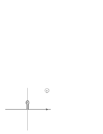
Fig. 1: The contour in the integral over $\nu$ encircling a positive-energy valence state.

The contribution of the Dirac sea levels to observables (e.g. as in (30)) is obtained by carrying numerically the integration over the $v$ variable along the real axis.

We also remark that expressions analogous to (27) hold for any “good” quantum number, i.e. when $[h\left(\nu\right),\lambda_{a}]=0$. For instance, in the Friedberg-Lee-like model, where $\mathchar 8\relax=\sigma$ (no pion field present), the isospin is a good quantum number, and we have, in analogy to (27),

$$I_{3}=-\frac{1}{2}\sum_{k}\intop_{-\infty}^{\infty}\frac{dv}{2\pi i}\frac{(1-i\frac{d\varepsilon_{k}\left(v\right)}{dv})\langle k,\nu|\tau_{3}|k,\nu\rangle}{\nu-i\varepsilon_{k}\left(v\right)},\quad({\rm Freedberg-Lee})$$ (31)

In hedgehog models isospin is not a good quantum number and it has to be restored by a suitable projection method, e.g. by cranking [21, 22].

9 $g_{A}$

Another important quantity is the axial charge of the nucleon, $g_{A}$, evaluated in hedgehog models from the expectation value of the $z$ component of the axial current. In fact, we see that also the space components of current do not depend on the path at $q=0$. Hence $g_{A}$ is path-independent. An explicit expression can be immediately derived from (22), using the method of Ref. [22].

10 Moment of inertia

It is well-known that hedgehog solitons break the spin and isospin, which are restored by a suitable projection method. In the cranking method [21, 22] the basic dynamical quantity is the moment of inertia $\theta$. It is obtained by adiabatically rotating the soliton,

$$\psi(x)\rightarrow e^{-i\tau^{a}\mathchar 10\relax_{a}t}\psi(x),$$ (32)

where $\mathchar 10\relax_{a}$ is the (adiabatically small) velocity of rotation in the isospin space, and $t$ is the time. The moment if inertia is obtained by performing the transformation (32) in the action and then identifying the coefficient of $\mathchar 10\relax^{2}.$ We notice that Eq. (32) is a special case of gauge transformation (5), with the vector potential equal to $A_{a}^{\mu}=(\mathchar 10\relax_{a},0,0,0)$. Therefore we should apply the prescription (9), and then evaluate $\theta$ from the formula $\delta^{2}I/\delta\mathchar 10\relax_{a}\delta\mathchar 10\relax_{b}=\delta^{ab}\theta$. Applying the same techniques as used in the previous sections leads to the following expression for the moment of inertia in models with non-local regulators (Euclidean notation):

$$\theta = -\frac{1}{2}\sum_{k,l}\intop\frac{d\nu}{2\pi}\frac{\langle k,\nu|\left(\tau_{3}-i\tau_{3}\beta r_{0}{\bf\mathchar 8\relax}r-i\beta r{\bf\mathchar 8\relax}r_{0}\tau_{3}\right)|l,\nu\rangle}{i\nu+\varepsilon_{k}(\nu)}\times$$ (33)

$$\times\frac{\langle l,\nu|\left(\tau_{3}-i\tau_{3}\beta r_{0}{\bf\mathchar 8\relax}r-i\beta r{\bf\mathchar 8\relax}r_{0}\tau_{3}\right)|k,\nu\rangle}{i\nu+\varepsilon_{l}(\nu)}$$

$$\ -\sum_{k}\intop\frac{d\nu}{2\pi}\frac{\langle k,\nu|\beta\left(\frac{1}{2}r_{00}{\bf\mathchar 8\relax}r+\tau_{3}r_{0}{\bf\mathchar 8\relax}r_{0}\tau_{3}+\frac{1}{2}r{\bf\mathchar 8\relax}r_{00}\right)|k,\nu\rangle}{i\nu+\varepsilon_{k}(\nu)},$$

where $r_{00}=d^{2}r/d\nu^{2}$. The first term in Eq. (33) is dispersive, it is involves to quark propagators. The second one is the contact term (sea-gull), with one quark propagator looped around. In the local limit Eq. (33) reduces formally to the usual Inglis formula

$$\theta=\frac{1}{2}\sum_{p,h}\frac{|\langle h|\tau_{3}|p\rangle|^{2}}{\varepsilon_{p}-\varepsilon_{h}}.\qquad({\rm local})$$ (34)

In the presence of valence states we proceed as in the case of the baryon number or the soliton energy, and decompose the total moment of inertia into the valence and Dirac sea parts. The valence part is obtained by explicitly occupying the state satisfying Eq. (28).

Notice that $\theta$ in Eq. (33) is path-independent. In fact, it is clear from the derivation that any n-point Green’s function with vanishing momenta on the external current lines does not depend on the choice of the path. This is because the differentiation of the action with respect to the $A$ field at $q=0$ brings down, according to Eq. (12), the factor of $(y-x)_{\mu}$, where $y$ and $x$ are end-points of the line. Then $A$ is set to zero. Obviously, no information of the choice of the path is left.

11 Straight-line paths

The quantities discussed above did not depend on the choice of the path. This is not true for other physical quantities, such as form factors and magnetic moments of baryons, or transverse vector correlators. The simplest choice of the path in the P-exponent is just the straight line, as used in Refs. [9, 10]. One parameterizes $s^{\mu}=x^{\mu}+\alpha(z^{\mu}-x^{\mu})$. Then

$$\intop_{x}^{z}e^{-iq\cdot s}ds_{\mu}=\intop_{0}^{1}d\alpha(z^{\mu}-x^{\mu})e^{-iq\cdot(x+\alpha(z-x))},$$ (35)

and the repetition of the steps of Eq. (7-21) leads to

$$j_{a}^{\mu,{\rm NL}}(q) = -\intop(dp)(dp^{\prime})\intop_{0}^{1}d\alpha\psi^{\dagger}(-p)\times$$ (39)

$$\ \ \ \left[\begin{array}[]{c}r_{\mu}(p+\alpha q)\lambda_{a}\beta{\bf\mathchar 8\relax}(p-p^{\prime}+q)r(p^{\prime})+\\ r(p)\beta{\bf\mathchar 8\relax}(p-p^{\prime}+q)\lambda_{a}r_{\mu}(p^{\prime}-\alpha q)\end{array}\right]\psi(p^{\prime}).$$

In the coordinate representation we can write equivalently

$$j_{a}^{\mu,{\rm NL}}(x)=-\intop_{0}^{1}d\alpha\intop dz\ dx^{\prime}\delta(x-x^{\prime}-\alpha(z-x^{\prime}))\times$$

$$\left[\langle\psi|z\rangle\langle z|r_{\mu}|x^{\prime}\rangle\langle x^{\prime}|\lambda_{a}\beta{\bf\mathchar 8\relax}r|\psi\rangle+\langle\psi|r\beta{\bf\mathchar 8\relax}\lambda_{a}|x^{\prime}\rangle\langle x^{\prime}|r_{\mu}|z\rangle\langle z|\psi\rangle\right].$$ (40)

Expression (39,40) can be used to calculate the non-local contribution to currents.

12 Form factors

Rewriting the general expression (39) for ${\bf\lambda}_{a}=1/N_{c}$ we find the following expression for the non-local contribution to the Fourier-transformed baryon density:

$$\rho^{{\rm NL}}(q)=-\frac{1}{N_{c}}\intop(dp)(dp^{\prime})\intop_{0}^{1}d\alpha\bar{\psi}(-p)\left\{\begin{array}[]{c}r_{0}(p+\alpha q){\bf\mathchar 8\relax}(p-p^{\prime}+q)r(p^{\prime})+\\ r(p){\bf\mathchar 8\relax}(p-p^{\prime}+q)r_{0}(p^{\prime}-\alpha q)\end{array}\right\}\psi(p^{\prime}).$$ (41)

We can now pass to the Breit frame ($q_{0}=0$) and expand Eq. (41) at $\vec{q}=0$. The term quadratic in $\vec{q}$ is related to the non-local contribution to the baryon mean squared radius, which equals to

$$\langle r^{2}\rangle^{{\rm NL}} = \frac{1}{N_{c}}\sum_{i=1}^{3}\intop(dp)(dp^{\prime})\bar{\psi}(-p)\times$$ (45)

$$\ \left[\begin{array}[]{c}\left\{r_{0}(p){\bf\mathchar 8\relax}_{ii}(p-p^{\prime})+r_{0i}(p){\bf\mathchar 8\relax}_{i}(p-p^{\prime})+\frac{1}{3}r_{0ii}(p){\bf\mathchar 8\relax}(p-p^{\prime})\right\}r(p^{\prime})+\\ r(p)\left\{{\bf\mathchar 8\relax}_{ii}(p-p^{\prime})r_{0}(p^{\prime})-{\bf\mathchar 8\relax}_{i}(p-p^{\prime})r_{0i}(p^{\prime})+\frac{1}{3}{\bf\mathchar 8\relax}(p-p^{\prime})r_{0ii}(p^{\prime})\right\}\end{array}\right]\psi(p^{\prime}).$$

The expressions for the isoscalar and isovector magnetic moment involve cranking and are somewhat more complicated. They can be obtained using the methods described above along the lines of Ref. [22].

13 The weak-non-locality limit

It is instructive to have a closer look at Eq. (45). Suppose the soliton has a typical size $R\sim 1/\mathchar 3\relax_{S}$, and the regulator has a momentum scale $\mathchar 3\relax$ above which the momenta are suppressed, e.g. $r(p^{2})=\exp(-p^{2}/\mathchar 3\relax^{2})$. Derivatives with respect to momenta, such as appear in Eqs. (45), bring down a factor of the inverse scale squared, e.g. $r_{\mu}(p^{2})=-2p_{\mu}\exp(-p^{2}/\mathchar 3\relax^{2})/\mathchar 3\relax^{2}$, and similarly for the soliton profile, where $\mathchar 8\relax_{j}(P-P^{\prime})=2(P-P^{\prime})_{j}/\mathchar 3\relax_{S}^{2}$ $\,\mathchar 8\relax^{\prime}(P-P^{\prime})$. In the weak-non-locality limit, i.e. when $\mathchar 3\relax\gg\mathchar 3\relax_{S}$, the terms with derivatives of the regulators are suppressed relative to the terms with derivatives of $\mathchar 8\relax$. For instance, in Eq. (45) we must keep only the terms with $\mathchar 8\relax_{ii}$, and can neglect the remaining pieces. In the coordinate representation this is equivalent to using, instead of (40), the following expression for the non-local current:

$$\ j_{a}^{\mu,{\rm NL}}(x)=-\ \left[\langle\psi|x\rangle\langle x|r_{\mu}\lambda_{a}\beta{\bf\mathchar 8\relax}r|\psi\rangle+\langle\psi|r\beta{\bf\mathchar 8\relax}\lambda_{a}r_{\mu}|x\rangle\langle x|\psi\rangle\right].$$ (46)

One can formally pass from Eq. (40) to Eq. (46) by commuting the $r_{\mu}$ and $|x\rangle\langle x|$ operators, which is allowed in the weak-non-locality limit [3].

For the solitons shown by Bojan Golli $\mathchar 3\relax\sim 1{\rm GeV}$ and $\mathchar 3\relax_{S}\sim.25{\rm GeV}$, hence $\mathchar 3\relax_{S}^{2}/\mathchar 3\relax^{2}\sim 0.06$, hence we seem to be very close to the week-non-locality limit. This is fortunate, since then the observables such as the baryon radius, etc., do not depend strongly on the choice of the path in the P-exponent.

Our research on solitons with non-local regulators is under way and we hope to be able present further exciting results shortly.

References

• [1] D. I. Diakonov and V. Y. Petrov, Nucl. Phys. B 272 (1986) 457
• [2] C. D. Roberts, in QCD Vacuum Structure (World Scientific, Singapore, 1992), p. 114
• [3] G. Ripka, Quarks Bound by Chiral Fields (Oxford University Press, Oxford, 1997)
• [4] J. Praschifka, C. D. Roberts, and R. T. Cahill, Phys. Rev. D 36 (1987) 209
• [5] B. Holdom, J. Terning, and K.Verbeek, Phys. Lett. B 232 (1989) 351
• [6] R. D. Ball, Int. Journ. Mod. Phys. A 5 (1990) 4391
• [7] M. Buballa and S. Krewald, Phys. Lett. B 294 (1992) 19
• [8] R. D. Ball and G. Ripka, in Many Body Physics (Coimbra 1993), edited by C. Fiolhais, M. Fiolhais, C. Sousa, and J. N. Urbano (World Scientific, Singapore, 1993)
• [9] R. D. Bowler and M. C. Birse, Nucl. Phys. A582 (1995) 655
• [10] R. S. Plant and M. C. Birse, Nucl. Phys. A628 (1998) 607
• [11] E. R. Arriola and L. L. Salcedo, Phys. Lett. B450 (1999) 225
• [12] C. Christov, A. Blotz, H. Kim, P. Pobylitsa, T. Watabe, Th. Meissner, E. Ruiz Arriola, and K. Goeke, Prog. Part. Nucl. Phys. 37 (1996) 1
• [13] R. Alkofer, H. Reinhardt, and H. Weigel, Phys. Rep. 265 (1996) 139
• [14] Ö. Kaymakcalan, S. Rajeev, and J. Schechter, Phys. Rev. D 31 (1985) 1109
• [15] E. N. Nikolov, W. Broniowski, C. Christov, G. Ripka, and K. Goeke, Nucl. Phys. A 608 (1996) 411
• [16] V. Dmitrašinović, H.-J. Schulze, R. Tegen, and R. H. Lemmer, Ann. of Phys. (NY) 238 (1995) 332
• [17] W. Florkowski and W. Broniowski, Phys. Lett. B 386 (1996) 62, hep-ph/9605315
• [18] B. Golli, W. Broniowski, and G. Ripka, Phys. Lett. B437 (1998) 24
• [19] J. W. Bos, J. H. Koch, and H. W. C. Naus, Phys. Rev. C 44 (1991) 485
• [20] W. Broniowski, G. Ripka, E. N. Nikolov, and K. Goeke, Z. Phys. A 354 (1996) 421
• [21] G. S. Adkins, C. R. Nappi, and E. Witten, Nucl. Phys. B228 (1983) 552
• [22] T. D. Cohen and W. Broniowski, Phys. Rev. D34 (1986) 3472