The Effect of Shadowing on Initial Conditions, Transverse Energy and Hard Probes in Ultrarelativistic Heavy Ion Collisions

Abstract

The effect of shadowing on the early state of ultrarelativistic heavy ion collisions is investigated along with transverse energy and hard process production, specifically Drell-Yan, $J/\psi$, and $\Upsilon$ production. We choose several parton distributions and parameterizations of nuclear shadowing, as well as the spatial dependence of shadowing, to study the influence of shadowing on relevant observables. Results are presented for Au+Au collisions at $\sqrt{s_{NN}}=200$ GeV and Pb+Pb collisions at $\sqrt{s_{NN}}=5.5$ TeV.

I Introduction

Experiments [1] have shown that the proton and neutron structure functions are modified in the nuclear environment. The modification depends on the parton momentum fraction $x$. For medium $x$, $0.3<x<0.7$, the nuclear parton distributions are depleted relative to those in isolated nucleons. For intermediate $x$, $0.1<x<0.3$, the distributions are enhanced, an effect known as antishadowing. Finally, for small $x$, $x<0.1$, the nuclear depletion returns. We refer to the entire characteristic modification as a function of $x$ as shadowing. To date, most measurements of shadowing have studied charged partons, quarks and antiquarks, through deep-inelastic scattering (DIS), $eA\rightarrow e^{\prime}X$, while the behavior of the nuclear gluon distribution has been inferred from the modifications to the charged partons.

Almost all of these measurements were blind to the position of the nucleons in the nucleus. However, most models of shadowing predict that the structure function modifications should be correlated with the local nuclear density. For example, if shadowing is due to gluon recombination, it should be proportional to the local nuclear density. The only experimental study of spatial dependence of parton distributions relied on dark tracks in emulsion to tag more central collisions [2]. They found evidence of a spatial dependence but could not determine the form.

This paper studies the effect of shadowing and its position dependence in ultrarelativistic Au+Au collisions at a center of mass energy of 200 GeV per nucleon, as will be studied at the Brookhaven Relativistic Heavy Ion Collider (RHIC) and in 5.5 TeV per nucleon Pb+Pb collisions expected at the CERN Large Hadron Collider (LHC). We determine the initial quark, antiquark and gluon production and the first two $E_{T}$ moments of minijet production for two commonly used parton distributions, with three shadowing parameterizations. Following previous calculations, we find the initial energy density and the average energy per particle. We critically examine the concept of fast thermalization in these collisions.

The spatial dependence of shadowing is reflected in particle production as a function of impact parameter, $b$, which may be inferred from the total transverse energy, $E_{T}$, produced in a heavy ion collision [3, 4]. We discuss the relationship between $E_{T}$ and $b$ including both hard and soft contributions. We then consider the effect of shadowing on the production of hard probes such as $J/\psi$, $\Upsilon$, and Drell-Yan dileptons as a function of $b$. These latter calculations complement studies of shadowing in open charm and bottom production [5].

Section 2 discusses the initial state nuclear parton distributions, including shadowing and its spatial dependence. Section 3 then considers minijet production and the effect on initial conditions for further evolution of the system. Section 4 is devoted to the relationship between transverse energy and impact parameter. Section 5 discusses $J/\psi$ and Drell-Yan production and their sensitivity to the nuclear parton distributions. Finally, section 6 gives some conclusions.

II Nuclear Parton Distributions

The nuclear parton densities, $F_{i}^{A}$, are assumed be the product of the nucleon density in the nucleus $\rho_{A}(s)$, the nucleon parton density $f_{i}^{N}(x,Q^{2})$, and a shadowing function $S^{i}(A,x,Q^{2},\vec{r},z)$ where $A$ is the atomic mass number, $x$ is the parton momentum fraction, $Q^{2}$ is the interaction scale, and $\vec{r}$ and $z$ are the transverse and longitudinal location of the parton in position space with $s=\sqrt{|\vec{r}|^{2}+z^{2}}$ so that

$$F_{i}^{A}(x,Q^{2},\vec{r},z) = \rho_{A}(s)S^{i}(A,x,Q^{2},\vec{r},z)f_{i}^{N}(x,Q^{2})\,\,.$$ (1)

In the absence of nuclear modifications, $S^{i}(A,x,Q^{2},\vec{r},z)\equiv 1$. The density of nucleons in the nucleus is given by the Woods-Saxon distribution

$$\rho_{A}(s)=\rho_{0}{1+\omega(s/R_{A})^{2}\over 1+\exp[(s-R_{A})/d]}\,\,.$$ (2)

where the nuclear radius, $R_{A}$, skin thickness, $d$, and oblateness, $\omega$, are determined from low energy electron-nuclear scattering [6]. The central density is determined by the normalization $\int d^{2}rdz\rho_{A}(s)=A$. Results are given for Au+Au collisions at RHIC and Pb+Pb collisions at the LHC with $R_{\rm Au}=6.38$ fm and $R_{\rm Pb}=6.62$ fm respectively.

The densities of parton $i$ in the nucleon are obtained from fits to DIS data. These fits are necessary because the distributions at the initial scale $Q_{0}$ are nonperturbative. However, the parameterizations of $f_{i}^{N}$ are only reliable where measurements exist. The continually improving DIS data from HERA [7] shows that uncertainties still exist at small $x$. Therefore, we consider two different parton distribution sets. Both are chosen because they are leading order, LO, sets which are more consistent with a leading order calculation. They also have a relatively low initial scale. The GRV 94 LO [8] distributions have a lower scale, $Q_{0}=0.63$ GeV, than the MRST LO [9] central gluon distribution with $Q_{0}=1$ GeV. Figure 1 compares the valence, $q_{V}=u_{V}+d_{V}$, sea quark, $q_{S}=2(\overline{u}+\overline{d}+\overline{s})$, and the gluon, $g$ distributions at $Q^{2}=4$ GeV² of the two sets. In the low $x$ region probed by the LHC the valence and sea quark distributions in both sets are similar. However, the MRST LO gluon distribution is less than half as large as the GRV 94 LO gluon distribution. As we show in the next section, the gluons dominate particle production at the LHC. Thus the low $x$ gluon density will significantly affect the initial conditions obtained for these high energies. At $x\sim 0.01$ the parton densities are well known so that the two sets are similar and the choice of the proton parton distributions do not strongly influence the initial conditions at RHIC.

Shadowing is an area of intense study with numerous models available in the literature[1]. However, none of the models can satisfactorily explain the behavior of the nuclear parton distributions over the entire $x$ and $Q^{2}$ range. Therefore, we choose to use parameterizations of shadowing based on data. We use three different fits, all based on nuclear DIS data. As in DIS with protons, the nuclear gluon distribution is not directly measured and can only be inferred from conservation rules. The first parameterization, $S_{1}(A,x)$, treats quarks, antiquarks, and gluons identically without $Q^{2}$ evolution [10]. The other two evolve with $Q^{2}$ and conserve baryon number and total momentum. The $S_{2}^{i}(A,x,Q^{2})$ parameterization, starting from the Duke-Owens parton densities [11], modifies the valence quarks, sea quarks and gluons separately and includes $Q^{2}$ evolution for $Q_{0}=2<Q<10$ GeV [12]. The third parameterization, $S_{3}^{i}(A,x,Q^{2})$, is based on the GRV LO [13] parton densities. Each parton type is evolved separately above $Q_{0}=1.5$ GeV [14, 15]. The initial gluon distribution in $S_{3}$ shows significant antishadowing for $0.1<x<0.3$ while the sea quark distributions are shadowed. In contrast, $S_{2}$ has less gluon antishadowing and essentially no sea quark effect in the same $x$ region. Since $S_{3}$ includes the most recent nuclear DIS data, it should perhaps be favored. Figure 2 compares $S_{1}$, $S_{2}$ and $S_{3}$ for $Q=Q_{0}$ and $Q=10$ GeV.

The remaining ingredient is the spatial dependence of the shadowing. Unfortunately, there is little relevant data. Fermilab experiment E745 studied the spatial distribution of nuclear structure functions with $\nu N$ interactions in emulsion. The presence of one or more dark tracks from slow protons is used to infer a more central interaction[2]. For events with no dark tracks, no shadowing is observed while for events with dark tracks, shadowing is enhanced over spatially independent measurements from other experiments. Unfortunately, this data is too limited to be used in a fit of the spatial dependence.

Most models of shadowing predict that the nuclear parton densities should depend on the interaction point within the nucleus. In one model, at high parton density gluons and sea quarks from one nucleon can interact with partons in an adjacent nucleon[16] so that shadowing is proportional to the local density, Eq. (2) [3, 5]. Then

$$S^{i}_{\rm WS}=S^{i}(A,x,Q^{2},\vec{r},z) = 1+N_{\rm WS}[S^{i}(A,x,Q^{2})-1]\frac{\rho_{A}(s)}{\rho_{0}}\,\,,$$ (3)

where $N_{\rm WS}$ is chosen so that $(1/A)\int d^{2}rdz\rho_{A}(s)S^{i}_{\rm WS}=S^{i}$. At large distances, $s\gg R_{A}$, the nucleons behave as free particles while in the center of the nucleus, the modifications are larger than the average value $S^{i}$.

In another approach, shadowing stems from multiple interactions by an incident parton[17]. Parton-parton interactions are spread longitudinally over a distance known as the coherence length, $l_{c}=1/2mx$, where $m$ is the nucleon mass[18]. For $x<0.016$, $l_{c}$ is greater than any nuclear radius and the interaction of the incoming parton is delocalized over the entire trajectory. The incident parton interacts coherently with all of the target partons along this interaction length. At large $x$, $l_{c}\ll R_{A}$ and shadowing is proportional to the local density at the interaction point, while for small $x$, it depends on the density integrated over the incident parton trajectory. Both formulations reproduce the spatially independent shadowing data quite well. Unfortunately, the available data[2] is inadequate to test these theories.

Because of the difficulty of matching the shadowing at large and small $x$ while maintaining baryon number and momentum conservation, we do not include the multiple scattering model explicitly in our calculations. However, we do consider the small $x$ and large $x$ limits separately. Equation (3) corresponds to the large $x$ limit. In the small $x$ regime, the spatial dependence may be parameterized

$$S^{i}_{\rho}(A,x,Q^{2},\vec{r},z)=1+N_{\rho}(S^{i}(A,x,Q^{2})-1)\int dz\rho_{A}(\vec{r},z)\,\,.$$ (4)

The integral over $z$ includes the material traversed by the incident nucleon. The normalization requires $(1/A)\int d^{2}rdz\rho_{A}(s)S^{i}_{\rho}=S^{i}$. We find $N_{\rho}>N_{\rm WS}$.

There are a number of difficulties with the coherent-interaction picture. While traversing the formation length, both the incident and the produced partons will undergo multiple interactions, which will reduce the effective coherence length, analogous to the Landau-Pomeranchuk-Migdal effect[19]. Also, the picture of a single incident parton interacting with a static nucleus is inappropriate in heavy ion collisions since the parton density rises rapidly as many interactions occur simultaneously. A step-by-step calculation cannot solve this problem because non-local depictions of heavy ion collisions are inevitably Lorentz frame dependent [20]. Finally, in a model where the parton densities are spread out over an $x$-dependent distance, baryon number is not locally conserved.

We previously considered a variant, $S_{\rm R}^{i}$, where shadowing is proportional to the thickness of a spherical nucleus at the collision point[3],

$$S^{i}_{\rm R}(A,x,Q^{2},\vec{r},z)=\left\{\begin{array}[]{ll}1+N_{\rm R}(S^{i}(A,x,Q^{2})-1)\sqrt{1-(|\vec{r}|/R_{A})^{2}}&\mbox{$r\leq R_{A}$}\\ 1&\mbox{$r>R_{A}$}\end{array}\right.\,\,.$$ (7)

The normalization, $N_{\rm R}$, obtained after averaging over $\rho_{A}(s)$, is similar to $N_{\rho}$. This model suffers from a discontinuous derivative at $r=R_{A}$ with no shadowing predicted for $r>R_{A}$, but is otherwise fairly similar to $S_{\rho}$.

Figure 3 compares the radial dependence of $S_{\rm WS}$, $S_{\rho}$, and $S_{\rm R}$ for $S^{i}(A,x,Q^{2})=0.7$. For the comparison, $S_{\rm WS}$ is evaluated at $z=0$. The $S_{\rho}$ and $S_{\rm R}$ results are very similar except near the nuclear surface where they differ by $\approx 10$%. Later we compare calculations of the first $E_{T}$ moment with $S_{\rm WS}$ and $S_{\rho}$ and show that the two results are very similar. Calculations using $S_{\rho}$ and $S_{\rm R}$ would be in closer agreement, effectively indistinguishable.

Other mechanisms such as nuclear binding have also been suggested as possible explanations of shadowing[21]. These calculations can explain only a small fraction of the observed effect[22], at least for $x>0.1$. However, many of these models would also predict some spatial dependence.

Given the difficulties of matching spatial dependencies for different $x$ and $A$ while preserving baryon and momentum conservation in the multiple interaction model, we focus our calculations on the local density model, and perform most of our calculations using $S_{\rm WS}$. However, as we will show, the calculations are relatively insensitive to the exact parameterization suggesting that heavy ion collision studies will not distinguish between different models.

For simplicity, we will refer to homogeneous (without spatial dependence) and inhomogeneous (position dependent) shadowing.

III Initial Conditions in $A+A$ Collisions

At RHIC and LHC perturbative QCD processes are expected to be an important component of the total particle production. At early times, $\tau_{i}\sim 1/p_{T}\leq 1/p_{0}\sim 0.1$ fm for $p_{0}\sim 2$ GeV, semihard production of low $p_{T}$ minijets will set the stage for further evolution [23]. Copious minijet production, especially gluonic minijets, in the initial $NN$ collisions has been suggested as a mechanism for rapid thermalization, particularly at the LHC. We critically examine this idea, with special attention to the effects of shadowing on these expectations.

Minijet production is calculated from the jet cross section for $p_{T}>p_{0}$. At leading order the rapidity, $y$, distribution of a parton flavor $f$ produced in the parton subprocess $ij\rightarrow kl$ in $AB$ collisions is [24]

$$\frac{d\sigma^{f}(p_{0})}{d^{2}bd^{2}rdy} = K_{\rm jet}\int dp_{T}^{2}dy_{2}dzdz^{\prime}\sum_{{ij=}\atop{\langle kl\rangle}}x_{1}F_{i}^{A}(x_{1},p_{T}^{2},\vec{r},z)x_{2}F_{j}^{B}(x_{2},p_{T}^{2},\vec{b}-\vec{r},z^{\prime})$$ (9)

$$\mbox{}\times\frac{1}{1+\delta_{kl}}\left[\delta_{fk}{d\hat{\sigma}\over d\hat{t}}^{ij\rightarrow kl}(\hat{t},\hat{u})+\delta_{fl}{d\hat{\sigma}\over d\hat{t}}^{ij\rightarrow kl}(\hat{u},\hat{t})\right]\,\,,$$

where $\hat{t}=-p_{T}^{2}(1+e^{-(y-y_{2})})$ and $\hat{u}=-p_{T}^{2}(1+e^{(y-y_{2})})$. The limits of integration on $p_{T}^{2}$ and $y_{2}$ are $p_{0}^{2}<p_{T}^{2}<s_{NN}/(4\cosh^{2}y)$ and $\ln(r_{p_{T}}-e^{-y})\leq y_{2}\leq\ln(r_{p_{T}}-e^{y})$ where $|y|\leq\ln(r_{p_{0}}+\sqrt{r_{p_{0}}^{2}-1})$, $r_{p_{T}}=\sqrt{s_{NN}}/p_{T}$ and $r_{p_{0}}=\sqrt{s_{NN}}/2p_{0}$. The sum over initial states includes all combinations of two parton species with three flavors while the final state includes all pairs without a mutual exchange and four flavors (including charm) so that $\alpha_{s}(p_{T})$ is calculated at one loop with four flavors. The factor $1/(1+\delta_{kl})$ accounts for the identical particles in the final state. The factor $K_{\rm jet}$ in Eq. (9) is the ratio of the NLO to LO jet cross sections and indicates the size of the NLO corrections. Previous analysis of high $p_{T}$ jets predicted $K_{\rm jet}\approx 1.5$ at LHC energies [25]. A more recent NLO calculation of minijet production found $K_{\rm jet}\approx 2$ at both RHIC and LHC [26]. Assuming $K_{\rm jet}=1$, as in Ref. [24], gives a conservative lower limit on minijet production. The cutoff $p_{0}$, represents the lowest $p_{T}$ scale at which perturbative QCD is valid. There is some uncertainty in the exact value of $p_{0}$ which can be constrained by soft physics [27]. However, 2 GeV should be a safe value for heavy ion collisions, especially at the LHC[24]. The effects of different choices for $p_{0}$ will be discussed later.

The parton densities are evaluated at scale $p_{T}$, with $x$ values at as low as $x_{1,2}\sim 2p_{0}/\sqrt{s_{NN}}\sim 7\times 10^{-4}$ at $y=y_{2}=0$ in Pb+Pb collisions at 5.5 TeV/nucleon. At higher rapidities, $x_{1}$ or $x_{2}$ can be even smaller. Thus the small $x$ behavior of the parton densities strongly influences the initial conditions of the minijet system.

The resulting minijet rapidity distributions are shown in Figs. 4-7 for the two sets of parton distributions at the LHC and RHIC both without shadowing and with homogeneous shadowing. Shadowing can reduce the number of produced partons by up to a factor of two at the LHC, depending on the parameterization and the parton type. The smallest effect is observed with the newer $S_{3}$ parameterization. At the lower RHIC energy, $x_{1,2}\sim 0.02$, and shadowing is smaller, as is shown in Fig. 2. Due to the strong antishadowing, gluons are actually enhanced with $S_{3}$.

Since each collision has two final state partons, the total number of partons of flavor $f$ at impact parameter $b$ is

$$\overline{N}^{f}(b,p_{0})=2\,\frac{d\sigma^{f}(p_{0})}{d^{2}b}\,\,$$ (10)

where $d\sigma^{f}(p_{0})/d^{2}b$ is the integral of Eq. (9) over $d^{2}r$ and $dy$ normalized so that

$$\int\frac{d\sigma^{f}(p_{0})}{d^{2}bdy}dy=2\frac{d\sigma^{f}(p_{0})}{d^{2}b}$$ (11)

because there are two final-state partons in each collision. The total hard scattering cross section as a function of impact parameter is the sum over all parton flavors so that

$$2\sum_{f}\frac{d\sigma^{f}(p_{0})}{d^{2}b}=2\frac{d\sigma(p_{0})}{d^{2}b}\equiv\sigma^{H}(b,p_{0})\,\,.$$ (12)

When $S=1$ or $S\equiv S^{i}(A,x,Q^{2})$ the spatial dependence factorizes, the per nucleon cross section is independent of $b$, and the total cross section scales with the nuclear overlap function, $T_{AB}(b)$, [28]. The overlap function is the convolution of the nuclear density distributions [6]

$$T_{AB}(b)=\int d^{2}\vec{r}T_{A}(\vec{r})T_{B}(\vec{b}-\vec{r})$$ (13)

with the nuclear thickness function $T_{A}(\vec{r})=\int dz\rho_{A}(z,\vec{r})$. For $AA$ collisions, $T_{AA}(0)\approx A^{2}/(\pi R_{A}^{2})\propto A^{4/3}$. The transverse area of the system and the initial volume at $b=0$ are

$$A_{T} = \pi R_{A}^{2}$$ (14)

$$V_{i} = A_{T}\Delta y\tau_{i}=A_{T}\Delta y/p_{0}\,\,,$$ (15)

where $\tau_{i}=1/p_{0}$ and $\Delta y$ is the rapidity range.

Parton production saturates when the transverse area occupied by the partons is larger than the total transverse area available. The total number of partons produced in the collision is the sum over flavors,

$$\overline{N}^{H}(b)=\sum_{f}\overline{N}^{f}(b,p_{0})$$ (16)

In a $b=0$ collision, the partons occupy a transverse area $\pi\overline{N}^{H}(0)/p_{0}^{2}$. Saturation occurs when the area occupied by partons is equivalent to the transverse area of the target in a symmetric heavy ion collision at $b=0$, $\overline{N}^{H}(0)>R_{A}^{2}p_{0}^{2}$. In Pb + Pb collisions $T_{AA}(0)=30.4$/mb and saturation occurs if the hard cross section is greater than 74 ($p_{0}$/2 GeV)² mb. At the LHC, gluons alone are sufficient to saturate the transverse area, even with shadowing. For Au + Au collisions at RHIC, the hard cross section must be more than 71 ($p_{0}$/2 GeV)² mb. This condition is not satisfied at RHIC, unless $p_{0}$ is lowered to $\sim 1$ GeV[27]. However, 1 GeV is close to if not within the nonperturbative regime, suggesting that soft physics still dominates particle production at RHIC.

These conclusions depend on the small $x$ behavior of the gluon distribution, the factor $K_{\rm jet}$, the cutoff $p_{0}$, and the shadowing parameterization. Transverse saturation does not occur at the LHC when the MRST LO set is used if $K_{\rm jet}=1$. An empirical $K_{\rm jet}$ may be obtained by comparing model calculations to data, giving some freedom in the value of $K_{\rm jet}$ for different parton distributions. However, less variation is allowed in the theoretical values of $K_{\rm jet}$ obtained from the ratio of the NLO and LO cross sections. The theoretical $K_{\rm jet}$ does, however, tends to rise as $p_{T}$ decreases, rendering calculations with $p_{0}<2$ GeV less reliable.

Transverse saturation at $p_{0}=2$ GeV implies that the minijet cross section exceeds the inelastic $pp$ cross section, violating unitarity. This is especially a problem for the GRV 94 LO distributions because of the high gluon density at low $x$. At very low $x$ then, the proton is like a black disk and instead of further splitting to increase the density of partons, the partons begin to recombine, acting to lower the density below that without recombination. Therefore at very low $x$, the density of partons should not increase without bound but begin to saturate. This recombination corresponds to one picture of shadowing in the proton [16]. A recent HERA measurement of the derivative of the structure function $F_{2}$ found that at low $x$ and $Q^{2}$, $dF_{2}/d\ln Q^{2}$ no longer increases, in contrast to the GRV 94 parton densities which continue to increase over the range of their validity [29]. The newer MRST distributions have been tuned to fit this behavior for $Q^{2}>1$ GeV². This data implies that the unitarity violation in $pp$ interactions is likely an artifact of the free proton parton densities.

The magnitude of the problem can be gauged by calculating the number of collisions suffered by incoming partons. If, on average, a parton collides more than once while crossing the nucleus, unitarity violation is a serious problem. The higher the incoming parton $x_{1}$, the more low $x_{2}$ target partons are available for it to interact with, the larger the interaction cross section, and the subsequent number of collisions. The minimum $x_{2}$ depends on $p_{0}$ and $\sqrt{s_{NN}}$. Since the gluon interaction cross sections are larger than those of quarks, we focus on incoming gluons with $x=0.1$. The average number of collisions experienced by such an initial gluon at the LHC is shown in Fig. 8(a) and (b) for GRV 94 LO and MRST LO distributions respectively. The scattering cross section has been multiplied by the nuclear profile function $T_{A}(b)$ to give the number of collisions. A gluon can suffer up to an average of 5 hard scatterings in central collisions with GRV 94 LO and $S=1$. It experiences less than one collision in the target when $b>5-6$ fm. Shadowing reduces the severity of the problem by decreasing the number of scatterings by $\approx 30$%. On the other hand, $u$ and $\overline{u}$ quarks with $x=0.1$ typically scatter once or less in the target, even without shadowing. With the MRST LO distributions, the unitarity violation is less severe, with $1.4-2$ scatterings per central collision for gluons and 0.5 $u$ or $\overline{u}$ collisions per central event.

Therefore we might expect that to satisfy unitarity, transverse saturation cannot be used as a criteria for determining $p_{0}$ and early equilibration by minijet production is unlikely in reality. At the lower RHIC energy, unitarity is always satisfied with incoming partons experiencing an average of less than one collision. Figure 8(c) and (d) shows this for the gluon. The $q$ and $\overline{q}$ results are considerably smaller.

The quark rapidity distribution, $d\sigma^{q}/dy$ is indicative of baryon stopping due to hard processes. As Tables I-IV and Figs. 4-7 show, at LHC energies, the GRV 94 LO parton distributions predict considerably larger stopping than MRST LO. These homogeneous shadowing cross sections can be converted to $dN/dy$ at any impact parameter by multiplying by $T_{AB}(b)$. Although both parton distributions predict similar baryon densities at mid-rapidity, GRV 94 LO predicts about twice as many baryons at large rapidity than MRST LO. Because of the unitarity problems and the high gluon density at low $x$, at LHC the final state baryon number, $\int dy(dq/dy-d\overline{q}/dy)/3$, exceeds the baryon number of the two incoming nuclei. This is a clear result of the unitarity violation. Previous works[24] noted this but suggested that the problem is reduced if only central rapities are considered, typically $|y|<0.5$. A better solution would include a more complete treatment of multiple scattering. However, such a calculation involves even more uncertainties. At RHIC energies, the cross sections are lower, and baryon conservation is not an issue. The two sets of parton distributions make similar predictions, with MRST LO finding a somewhat higher baryon density at mid-rapidity.

We present calculations covering the entire range of rapidities, even though at the LHC, at large rapidity, $|y|>5$, either $x_{1}$ or $x_{2}$ is outside the stated validity range of the parton distributions. This range problem could affect calculations at all $y$ since a parton density that satisfies the unitarity bound at $p_{0}$ will be different at all rapidities since more of the low $x$ rise will be subsumed into higher $x$ values to maintain momentum conservation.

We would like to determine the effects of shadowing on the quantities such as the energy density which are important for our understanding of the initial conditions. The initial energy density is directly related to the cross section times first $E_{T}$ moment of each flavor, $\sigma^{f}(p_{0})\langle E_{T}^{f}\rangle$, which is calculated within a specific acceptance. A crude approximation of the acceptance is

$$\epsilon(y)=\left\{\begin{array}[]{ll}1&\mbox{if $|y|\leq y_{\rm max}$}\\ 0&\mbox{otherwise}\end{array}\right.$$ (19)

where $y_{\rm max}$ is the highest measurable rapidity. At leading order, the parton pairs are produced back-to-back. The $E_{T}$ distribution of each flavor as a function of impact parameter is [24]

$$\frac{d\sigma^{f}(p_{0})}{dE^{f}_{T}d^{2}bd^{2}r} = \frac{K_{\rm jet}}{2}\int dp_{T}^{2}dy_{2}dydzdz^{\prime}\sum_{{ij=}\atop{\langle kl\rangle}}x_{1}F_{i}^{A}(x_{1},p_{T}^{2},\vec{r},z)x_{2}F_{j}^{B}(x_{2},p_{T}^{2},\vec{b}-\vec{r},z^{\prime})$$ (22)

$$\mbox{}\times\frac{1}{1+\delta_{kl}}\left\{{d\hat{\sigma}\over d\hat{t}}^{ij\rightarrow kl}(\hat{t},\hat{u})\delta(E^{f}_{T}-\left[\delta_{fk}\epsilon(y)+\delta_{fl}\epsilon(y_{2})\right]p_{T})\right.$$

$$\mbox{}\left.+{d\hat{\sigma}\over d\hat{t}}^{ij\rightarrow kl}(\hat{u},\hat{t})\delta(E^{f}_{T}-\left[\delta_{fl}\epsilon(y)+\delta_{fk}\epsilon(y_{2})\right]p_{T})\right\}\,\,.$$

Equation (22) is valid for $E_{T}>E_{T\,{\rm min}}$ where the $E_{T\,{\rm min}}$ required in $pp$ collisions is such that $\sigma^{H}\leq\sigma_{\rm inelastic}$ for $E_{T\,{\rm min}}\approx 2$ GeV at 5.5 TeV and 1 GeV at 200 GeV [26]. Therefore, integration over $d^{2}r$ and $E_{T}>E_{T\,{\rm min}}$ reduces Eq. (22) to the total hard cross section as a function of impact parameter

$$\sum_{f}\int d^{2}r\int_{E_{T}\,{\rm min}}^{\infty}\frac{d\sigma^{f}(p_{0})}{d^{2}bd^{2}rdE_{T}^{f}}dE_{T}^{f}=2\frac{d\sigma(p_{0})}{d^{2}b}\equiv\sigma^{H}(b,p_{0})\,\,\,.$$ (23)

The last definition in Eq. (23) holds for $E_{T\,{\rm min}}=p_{0}$, as in Eq. (12).

The first $E_{T}$ moment is obtained by weighting Eq. (22) with $E^{f}_{T}$ and integrating over $E^{f}_{T}$; we neglect particle masses so that $E^{f}_{T}=p_{T}$,

$$\frac{d\sigma^{f}(p_{0})\langle E_{T}^{f}\rangle}{d^{2}bd^{2}r} = K_{\rm jet}\int dp_{T}^{2}dy_{2}dydzdz^{\prime}\sum_{{ij=}\atop{\langle kl\rangle}}x_{1}F_{i}^{A}(x_{1},p_{T}^{2},\vec{r},z)x_{2}F_{j}^{B}(x_{2},p_{T}^{2},\vec{b}-\vec{r},z^{\prime})$$ (25)

$$\mbox{}\times\frac{\epsilon(y)p_{T}}{1+\delta_{kl}}\left[\delta_{fk}{d\hat{\sigma}\over d\hat{t}}^{ij\rightarrow kl}(\hat{t},\hat{u})+\delta_{fl}{d\hat{\sigma}\over d\hat{t}}^{ij\rightarrow kl}(\hat{u},\hat{t})\right]\,\,.$$

The first $E_{T}$ moment is given as a function of rapidity in Figs. 9-12 both with and without impact parameter averaged shadowing for the GRV 94 LO and MRST LO parton densities at LHC and RHIC. The average transverse energy given to a particular parton species in a central $AB$ collision is then

$$\overline{E}_{T}^{f}(b,p_{0})=\frac{d\sigma^{f}(p_{0})\langle E_{T}^{f}\rangle}{d^{2}b}$$ (26)

where $d\sigma^{f}(p_{0})\langle E_{T}^{f}\rangle/d^{2}b$ is the integral of Eq. (25) over $d^{2}r$. If the nuclear structure functions are homogeneous, then the spatial effects factorize and $\overline{E}_{T}^{f}(b,p_{0})$ is proportional to $T_{AB}(b)$. The first $E_{T}$ moment is proportional to the energy density, as we discuss shortly.

The second moment of each flavor is calculated similarly,

$$\frac{d\sigma^{f}(p_{0})\langle E_{T}^{2\,f}\rangle}{d^{2}bd^{2}r} = K_{\rm jet}\int dp_{T}^{2}dy_{2}dydzdz^{\prime}\sum_{{ij=}\atop{\langle kl\rangle}}x_{1}F_{i}^{A}(x_{1},p_{T}^{2},\vec{r},z)x_{2}F_{j}^{B}(x_{2},p_{T}^{2},\vec{b}-\vec{r},z^{\prime})$$ (29)

$$\mbox{}\times\frac{p_{T}^{2}}{1+\delta_{kl}}\left\{\left[\delta_{fk}{d\hat{\sigma}\over d\hat{t}}^{ij\rightarrow kl}(\hat{t},\hat{u})+\delta_{fl}{d\hat{\sigma}\over d\hat{t}}^{ij\rightarrow kl}(\hat{u},\hat{t})\right]\epsilon(y)\right.$$

$$\mbox{}+\left.\left[{d\hat{\sigma}\over d\hat{t}}^{ij\rightarrow ff}(\hat{t},\hat{u})+{d\hat{\sigma}\over d\hat{t}}^{ij\rightarrow ff}(\hat{u},\hat{t})\right]\epsilon(y)\epsilon(y_{2})\right\}\,\,.$$

The terms proportional to $\epsilon(y)\epsilon(y_{2})$ in Eq. (29) correspond to only those processes that contain identical particles in the final state: $qq\rightarrow qq$, $\overline{q}\overline{q}\rightarrow\overline{q}\overline{q}$, $q\overline{q}\rightarrow gg$ and $gg\rightarrow gg$. These terms are negligible for $f=q$ and $\overline{q}$ but large for $f=g$. Indeed, $ff=gg$ in Eq. (29) contributes $\approx 30$% of the total second $E_{T}$ moment of the gluon. The second moment is

$$\overline{E^{2\ f}_{T}}(b,p_{0})=\frac{d\sigma^{f}(p_{0})\langle E_{T}^{2\,f}\rangle}{d^{2}b}\,\,$$ (30)

where $d\sigma^{f}(p_{0})\langle E_{T}^{2\,f}\rangle/d^{2}b$ is the integral of Eq. (29) over $d^{2}r$. For homogeneous structure functions, factorization again occurs and $\overline{E^{2\ f}_{T}}(b,p_{0})$ scales with $T_{AB}(b)$.

We now discuss the results characteristic to specific detectors. We will concentrate on the coverage around midrapidity, thereby excluding some detector subsystems from our consideration. In all cases we assume full azimuthal coverage. At the LHC, there will be two detectors taking data with heavy ion beams, CMS [32], optimized for $pp$ studies but with a broad rapidity coverage, $y_{\rm max}=2.4$, and ALICE [33], a dedicated heavy ion experiment with central rapidity coverage up to $y_{\rm max}=1$. We do not include the ALICE forward muon spectrometer. The heaviest ions accelerated will be lead. STAR [34] and PHENIX [35] are the two large heavy ion experiments at RHIC, a dedicated heavy ion collider that will accelerate ions through gold. STAR has the larger acceptance at central rapidities, $y_{\rm max}=0.9$ for the electromagnetic calorimeter, while the central electron arms of PHENIX only cover up to $y_{\rm max}=0.35$. The PHENIX muon arms will cover more forward rapidities but will not increase the coverage at midrapidity except for high mass lepton pairs such as those from $\Upsilon$ decay. The cross sections per nucleon pair and the first and second $E_{T}$ moments with and without homogeneous shadowing are given in Tables I and II in the given CMS and ALICE rapidity ranges respectively. At this energy, shadowing can reduce the parton yield and the $E_{T}$ moments by up to a factor of two. The corresponding results from RHIC are presented in Tables III and IV for STAR and PHENIX. The effect of shadowing is much smaller at RHIC than at the LHC. In fact, with $S_{3}$, gluon antishadowing can increase the yield relative to $S=1$. Recall that the cross sections and moments are all calculated with $K_{\rm jet}=1$ and another choice would scale the results correspondingly.

The effect of the inhomogeneous shadowing is shown for the first $E_{T}$ moment calculated with the GRV 94 LO parton densities in Figs. 13 and 14 for CMS and STAR. The ALICE and PHENIX ratios are similar to those shown here. The ratios of the other moments do not differ greatly from the first moment. The impact parameter dependence is calculated using Eqs. (3) and (4). When $x$ lies in the shadowing region, central collisions are more shadowed than the average. In the antishadowing region, central collisions are more antishadowed than the average. When $b\sim R_{A}$, the homogeneous and inhomogeneous shadowing are approximately equal, as might be expected from an inspection of Eqs. (3) and (4). When $b\sim 2R_{A}$, the shadowing or antishadowing is significantly reduced. As $b$ further increases, the approach to $S=1$ is asymptotic. With $S_{\rho}$, Eq. (4), the central shadowing is somewhat stronger than with $S_{\rm WS}$ and the strength of the shadowing decreases more rapidly when $b>R_{A}$. At $b\sim 2R_{A}$, the ratio with $S_{\rho}$ is 5% higher than with $S_{\rm WS}$. A calculation with $S_{\rm R}$, Eq. (7), would have somewhat stronger shadowing than $S_{\rho}$. Since the inhomogeneous calculations agree within a few percent, the exact dependence cannot be experimentally distinguished; only the presence of inhomogeneity can be detected. This conclusion applies to a wide variety of observables[3]. Because the differences are small, we use only the $S_{\rm WS}$ parameterization in the remainder of this work.

The figures show the ratio of the first $E_{T}$ moment with shadowing included relative to $S=1$ as a function of impact parameter for $q+\overline{q}$, $g$, and the total, $q+\overline{q}+g$. At the LHC, quarks and antiquarks are $\approx 10$% of the total minijet production for the GRV 94 LO parton densities and $\approx 17$% with the MRST LO densities when $S=1$. The overall $q+\overline{q}$ contribution decreases 1-2% when shadowing is included. At RHIC, the $q+\overline{q}$ fraction is $\approx 19$% with the GRV 94 LO densities and $\approx 23$% with the MRST LO set. There is again only an $\approx 1$% variation in the fraction with shadowing included. The ratios in the given rapidity intervals with homogeneous shadowing are given by the horizontal lines on Figs. 13 and 14 and correspond to the ratio of the moments in Figs. 9 and 11 integrated over the same rapidity intervals. At the LHC, the ratios are nearly the same for the gluon fraction and the total because gluons dominate minijet production. At RHIC energies, since the $q+\overline{q}$ contribution is a larger fraction of the total, the difference between the $g$ ratio and the total, shown in Figs. 13 and 14, is visible, particularly for $S_{3}$ which is shadowed for $q+\overline{q}$ and antishadowed for the gluons. The total remains antishadowed, but less than for gluons alone.

The homogeneous shadowing ratios can also be determined for the zeroth moment, particle number, and the second moment of of the $E_{T}$ distribution, from Tables I-IV. The second $E_{T}$ moment has a slightly smaller $q+\overline{q}$ fraction due to the term in Eq. (29) proportional to $\epsilon(y)\epsilon(y_{2})$ which arises from identical particles in the final state. The dominant contribution to this term is $gg\rightarrow gg$, enhancing the overall gluon contribution.

We now show how the initial conditions for further evolution of the system are impacted by shadowing. The initial energy density of each parton species is the ratio of the first $E_{T}$ moment to the initial volume

$$\epsilon_{i}^{f}(b,p_{0})=\frac{\overline{E}_{T}^{f}(b,p_{0})}{V_{i}}\,\,.$$ (31)

The total initial energy density is the sum over all species, $\epsilon_{i}=\sum_{f}\epsilon_{i}^{f}$. The initial number densities are likewise

$$n_{i}^{f}(b,p_{0})=\frac{\overline{N}^{f}(b,p_{0})}{V_{i}}$$ (32)

and $n_{i}=\sum_{f}n_{i}^{f}$. The energy and number densities are given in Tables V-VIII, both for gluons only and the total minijet yield. Results are shown for both homogeneous and inhomogeneous shadowing at $b=0$ where the volume is most clearly defined. Since shadowing is stronger in central collisions, the energy density and multiplicity are reduced with $S^{i}_{\rm WS}$ relative to the homogeneous case. (See Figs. 13 and 14 for the impact parameter dependence of $\overline{E}_{T}^{f}$.) At the LHC, inhomogeneous shadowing reduces the energy density by $\approx 3$-8% at $b=0$. At RHIC, the difference is smaller and the energy density may even rise marginally at $b=0$ with the $S_{3}$ parameterization. The average energy per particle for a given species is $\epsilon_{i}^{f}/n_{i}^{f}\sim 3$ GeV, somewhat larger than $p_{0}$, as can be expected since $\overline{E}_{T}^{f}$ reflects the average $p_{T}$ within the rapidity range.

These densities can be compared to those obtained for an ideal gas in thermal equilibrium. An ideal gas has energy density $\epsilon_{\rm th}=3aT_{\rm th}^{4}$ and entropy density $s_{\rm th}=4aT_{\rm th}^{3}=3.6n_{\rm th}$ where $a=16\pi^{2}/90$ for a gluon gas and $a=47.5\pi^{2}/90$ for a three flavor quark-gluon plasma. The initial equilibrium temperatures of such gases are then $T_{\rm th}=(\epsilon_{\rm th}/3a)^{1/4}$ and the ideal energy per particle is

$$\frac{\epsilon_{\rm th}}{n_{\rm th}}=2.7\,T_{\rm th}\,\,.$$ (33)

We use the results of Tables V-VIII with the assumption that $\epsilon_{i}=\epsilon_{\rm th}$. When $S=1$, $T_{\rm th}\approx 1.07$ GeV for gluons only and $\approx 840$ MeV for a quark-gluon plasma at the LHC with the GRV 94 LO distributions and $p_{0}=2$ GeV. Using the MRST LO results with $p_{0}=2$ GeV yields $T_{\rm th}\approx 860$ MeV and 680 MeV respectively. The calculated initial quark-gluon plasma temperature is lower than that for gluons because, even though $\epsilon_{i}$ is larger for the sum of all species, the larger number of available degrees of freedom reduces the temperature. Shadowing reduces $T_{\rm th}$ by 10-17% for the gluons and 10-15% for the total with the largest effect due to $S_{1}$ and the smallest from $S_{3}$ with its antishadowing. At RHIC, the equivalent temperatures extracted with $p_{0}=2$ GeV are smaller, 410 MeV for gluons and 330 MeV for a quark-gluon plasma with $S=1$. The reduction due to shadowing is 5% or less—in fact a slight enhancement is possible because of the antishadowing in $S_{3}$. The temperatures are virtually independent of the parton distributions at this energy since the two sets are very similar in the $x$ range of RHIC. The temperatures estimated for RHIC are lower than those obtained elsewhere. This difference will be discussed in the next section.

These equivalent equilibrium temperatures are only approximate because they depend on the rapidity range over which $T_{\rm th}$ is calculated. The extracted temperature rises as the rapidity range decreases because the antiquark and gluon distributions are maximal at $y=0$. The fact that the width of the slice affects $T_{\rm th}$ shows that thermalization in the collision is incomplete. To study this further, we can compare these results with expectations from the ideal gas. The GRV 94 LO gluon temperature, $T_{\rm th}\approx 1.07$ GeV, satisfies Eq. (33) when $S=1$, i.e.

$$\frac{\epsilon_{i}^{g}(b=0,p_{0})}{n_{i}^{g}(b=0,p_{0})}\bigg{|}_{S=1}\approx\frac{\epsilon_{\rm th}^{g}}{n_{\rm th}^{g}}=2.7\,T_{\rm th}\,\,.$$ (34)

This equation suggests that, even if a quark-gluon plasma is far from equilibrium, the gluons might equilibrate quickly, around $\tau_{i}\sim 0.1$ fm, even without the secondary collisions required for isotropization. However, even this suggestion only holds at LHC energies without shadowing. Shadowing drives the result away from equilibrium so that

$$\frac{\epsilon_{i}^{g}(b,p_{0})}{n_{i}^{g}(b,p_{0})}\bigg{|}_{S\neq 1}>\frac{\epsilon_{\rm th}^{g}}{n_{\rm th}^{g}}=2.7\,T_{\rm th}\,\,.$$ (35)

Note however that taking $K_{\rm jet}=1.5$ increases all the extracted temperatures by $\approx 10$%, bringing the shadowed results closer to the ideal in Eq. (33). Reducing $p_{0}$ for $S\neq 1$ at the LHC or for any scenario at RHIC would also increase the extracted temperatures so that the gluon result would again appear to equilibrate. The quarks alone or the $q+\overline{q}+g$ total will not come to equilibrium, even when $p_{0}$ is reduced, due to the lower equivalent temperature. In any case, $p_{0}$ cannot be set arbitrarily low for perturbative QCD to be valid. In addition, $p_{0}$ should not be a strong function of energy and should be independent of the shadowing parameterization. Shadowing thus reduces the likelihood of fast thermalization, even at the LHC where the conditions are most favorable.

Given these uncertainties, one can nevertheless obtain an approximate lower bound on the produced particle multiplicity. In an ideal longitudinally expanding plasma, the energy density evolves following[37]

$$\frac{d\epsilon}{d\tau}+\frac{\epsilon+P}{\tau}=0$$ (36)

where $P$ is the pressure and $\tau$ is the proper time. There are two extreme solutions: free streaming, with $P=0$, leading to $\epsilon\sim\tau^{-1}$, and ideal hydrodynamics, $P=\epsilon/3$, where $\epsilon\sim\tau^{-4/3}$. The lower limit of multiplicity is obtained from ideal hydrodynamics where the system is treated as it it were in thermal equilibrium at $\tau_{i}=1/p_{0}=0.1$ fm and expands adiabatically with $\tau$. Then the initial entropy determines the final-state multiplicity, neglecting final-state interactions, fragmentation, and hadronization. If only minijet production contributes to the final-state multiplicity, the total number of particles in a specific detector’s central acceptance is then [38]

$$\frac{dN}{dy}\approx\frac{4}{3.6}\biggl{[}\frac{\tau_{i}\pi R_{A}^{2}a}{27}\left\{\frac{\overline{E}_{T}(|y|\leq y_{\rm max})}{2y_{\rm max}}\right\}^{3}\biggr{]}^{\frac{1}{4}}.\,\,$$ (37)

Equation (37) suffers from some uncertainty due to the $\tau_{i}^{1/4}\sim p_{0}^{1/4}$ dependence in the volume besides the dependence on $p_{0}$ in $\overline{E}_{T}$. In a complete calculation, the variation with $p_{0}$ would be compensated by a corresponding variation in the soft component, as discussed later. With the GRV 94 LO distributions at the LHC the total $dN/dy$ at $y=0$ from minijets is $\approx 4000-6000$ or about $2700-4000$ charged particles, $\approx 2/3$ the total $dN/dy$. Shadowing reduces the number of charged particles to $\approx 1800-2600$. With the MRST LO distributions, the total $dN/dy|_{y=0}\approx 2000-3500$ without shadowing and $1400-2600$ with shadowing. With inhomogeneous shadowing, the LHC multiplicity drops 2-5% for collisions at $b=0$. The gluon $E_{T}$ moment dominates the total and drives the rapidity distribution, as can be inferred from Figs. 9 and 10. We find total minijet multiplicities of $220-350$ without shadowing and $200-360$ with shadowing. The larger $dN/dy$ with shadowing is a result of the antishadowing in $S_{3}$. Since soft production is large at RHIC, the total $dN/dy$ found here is considerably lower than predicted by some event generators [39].

IV Correlation between E_T and impact parameter

Thus far, we have discussed the dependence of shadowing on the impact parameter, a quantity which cannot be directly determined in a heavy ion collision. However, although the impact parameter is not measurable it can be related to direct observables such as the transverse energy, $E_{T}$ [3, 24]. The transverse energy is summed over all detected particles in the event with masses $m_{k}$ and transverse momenta $p_{Tk}$ so that $E_{T}=\Sigma_{k}\sqrt{m_{k}^{2}+p_{Tk}^{2}}$. Besides an $E_{T}$ measurement, it is also possible to infer the impact parameter by a measurement of the nuclear breakup since the beam remnants deposited in a zero degree calorimeter are also correlated with the impact parameter [40]. A measure of the total charged particle multiplicity, proportional to $E_{T}$ [41], could also refine the impact parameter determination.

The transverse energy contains “soft” and “hard” components. The “hard” components, calculated in the previous section, arise from quark and gluon interactions above the cutoff $p_{0}=2$ GeV. “Soft” processes with $p_{T}<p_{0}$ are not perturbatively calculable yet they can contribute a substantial fraction of the measured $E_{T}$ at high energies (and essentially the entire $E_{T}$ at CERN SPS energies). These processes must be modeled phenomenologically. Our calculation of the total $E_{T}$ distribution follows Ref. [24]. We assume that the soft cross section, $\sigma^{S}_{pp}$, is equal to $\sigma^{\rm inelastic}_{pp}$, the inelastic $pp$ scattering cross section. The hard part of the $E_{T}$ distribution can be expressed as

$${d\sigma^{H}\over dE_{T}}=\int d^{2}b{\Sigma}_{N=1}^{\infty}{[\overline{N}^{H}(b)]^{N}\over N!}\exp{[-\overline{N}^{H}(b)]}\int\prod_{i=1}^{N}dE_{Ti}{1\over\sigma_{pp}^{H}}{d\sigma_{pp}^{H}\over dE_{Ti}}\delta(E_{T}-{\Sigma}_{i=1}^{N}E_{Ti})\,\,.$$ (38)

The average number of hard parton-parton collisions is defined in Eq. (16). For most $b<2R_{A}$, $\overline{N}^{H}$ is large and $d\sigma^{H}/dE_{T}$ can be approximated by the Gaussian [24]

$${d\sigma^{H}\over dE_{T}}=\int{d^{2}b\over\sqrt{2\pi\sigma^{2\ H}_{E}(b)}}\exp{\bigg{(}\,-\,{[E_{T}-\overline{E}_{T}^{H}(b)]^{2}\over 2\sigma^{2\ H}_{E}(b)}\bigg{)}},$$ (39)

where the mean $E_{T}$, $\overline{E}_{T}^{H}(b)$, is proportional to the first moment of the hard cross section,

$$\overline{E}_{T}^{H}(b)=\Sigma_{f}\overline{E}_{T}^{f}(b,p_{0}).$$ (40)

The standard deviation, $\sigma^{H}_{E}(b)$ is computed from the first and second moments,

$$\sigma^{2\ H}_{E}(b)=\sum_{f}\overline{E_{T}^{2\ f}}(b,p_{0})-\frac{\overline{E}_{T}^{H\,2}(b)}{\sigma^{H}(b,p_{0})}\,\,,$$ (41)

see Eqs. (26) and (30). The impact parameter averaged values of the hard cross section and its first and second $E_{T}$ moments correspond to the “total” values in Tables I-IV for the specified rapidity coverages of the four detectors. Note that these moments are a lower bound on particle production from hard processes because hadronization has not been included.

The soft component is usually taken to be proportional to the number of nucleon-nucleon collisions,

$$\overline{N}^{S}(b)=T_{AB}(b)\sigma_{pp}^{S}\,\,,$$ (42)

where $\sigma_{pp}^{S}\sim 40$ mb at RHIC and may increase to 60 mb at the LHC [42]. Since $\sigma_{pp}^{S}$ depends only weakly on the collision energy, the hard and soft components are assumed to be separable on the $pp$ level and thus independent of each other at fixed $b$[24]. The soft component may be computed using the first moment, $\overline{E}_{T}^{S}$, and second moment, $\overline{E_{T}^{2}}^{S}$, of the soft $E_{T}$ distributions, obtainable from lower energy data [43]. At the SPS, $\sqrt{s_{NN}}=19.4$ GeV, $\sigma_{pp}^{S}=32$mb, $\overline{E}_{T}^{S}=15$ mb GeV and $\overline{E_{T}^{2}}^{S}=50$ mb GeV²[24] for $|y|\leq 0.5$. We assume that $\overline{E}_{T}^{S}$ and $\overline{E_{T}^{2}}^{S}$ are independent of impact parameter and scale with energy as $\sigma_{pp}^{S}$ and linearly with rapidity acceptance. The resulting first and second moments for the four detectors are given in Table IX. Alternatively, $\overline{E}_{T}^{S}$ and $\overline{E_{T}^{2}}^{S}$ could be scaled by the charged particle production rate in the selected rapidity interval[24]. However, at these higher energies, the charged particle distributions will have a strong contribution from hard production which could lead to double counting of the total rate. If the SPS multiplicity distribution is used, then the effect of the rising cross section will dominate.

The total $E_{T}$ distribution is a convolution of the hard and soft components with mean and standard deviation

$$\overline{E}_{T}(b) = \overline{E}_{T}^{H}(b)+T_{AB}(b)\overline{E}_{T}^{S}$$ (43)

$$\sigma^{2}_{E}(b) = \sigma^{2\ H}_{E}(b)+T_{AB}(b)\sigma_{E}^{2\ S}\,\,.$$ (44)

The standard deviation for the soft component, $\sigma_{E}^{2\,S}$, is

$$\sigma_{E}^{2\ S}=\overline{E_{T}^{2}}^{S}-{\overline{E}_{T}^{S\ 2}\over\sigma^{S}_{pp}}\,\,.$$ (45)

We do not assume that the second moment $\overline{E_{T}^{2}}^{S}$ is equivalent to the standard deviation as in some previous calculations [3, 24].

Some caveats related to the soft $E_{T}$ contribution should be mentioned. The second moment is system dependent, perhaps because the fluctuations are concentrated in the central region, making $\overline{E_{T}^{2}}^{S}$ sensitive to the acceptance[44]. There also may be some contamination from hard processes. Additionally, soft processes may also be subject to a form of shadowing due to large mass diffraction[45], analogous to the multiple-scattering picture of shadowing except that it affects soft interactions. If correct, the soft component would also be reduced and the soft and hard interactions would have a similar impact parameter dependence. Thus the soft component is only accurate to the 20% level at best.

At the LHC, the hard component is an order of magnitude larger than the soft part. This can be seen from a comparison of the homogeneous shadowing first and second $E_{T}$ moments in Tables I-IV with $\overline{E}_{T}^{S}$ and $\overline{E_{T}^{2}}^{S}$ in Table IX. The results are directly comparable because the first and second $E_{T}$ moments in all the tables are given per nucleon pair. At the LHC, the moments from minijet production are $6-10$ times larger than $\overline{E}_{T}^{S}$ with the GRV 94 LO parton densities and $3-7$ times larger than $\overline{E}_{T}^{S}$ when calculated with the MRST LO parton densities. Total particle production is then dominated by minijet production. With soft production included, the estimated $dN/dy$ in Sec. III would be increased by $5-22$%, less than the change due to shadowing.

At RHIC however, $\overline{E}_{T}^{S}$ is $1.3-2.2$ times larger than the first $E_{T}$ moment, depending on the parton densities and shadowing parameterization. Thus the soft contribution to the total $E_{T}$ is still somewhat larger than the hard contribution. When soft production is included in the estimated $dN/dy$ by adding $T_{AB}(b)\overline{E}_{T}^{S}$ to $\overline{E}_{T}^{H}(b,p_{0})$ in Eq. (37), $dN/dy$ at $b=0$ could increase by a factor of $1.9-2.4$, up to $680-750$ particles. Likewise, the extracted initial temperature assuming thermal equilibrium would be $\approx 20$% higher when the soft contribution is included and could reach $\approx 500$ MeV with $S=1$, consistent with previous predictions [46]. If soft production is also affected by shadowing [45], then the soft contribution to RHIC central collisions would be reduced and the hard and soft components would be more in balance.

The $E_{T}$ distributions, with homogeneous and inhomogeneous shadowing are shown for each detector in Figs. 15-18. The hard component is calculated with the MRST LO distributions. In each case, we show the change in the $E_{T}$ distribution due to shadowing in the most central collisions, $b<0.2R_{A}$, semi-central collisions, $0.9R_{A}<b<1.1R_{A}$, and the entire $b$ range. The maximum $E_{T}$ is reduced $30-40$% at the LHC because the hard component, Eq. (43), dominates the average $E_{T}$. At intermediate impact parameters, the Gaussian, Eq. (39), is narrowed by shadowing. At RHIC, since the hard and soft components are comparable, the maximum $E_{T}$ is shifted by only $\sim 7$% when shadowing is included. Indeed, for $S_{3}$, since shadowing enhances the $E_{T}$ moments of the hard component, the maximum $E_{T}$ is slightly increased. If the GRV 94 LO distributions are used in the calculation of the hard part, the total $E_{T}$ at the LHC is nearly twice as large and the shadowing effects are stronger. The RHIC results are essentially unaffected by the choice of parton distribution since the $E_{T}$ moments do not depend strongly on the parton distribution, see Tables III and IV.

These results depend on $K_{\rm jet}$ since the hard $E_{T}$ is proportional to $K_{\rm jet}$. At the LHC, $E_{T}$ scales nearly linearly with $K_{\rm jet}$ since hard interactions dominate there. At RHIC, the increase would be smaller, since only 30%-50% of the $E_{T}$ comes from hard processes; if $K_{\rm jet}=1.5$, then the maximum $E_{T}$ rises by 20%. Similar results were found in Ref. [26].

The change in the $E_{T}$ distribution due to shadowing is not equivalent to scaling $E_{T}$ by a constant. The shape of the distribution is also modified because central and peripheral collisions are affected differently. The shape change is small at RHIC, but clearly visible for the LHC. Figures 15 and 16 show that the shadowed distributions are enhanced over $S=1$ for $E_{T}\approx 6$ TeV and 3 TeV for CMS and ALICE respectively. If soft production is also affected by shadowing [45], the shape change may be larger for RHIC.

For semi-central through central collisions, the transverse energy-impact parameter correlation is relatively easy to determine but in very peripheral collisions, the entire transverse energy could arise from a single hard collision which produces e.g. a $J/\psi$ or a Drell-Yan pair. Then, the simple Gaussian approximation to Eq. (38) would break down.

V Drell-Yan, $J/\psi$ and $\Upsilon$ Production

We now study the effect of inhomogeneous shadowing on the production of hard probes. As examples, we consider Drell-Yan and quarkonium production. We have previously studied the production of charm and bottom quarks at these energies[5]. We have also considered shadowing effects on $J/\psi$ and Drell-Yan production at the SPS, as well as their ratio as a function of $E_{T}$ [47]. However, at the SPS, $E_{T}$ is dominated by the soft component and is proportional to the number of participants [41]. We do not include final-state absorption effects on quarkonium production.

These calculations are done at leading order to be consistent with our calculations of minijet production. The LO cross section for nuclei $A$ and $B$ colliding at impact parameter $b$ and producing a vector particle $V$ (quarkonium or $\gamma^{*}$) with mass $m$ at scale $Q$ is

$$\frac{d\sigma^{V}}{dydm^{2}d^{2}bd^{2}r}=\sum_{i,j}\int\,dz\,dz^{\prime}F_{i}^{A}(x_{1},Q^{2},\vec{r},z)F_{j}^{B}(x_{2},Q^{2},\vec{b}-\vec{r},z^{\prime})\frac{d\widehat{\sigma}_{ij}^{V}}{dydm^{2}}\,\,,$$ (46)

where $\widehat{\sigma}_{ij}^{V}$ is the partonic $ij\rightarrow V$ cross section and the parton distributions are defined in Eq. (1).

The LO Drell-Yan cross section per nucleon must include the nuclear isospin since, in general, $\sigma_{pp}^{\rm DY}\neq\sigma_{pn}^{\rm DY}\neq\sigma_{np}^{\rm DY}\neq\sigma_{nn}^{\rm DY}$,

$$f_{i}^{N}(x_{1},Q^{2})f_{j}^{N}(x_{2},Q^{2})\frac{d\widehat{\sigma}_{ij}^{\rm DY}}{dydm^{2}}=K_{\rm exp}\,\frac{4\pi\alpha^{2}}{9m^{2}s}$$ (48)

$$\mbox{}\times\sum_{q=u,d,s}e_{q}^{2}[\left\{{Z_{A}\over A}f_{q}^{p}(x_{1},Q^{2})+{N_{A}\over A}f_{q}^{n}(x_{1},Q^{2})\right\}\left\{{Z_{B}\over B}f_{\overline{q}}^{p}(x_{2},Q^{2})+{N_{B}\over B}f_{\overline{q}}^{n}(x_{2},Q^{2})\right\}+q\leftrightarrow\overline{q}]\,\,,$$

where $Z_{A}$ and $N_{A}$ are the number of protons and neutrons in the nucleus. We assume charge symmetry, $f_{u}^{p}=f_{d}^{n}$, $f_{d}^{p}=f_{u}^{n}$ etc., in the nuclear environment. In Eq. (48), $x_{1,2}=Qe^{\pm y}/\sqrt{s_{NN}}$ and $Q=m$. The factor $K_{\rm exp}$, typically $1.7-2$ for fixed-target Drell-Yan production, accounts for the difference in magnitude between the calculations and the data.

Figures 19 and 20 show the influence of shadowing on the Drell-Yan mass distribution, calculated with the MRST LO parton distributions. The ratio of the inhomogeneously shadowed mass distribution to that for $S=1$ are shown in several impact parameter bins, along with the homogeneous shadowing ratios, in the rapidity coverage given for the ALICE and PHENIX central detectors. The corresponding ratios for CMS and STAR are quite similar. Ratios are presented for the most central collisions, $b<0.2R_{A}$, semi-central collisions, $0.9R_{A}<b<1.1R_{A}$, and peripheral collisions, $1.9R_{A}<b<2.1R_{A}$. In the most central collisions, the inhomogeneous shadowing, with Eq. (3), is somewhat stronger while in the most peripheral collisions, it is much weaker. In each case, the $S_{3}$ parameterization gives the smallest effect. At the LHC, evolution is also most apparent with this parameterization. A shortcoming of the limited $Q^{2}$ evolution of the $S_{2}$ parameterization is obvious in Fig. 19—the evolution is evident up to $m=10$ GeV after which the 10 GeV values of the valence quark, sea quark, and gluon shadowing ratios are used at all higher masses. Above 10 GeV, the ratios with the $S_{1}$ and $S_{2}$ parameterizations are then similar. The $S_{1}$ results change very slowly with mass because they lack $Q^{2}$ evolution. At the lower RHIC energy, the 10 GeV $Q^{2}$ cutoff in $S_{2}$ is less obvious because the $x$ values are larger, in a region where shadowing is small. At RHIC, shadowing of the most peripheral collisions predominantly occurs for masses below 8 GeV. At this energy the largest mass pairs are antishadowed. The antishadowing is weakened in peripheral collisions, see Fig. 20.

Since the next-to-leading order, NLO, Drell-Yan cross section includes Compton scattering with an initial gluon [48], it is possible that shadowing could change significantly at NLO, especially with the $S_{2}$ and $S_{3}$ parameterizations. We have therefore also calculated the Drell-Yan cross sections at NLO with all the homogeneous shadowing parameterizations and found that the ratios do not change significantly when the NLO terms are added. There is a 3-4% difference in the ratios with shadowing at LO and NLO in Pb+Pb collisions at 5.5 TeV and 0.5-1% in Au+Au collisions at 200 GeV. This should not be too surprising since the theoretical $K$ factor is small, $K_{\rm th}=\sigma_{\rm NLO}^{\rm DY}/\sigma_{\rm LO}^{\rm DY}\sim 1.2$ at RHIC and 1.1 at the LHC. The effect of shadowing on the higher order contributions must then be less than $K_{\rm th}$, small compared to the uncertainties in the shadowing model, as can be seen from Fig. 21.

Figures 22 and 23 show the rapidity dependence of the shadowing for Drell-Yan production when $4<m<9$ GeV. The homogeneous and inhomogeneous results are again compared in central, semi-central, and peripheral collisions. The $S_{2}$ parameterization produces the strongest shadowing because the sea quark ratio is lower at small $x$ than $S_{1}$ and $S_{3}$, see Fig. 2. All the LHC ratios increase with rapidity because $x_{2}$ remains small while $x_{1}$ increases to $\sim 0.1$ at $y\sim 5$. Recall that around $x_{1}\sim 0.1$ $S_{1}$ shows antishadowing, $S_{2}\sim 1$ for sea quarks, and the sea quark distributions are shadowed with the $S_{3}$ parameterization. Thus the change in the shadowing ratios as a function of $y$ is smallest with $S_{3}$. As $y$ and $x_{1}$ increase, the shadowing, antishadowing, and EMC regions are traced out. However, at forward rapidities, $x_{2}<10^{-4}$ so that the cross section ratios are always significantly less than unity.

At RHIC, the ratios decrease with rapidity. Both $x_{1}$ and $x_{2}$ are in a region where all the parton densities are shadowed at $y=0$ but, as the rapidity increases, $x_{2}$ decreases to the low $x$ saturation region while the $x_{1}$ values enter the EMC region. The resulting convolution is then lower at large $y$ than at central rapidities. Since the Drell-Yan cross section is calculated in the interval $4<m<9$ GeV, some influence of Fermi motion is apparent at the largest rapidities because $x_{1}\sim 0.9$ when $m=9$ GeV and $y=3$.

The effect of the inhomogeneity is shown more fully in Figs. 24 and 25. We have chosen two different mass ranges, $4<m<9$ GeV and $11<m<20$ GeV, between the $J/\psi$ and $\Upsilon$ resonances and above the $\Upsilon$ family respectively. The similarities between the CMS and ALICE predictions at the LHC and the STAR and PHENIX expectations at RHIC are obvious in these figures. In the range $4<m<9$ GeV, shadowing is expected at all masses. In the larger mass region, the similarity between the $S_{1}$ and $S_{2}$ parameterizations above 10 GeV are visible in the CMS and ALICE plots. For completeness, the LO Drell-Yan production cross sections per nucleon pair for both mass ranges are shown in Table X with and without homogeneous shadowing. Recall that the theoretical $K$ factor between the LO and NLO cross sections is $\approx 1.2$.

We now consider shadowing in $J/\psi$ and $\Upsilon$ production using two models that have been successfully employed to describe quarkonium hadroproduction. The first, the color evaporation model, treats all quarkonium production identically to $Q\overline{Q}$ production below the $M\overline{M}$ threshold, where $M$ represents the lightest meson containing a single heavy quark $Q$, neglecting the color and spin of the produced $Q\overline{Q}$ pair. The non-relativistic QCD approach expands quarkonium production in powers of $v$, the relative $Q$-$\overline{Q}$ velocity within the bound state. In this model, the produced $Q\overline{Q}$ pair retains the information on its color, spin and total angular momentum, requiring more parameters than the color evaporation model.

In the color evaporation model [49]

$$f_{i}^{N}(x_{1},Q^{2})f_{j}^{N}(x_{2},Q^{2})\frac{d\widehat{\sigma}_{ij}^{C,B}}{dydm^{2}}=F_{C,B}K_{\rm th}\left\{f_{g}^{N}(x_{1},Q^{2})f_{g}^{N}(x_{2},Q^{2})\frac{\sigma_{gg}(Q^{2})}{\widehat{s}}\right.$$ (50)

$$\mbox{}\left.+\sum_{q=u,d,s}[f_{q}^{N}(x_{1},Q^{2})f_{\overline{q}}^{N}(x_{2},Q^{2})+f_{\overline{q}}^{N}(x_{1},Q^{2})f_{q}^{N}(x_{2},Q^{2})]\frac{\sigma_{q\overline{q}}(Q^{2})}{\widehat{s}}\right\}\,\,,$$

where $C$ and $B$ represent the produced charmonium and bottomonium states. The LO partonic $Q\overline{Q}$ cross sections are defined in [50] and $\widehat{s}=x_{1}x_{2}S$. The fraction of $Q\overline{Q}$ pairs below the $M\overline{M}$ threshold that become the final quarkonium state, $F_{C,B}$ is fixed at NLO [49]. The factor $K_{\rm th}$ matches the LO cross section to the NLO result. Together, the multiplicative factors $F_{C,B}$ and $K_{\rm th}$ reproduce the $pp$ data in magnitude and shape. For $J/\psi$ production, we use $m_{c}=1.3$ GeV and $Q=m_{c}$ with the GRV 94 LO distributions and $m_{c}=1.2$ GeV and $Q=2m_{c}$ with the MRST LO densities [49]. For $\Upsilon$ production, we take $m_{b}=Q=4.75$ GeV with both sets of parton distributions.

The $J/\psi$ cross section ratios in the color evaporation model are given as a function of rapidity at LHC and RHIC in Figs. 26 and 27 respectively. At both energies, the $S_{1}$ and $S_{2}$ results are very similar because the product of the $S_{1}$ shadowing ratios and the $S_{2}$ gluon shadowing ratios at $Q=2m_{c}=2.4$ GeV differ by only $1-2$% over a wide range, 5 units of rapidity at the LHC and 2.5 units at RHIC. The ratios with the $S_{3}$ parameterization are larger than with the $S_{1}$ and $S_{2}$ parameterizations. This is due to the nature of the $S_{3}$ parameterization: at low $x$ and $|y|$ there is less gluon shadowing and at large $x$ and $|y|$ the gluon antishadowing is stronger than in $S_{1}$ and $S_{2}$. These effects are also obvious in the rapidity-integrated impact parameter dependence shown in Fig. 28.

The $J/\psi$ results in the color evaporation model are rather sensitive to the choice of parton distributions. This sensitivity arises from the rather low $m_{c}$ compared to the initial scale of many parton distributions. The initial scale of the MRST LO densities is $Q_{0}\sim m_{c}\approx 1.1$ GeV suggesting $Q=2m_{c}$ is an appropriate choice. Because the initial scale in the GRV 94 LO densities is $Q_{0}\sim m_{c}/2\approx 0.63$ GeV, we use $Q=m_{c}$. Choosing the scale proportional to $m_{c}$ is somewhat more consistent with the calculations of the Drell-Yan and minijet production cross sections. However, the light charm quark mass precludes this choice for the MRST LO densities. We have displayed the results with the MRST LO densities. If the GRV 94 LO densities are used, the shadowing is somewhat stronger at both energies and the $S_{1}$ and $S_{2}$ results are different.

Figures. 29 and 30 show the shadowed $\Upsilon$ cross sections, relative to $S=1$, as a function of rapidity in several impact parameter regions. The $S_{1}$ and $S_{2}$ parameterizations now differ due to the evolution of the $S_{2}$ parameterization. The $S_{1}$ parameterization, without evolution, gives an $\Upsilon$ ratio only slightly different from that of the $J/\psi$ at $y=0$ for the LHC energy because as $x_{2}$ changes from $4.4\times 10^{-4}$ for the $J/\psi$ to $1.7\times 10^{-3}$ for the $\Upsilon$ at $y=0$, $S_{1}$ is nearly constant, see Fig. 2. The peak at $y\sim 4.3$ with $S_{1}$ appears as $x_{1}$ goes through the antishadowing region to the EMC region. While the maximum in the shadowing ratios occurs at similar rapidities in $J/\psi$ production, $y\sim 5$ for $S_{3}$ and $y\sim 5.5$ for $S_{1}$ and $S_{2}$, the $\Upsilon$ ratios peak at $y\sim 3.5$ for $S_{3}$, 4.5 for $S_{1}$ and $y\sim 5$ for $S_{2}$. In fact, now the $S_{2}$ and $S_{3}$ ratios are similar at the LHC. The larger gluon antishadowing associated with $J/\psi$ production is reduced at the larger bottom mass. At RHIC $\Upsilon$ shadowing is further reduced relative to the $J/\psi$ than at LHC. In contrast to Fig. 27, the ratio decreases with increasing $y$ over all rapidity. Note also that $\Upsilon$ production is restricted to a narrower range than the $J/\psi$ because the $\Upsilon$ is heavier. Little $\Upsilon$ shadowing is observed with $S_{2}$ while $S_{3}$ exhibits strong antishadowing at $y=0$ since $x_{1}=x_{2}=0.048$. The $\Upsilon$ results are less dependent on the choice of parton distributions than the $J/\psi$. This set of parton distributions is weaker than that of the $J/\psi$. This is because $m_{b}>Q_{0}$ in both sets so that we choose $m_{b}=Q$, eliminating the ambiguity in scale due to the small charm quark mass in $J/\psi$ production.

The impact parameter dependence of $\Upsilon$ production is shown for the central rapidity coverages of the LHC and RHIC detectors in Fig. 31. These $\Upsilon$ ratios are much more dependent on rapidity than the corresponding $J/\psi$ ratios. Since the largest shadowing or antishadowing occurs in the central region, a stronger relative $y$-integrated effect is observed in the detectors with the narrowest rapidity acceptances. This is particularly obvious for the $S_{3}$ parameterization in PHENIX with respect to STAR.

The effects of shadowing on quarkonium production in the color evaporation model are unchanged between LO and NLO [51]. Even though at NLO quark-gluon scattering also contributes to quarkonium production, the fraction of the total production cross section due to this new channel is not large enough at these energies to change the shadowing effects.

The non-relativistic QCD, NRQCD, approach is an extension of the color singlet model [52] which requires $J/\psi$’s to be produced with the correct color and total angular momentum. The color singlet model predicts that high $p_{T}$ $J/\psi$ production occurs dominantly through $\chi_{cJ}$ decays because direct $J/\psi$ production required a hard gluon emission on a perturbative timescale. The NRQCD model [53] does not restrict the angular momentum or color of the quarkonium state to the lowest allowed color singlet state. Then, e.g. a $J/\psi$ may produced as a ${}^{3}P_{0}$ color octet which hadronizes through the emission of nonperturbative soft gluons.

The rapidity distribution of the final-state $C$ or $B$ is

$$f_{i}^{N}(x_{1},Q^{2})f_{j}^{N}(x_{2},Q^{2})\frac{d\widehat{\sigma}_{ij}^{C,B}}{dy}$$ (52)

$$=\sum_{i,j}\sum_{n}\int_{0}^{1}dx_{1}dx_{2}\delta(y-\frac{1}{2}\ln\left(\frac{x_{1}}{x_{2}}\right))f_{i}^{N}(x_{1},Q^{2})f_{j}^{N}(x_{2},Q^{2})C^{ij}_{Q\overline{Q}\,[n]}\langle{\cal O}_{n}^{C,B}\rangle\,\,.$$

The sum over $i$ and $j$ includes up, down, and strange quarks and antiquarks as well as gluons since in NRQCD e.g. the process $(q+\overline{q})g\rightarrow\chi_{c1}X$ also contributes to $J/\psi$ production. The expansion coefficients $C^{ij}_{Q\overline{Q}\,[n]}$ are calculated perturbatively in powers of $\alpha_{s}(Q^{2})$ up to $\alpha_{s}^{3}$ and the nonperturbative parameters $\langle{\cal O}_{n}^{C,B}\rangle$ describe the hadronization of the quarkonium state. The expressions for the cross sections and the values of the nonperturbative parameters can be found in Ref. [55]. Since $\langle{\cal O}_{n}^{C,B}\rangle$ were fixed using the CTEQ 3L parton densities [54] with $m_{c}=1.5$ GeV, $m_{b}=4.9$ GeV, and $Q=2m_{Q}$, we use this set with the same $m_{Q}$ and $Q$ values to be consistent with fixed target cross sections[55].

The total $J/\psi$ cross section includes radiative decays of the $\chi_{cJ}$ states and hadronic decays of the $\psi^{\prime}$,

$$\frac{d\sigma_{J/\psi}}{dy}=\frac{d\sigma_{J/\psi}^{\rm dir}}{dy}+\sum_{J=0}^{2}B(\chi_{cJ}\rightarrow J/\psi X)\frac{d\sigma_{\chi_{cJ}}}{dy}+B(\psi^{\prime}\rightarrow J/\psi X)\frac{d\sigma_{\psi^{\prime}}}{dy}\,\,.$$ (53)

Likewise, the total $\Upsilon$ cross section includes radiative decays from $\chi_{bJ}(1P)$ and $\chi_{bJ}(2P)$ states and hadronic decays from the $\Upsilon(2S)$ and $\Upsilon(3S)$ states. We have not included radiative decays from the proposed $\chi_{bJ}(3P)$ states since their branching ratios to the lower bottomonium states are unknown. Then

$$\frac{d\sigma_{\Upsilon}}{dy}=\frac{d\sigma_{\Upsilon}^{\rm dir}}{dy}+\sum_{J=0}^{2}B(\chi_{bJ}(1P)\rightarrow\Upsilon X)\frac{d\sigma_{\chi_{bJ}(1P)}}{dy}+B_{\rm eff}(\Upsilon(2S)\rightarrow\Upsilon X)\frac{d\sigma_{\Upsilon(2S)}}{dy}$$ (55)

$$+\sum_{J=0}^{2}B_{\rm eff}(\chi_{bJ}(2P)\rightarrow\Upsilon X)\frac{d\sigma_{\chi_{bJ}(2P)}}{dy}+B_{\rm eff}(\Upsilon(3S)\rightarrow\Upsilon X)\frac{d\sigma_{\Upsilon(3S)}}{dy}\,\,.$$

Note that as well as the direct decays of the higher bottomonium states to the $\Upsilon$, a final-state $\Upsilon$ can be produced by a chain of hadronic and radiative decays. In the case of e.g. the $\Upsilon(3S)$, decays to $\Upsilon(2S)$ and $\Upsilon$ are of the same order as decays to the $\chi_{bJ}(2P)$ states. The branching ratios above the $\chi_{bJ}(1P)$ states are labeled as $B_{\rm eff}$ to indicate that direct as well as chain decays are included in the total branching ratio. The perturbative part of the production, $C^{ij}_{Q\overline{Q}[n]}$, is the same for the $\Upsilon$, $\Upsilon(2S)$, and $\Upsilon(3S)$ states and for the $\chi_{bJ}(1P)$ and $\chi_{bJ}(2P)$ states. Only the parameters $\langle{\cal O}_{n}^{B}\rangle$ change. The complex feeddown of the higher bottomonium states to the $\Upsilon$ requires more parameters than $J/\psi$ production.

In contrast, in the color evaporation model, the rapidity distributions of all states are assumed to be the same, thus e.g. $F_{J/\psi}$ in Eq. (50) includes the $\chi_{cJ}$ and $\psi^{\prime}$ decay contributions given explicitly in Eq. (53).

Two differences between the NRQCD and color evaporation approaches are relevant here. The first concerns the $x$ values probed. Since the color evaporation model integrates over $Q\overline{Q}$ pair mass up to the $M\overline{M}$ threshold, it averages over the $x$ range $2m_{Q}/\sqrt{s_{NN}}<x<2m_{M}/\sqrt{s_{NN}}$. The pair mass integration also includes limited $Q^{2}$ evolution in the parton densities and the shadowing parameterizations. The NRQCD formulation selects specific $x_{1}$ and $x_{2}$ values for some of the states and only involves a convolution over $x$ for color singlet production of e.g. $gg\rightarrow J/\psi,\chi_{c1},\chi_{c2}$ and $g(q+\overline{q})\rightarrow\chi_{c1}$. Additionally, production is at fixed $Q^{2}$ for all states. The second difference is the $g(q+\overline{q})$ contribution to NRQCD production, absent in the color evaporation model.

We show NRQCD results for $J/\psi$ production in Figs. 32 and 33. Since the $S_{1}$ parameterization is flavor and $Q^{2}$ independent, these results are least influenced by the production model. The differences between the models are most obvious at RHIC where the $q\overline{q}$ contribution is $\approx 5$% of the color evaporation cross section and $\approx 1$% of the NRQCD cross section. The $g(q+\overline{q})$ contribution is $\approx 3-4$% of the NRQCD cross section. Since the gluon is antishadowed at RHIC, significantly less shadowing can be expected in the NRQCD model than in the color evaporation model. The relative reduction in shadowing is particularly obvious for the $S_{3}$ parameterization in Fig. 33 where the cross section ratio is $\approx 0.95$ over 1.5 units of rapidity where $x$ is antishadowed. At larger rapidity, $x$ is in the EMC region and the $S_{3}$ gluon ratio decreases again, as shown in Fig. 2. The $S_{2}$ ratio is generally flatter because the gluon ratio is not reduced in the EMC region. The difference between the two approaches is significantly smaller at the LHC where the $q\overline{q}$ contribution is less than 1% for both models and therefore plays practically no role.

The impact parameter dependence of shadowing in the NRQCD approach on $J/\psi$ production is shown in Fig. 34. The difference between shadowing in this model and in the color evaporation model seen in the rapidity distributions is obvious here as well.

The effect of shadowing on $\Upsilon$ production in the NRQCD approach is shown on the rapidity distributions in Figs. 35 and 36 and on the impact parameter dependence in Fig. 37. The same trends seen in the color evaporation model are observed here except that shadowing or antishadowing effects are reduced for NRQCD production. Here, the larger $b$ quark mass, 4.9 GeV, and scale, $Q=2m_{b}$, reduce the magnitude of the shadowing. The importance of $q\overline{q}$ annihilation in the color evaporation model relative to the $q\overline{q}$ and $g(q+\overline{q})$ contributions in NRQCD affects the shadowing. The $g(q+\overline{q})$ component in NRQCD is 1% or less of the $\Upsilon$ cross section at both RHIC and LHC. The higher quark mass probes larger $x$ values where the $q\overline{q}$ contribution is larger. At RHIC, $q\overline{q}$ contributes $13-16$% of the total $\Upsilon$ cross section in the color evaporation model compared to $36-56$% of the total $\Upsilon$ cross section in the NRQCD approach. The larger fraction of $\Upsilon$ production by $q\overline{q}$ annihilation in NRQCD is due to the large octet $\chi_{bJ}$ contribution.

The integrated $J/\psi$ cross sections per nucleon pair for both models are shown in Table XI. The factor $K_{\rm th}$ is included for the color evaporation model while the NRQCD parameters are fit to the measured cross sections at LO. The $S=1$ cross sections agree within $5-7$% at RHIC and within 15% at the LHC. The NRQCD results are lower than the color evaporation results at RHIC but the NRQCD cross section grows faster with energy than the color evaporation cross section. This behavior can be attributed to the different small $x$ behavior of the MRST LO and CTEQ 3L parton densities. With homogeneous shadowing, the differences are more striking, as reflected in Figs. 26-34.

Table XII shows the integrated $\Upsilon$ production cross sections per nucleon pair for both models. The theoretical $K$ factor is included for the color evaporation model [49]. The NRQCD parameters have been fit to fixed target $\Upsilon$ production data. The two model $\Upsilon$ cross sections do not agree as well as do those of the $J/\psi$. Reasons for this disagreement might include the greater number of $\Upsilon$ parameters needed to fit a more limited set of data or the absence of the possible $\chi_{bJ}(3P)$ decays in this calculation.

Finally, we mention one caveat concerning quarkonium production. Since the initial quarkonium state is typically a color octet and obtains its final-state identity in a later soft interaction, it is conceivable that production and conversion occur far enough apart in position space for the strength of the apparent shadowing to be different. However, if shadowing is considered to only affect quarkonium at the production point, this separation is insignificant. In any case, this separation is a much bigger issue in $pp$ interactions, where the two points must be quite close.

VI Discussion and Conclusions

We have studied the effect of shadowing and its position dependence on particle production in nucleus-nucleus collisions at RHIC and LHC energies. Shadowing can reduce the minijet yields by up to a factor of two at the LHC. Assuming that hard production dominates the determination of the initial conditions and that the high minijet yield leads to equilibration, the initial energy density and apparent temperature can be significantly reduced. Fast equilibration is unlikely, even for the gluons alone, when shadowing is included. The change in the initial conditions due to shadowing is considerably smaller at RHIC, on the order of a few percent, less than the change in the initial conditions when soft production is included. We have compared the initial conditions in central collisions with homogeneous and inhomogeneous shadowing and found the difference to be small. The inhomogeneity of the shadowing becomes more important in peripheral collisions. We have also showed the shadowing effects on the $E_{T}$ distributions for the central rapidity acceptance of the major detectors at the LHC and RHIC. We note that our results at RHIC are more stable with respect to changes in the parton densities than at the LHC where the small $x$ behavior of the gluons can lead to unitarity violations, the size of which depends strongly on the chosen parton densities. Since we assume $K_{\rm jet}=1$, we have been very conservative in our estimates of the initial conditions. Nonetheless, once unitarity is satisfied at the LHC, the hard component is likely be reduced judging from the difference between the GRV 94 LO and the MRST LO cross sections. Thus lower number and energy densities may be expected for LHC collisions.

Finally we have studied the effects on the $J/\psi$, $\Upsilon$, and Drell-Yan yields. A careful measurement of the $J/\psi$, $\Upsilon$, and Drell-Yan rates as a function of rapidity can help distinguish between shadowing models as well as the quarkonium production mechanism since the color evaporation and NRQCD approaches lead to quite different shadowing patterns. Because there is typically a larger shadowing effect on quarkonium production in the color evaporation model than on Drell-Yan production, e.g. the $J/\psi$ to Drell-Yan ratio would be smaller than that expected for $S=1$. On the other hand, the NRQCD approach predicts the reverse–the $J/\psi$ to Drell-Yan ratio may be larger than expected when $S=1$. Since the effect of shadowing depends on the Drell-Yan pair mass, if the Drell-Yan yield is to be used as a baseline to compare the yield of other hard probes, the rates should be measured directly in the mass region of interest rather than relying on calculations to extrapolate into an unmeasured region.

One key test of the impact parameter dependence of shadowing is the slope of the Drell-Yan mass distribution; if shadowing varies with position, the slope of the distribution should depend on $E_{T}$. If the slopes are significantly different for central, intermediate and peripheral collisions, this would be a clear demonstration that shadowing depends on position. The only complication may be due to parton energy loss before the hard interaction.

Acknowledgements: V.E. and A.K. would like to thank the LBNL Relativistic Nuclear Collisions group for their hospitality and M. Strikhanov and V.V. Grushin for discussions and support. We also thank K.J. Eskola for providing the shadowing routines and for discussions. This work was supported in part by the Division of Nuclear Physics of the Office of High Energy and Nuclear Physics of the U. S. Department of Energy under Contract Number DE-AC03-76SF00098.

	GRV 94 LO				MRST LO
$S$	$q$	$\overline{q}$	$g$	total	$q$	$\overline{q}$	$g$	total
$2\sigma^{f}(p_{0})$ (mb)
$1$	30	28	605	663	19	17	274	310
$S_{1}$	16	14	316	346	10	9	146	165
$S_{2}$	14	13	329	356	9	8	156	173
$S_{3}$	19	17	393	429	12	11	183	206
$\sigma^{f}(p_{0})\langle E_{T}^{f}\rangle$ (mb GeV)
$1$	95	86	1794	1975	61	55	866	981
$S_{1}$	50	45	950	1045	33	29	469	531
$S_{2}$	48	42	1043	1132	31	27	527	585
$S_{3}$	61	54	1216	1331	40	35	608	683
$\sigma^{f}(p_{0})\langle E_{T}^{2\,f}\rangle$ (mb GeV2)
$1$	387	337	9820	10544	262	228	5182	5672
$S_{1}$	213	184	5206	5603	150	127	2821	3097
$S_{2}$	222	182	6185	6589	155	126	3439	3720
$S_{3}$	275	232	7084	7591	192	161	3915	4267

TABLE I.: The minijet cross section, Eq. (9), first and second moments of the transverse energy distribution, Eqs. (25) and (29) respectively with $p_{0}=2$ GeV, integrated over $b$ and $r$ and divided by $AB$, within CMS, $|y|\leq 2.4$. Results for both sets of parton distributions used are separated into contributions from quarks, antiquarks and gluons as well as the total. The calculations are done without shadowing, $S=1$, and with shadowing parameterizations $S_{1}$, $S_{2}$, and $S_{3}$.

	GRV 94 LO				MRST LO
$S$	$q$	$\overline{q}$	$g$	total	$q$	$\overline{q}$	$g$	total
$2\sigma^{f}(p_{0})$ (mb)
$1$	14	13	296	323	8	7	120	135
$S_{1}$	7	7	152	166	4	4	63	71
$S_{2}$	6	6	158	170	4	4	67	75
$S_{3}$	8	8	190	206	5	4	80	89
$\sigma^{f}(p_{0})\langle E_{T}^{f}\rangle$ (mb GeV)
$1$	43	40	882	965	25	24	381	430
$S_{1}$	22	21	459	502	13	12	202	227
$S_{2}$	21	19	504	544	12	11	228	251
$S_{3}$	27	25	592	644	16	15	265	296
$\sigma^{f}(p_{0})\langle E_{T}^{2\,f}\rangle$ (mb GeV2)
$1$	172	159	4006	4337	105	97	1858	2060
$S_{1}$	92	85	2100	2277	58	53	1001	1112
$S_{2}$	94	83	2498	2675	59	52	1222	1333
$S_{3}$	120	108	2876	3104	75	68	1401	1544

TABLE II.: The minijet cross section, Eq. (9), first and second moments of the transverse energy distribution, Eqs. (25) and (29) respectively with $p_{0}=2$ GeV, integrated over $b$ and $r$ and divided by $AB$, within ALICE, $|y|\leq 1$. Results for both sets of parton distributions are separated into contributions from quarks, antiquarks and gluons as well as the total. The calculations are done without shadowing, $S=1$, and with shadowing parameterizations $S_{1}$, $S_{2}$, and $S_{3}$.

	GRV 94 LO				MRST LO
$S$	$q$	$\overline{q}$	$g$	total	$q$	$\overline{q}$	$g$	total
$2\sigma^{f}(p_{0})$ (mb)
$1$	0.76	0.45	5.55	6.77	0.66	0.41	4.53	5.60
$S_{1}$	0.63	0.38	4.54	5.55	0.55	0.34	3.74	4.63
$S_{2}$	0.64	0.36	4.64	5.64	0.55	0.32	3.84	4.72
$S_{3}$	0.74	0.42	5.69	6.85	0.64	0.38	4.68	5.70
$\sigma^{f}(p_{0})\langle E_{T}^{f}\rangle$ (mb GeV)
$1$	2.14	1.24	14.62	18.00	1.85	1.11	12.13	15.09
$S_{1}$	1.80	1.03	12.11	14.94	1.57	0.94	10.15	12.66
$S_{2}$	1.84	1.00	12.49	15.33	1.60	0.90	10.52	13.02
$S_{3}$	2.10	1.15	15.23	18.48	1.83	1.04	12.77	15.64
$\sigma^{f}(p_{0})\langle E_{T}^{2\,f}\rangle$ (mb GeV2)
$1$	6.92	3.71	52.38	63.00	6.10	3.35	44.32	53.77
$S_{1}$	6.02	3.17	44.17	53.36	5.33	2.89	37.84	46.05
$S_{2}$	6.19	3.09	45.97	55.25	5.48	2.83	39.54	47.85
$S_{3}$	6.96	3.51	56.24	66.71	6.15	3.21	48.08	57.44

TABLE III.: The minijet cross section, Eq. (9), first and second moments of the transverse energy distribution, Eqs. (25) and (29) respectively for $p_{0}=2$ GeV, integrated over $b$ and $r$ and divided by $AB$, within STAR, $|y|\leq 0.9$. Results for both sets of parton distributions are separated into contributions from quarks, antiquarks and gluons as well as the total. The calculations are done without shadowing, $S=1$, and with shadowing parameterizations $S_{1}$, $S_{2}$, and $S_{3}$.

	GRV 94 LO				MRST LO
$S$	$q$	$\overline{q}$	$g$	total	$q$	$\overline{q}$	$g$	total
$2\sigma^{f}(p_{0})$ (mb)
$1$	0.29	0.18	2.28	2.75	0.25	0.16	1.81	2.22
$S_{1}$	0.24	0.15	1.86	2.25	0.20	0.13	1.48	1.81
$S_{2}$	0.24	0.14	1.91	2.29	0.21	0.13	1.53	1.87
$S_{3}$	0.28	0.17	2.32	2.77	0.24	0.15	1.85	2.24
$\sigma^{f}(p_{0})\langle E_{T}^{f}\rangle$ (mb GeV)
$1$	0.81	0.50	6.01	7.32	0.69	0.44	4.85	5.98
$S_{1}$	0.68	0.41	4.98	6.07	0.58	0.37	4.04	4.99
$S_{2}$	0.70	0.40	5.14	6.24	0.59	0.35	4.20	5.14
$S_{3}$	0.80	0.46	6.23	7.49	0.68	0.41	5.06	6.15
$\sigma^{f}(p_{0})\langle E_{T}^{2\,f}\rangle$ (mb GeV2)
$1$	2.60	1.49	19.01	23.10	2.23	1.33	15.64	19.20
$S_{1}$	2.25	1.27	16.03	19.55	1.94	1.13	13.30	16.37
$S_{2}$	2.31	1.24	16.67	20.22	1.99	1.11	13.93	17.03
$S_{3}$	2.61	1.41	20.22	24.24	2.24	1.27	16.78	20.29

TABLE IV.: The minijet cross section, Eq. (9), first and second moments of the transverse energy distribution, Eqs. (25) and (29) respectively with $p_{0}=2$ GeV, integrated over $b$ and $r$ and divided by $AB$, within PHENIX, $|y|\leq 0.35$. Note that the cross sections and moments are given over all azimuth. Results for both sets of parton distributions are separated into contributions from quarks, antiquarks and gluons as well as the total. The calculations are done without shadowing, $S=1$, and with shadowing parameterizations $S_{1}$, $S_{2}$, and $S_{3}$.

	GRV 94 LO				MRST LO
	gluon		total		gluon		total
$S$	HS	IHS	HS	IHS	HS	IHS	HS	IHS
$\epsilon_{i}^{f}(b=0,p_{0})$ (GeV/fm3)
$1$	835	-	920	-	404	-	457	-
$S_{1}$	443	413	487	454	219	204	248	231
$S_{2}$	486	457	527	496	246	233	273	257
$S_{3}$	566	543	620	594	283	272	318	306
$n_{i}^{f}(b=0,p_{0})$ (1/fm3)
$1$	282	-	309	-	128	-	144	-
$S_{1}$	148	138	162	151	68	63	77	72
$S_{2}$	154	145	166	155	73	68	81	76
$S_{3}$	183	174	200	191	85	82	96	92

TABLE V.: The energy density, Eq. (31), and number density, Eq. (32), at $b=0$ from minijet production alone with $p_{0}=2$ GeV within CMS, $|y|\leq 2.4$ are given for both sets of parton distributions. Results are shown for homogeneous (HS) and inhomogeneous (IHS) shadowing, with the latter based on $S_{\rm WS}$. Both the gluon contribution alone and the total for gluons with three light quark flavors are presented. The calculations are done without shadowing, $S=1$, and with shadowing parameterizations $S_{1}$, $S_{2}$, and $S_{3}$.

	GRV 94 LO				MRST LO
	gluon		total		gluon		total
$S$	HS	IHS	HS	IHS	HS	IHS	HS	IHS
$\epsilon_{i}^{f}(b=0,p_{0})$ (GeV/fm3)
$1$	986	-	1079	-	426	-	481	-
$S_{1}$	513	478	561	522	226	210	256	237
$S_{2}$	563	531	607	572	255	240	281	264
$S_{3}$	661	634	719	689	296	285	331	317
$n_{i}^{f}(b=0,p_{0})$ (1/fm3)
$1$	332	-	362	-	134	-	151	-
$S_{1}$	170	158	186	173	70	65	79	73
$S_{2}$	177	167	190	178	75	70	84	77
$S_{3}$	213	203	231	220	89	85	99	95

TABLE VI.: The energy density, Eq. (31), and number density, Eq. (32), at $b=0$ from minijet production alone with $p_{0}=2$ GeV within ALICE, $|y|\leq 1$ are given for both sets of parton distributions. Results are shown for homogeneous (HS) and inhomogeneous (IHS) shadowing, with the latter based on $S_{\rm WS}$. Both the gluon contribution alone and the total for gluons with three light quark flavors are presented. The calculations are done without shadowing, $S=1$, and with shadowing parameterizations $S_{1}$, $S_{2}$, and $S_{3}$.

	GRV 94 LO				MRST LO
	gluon		total		gluon		total
$S$	HS	IHS	HS	IHS	HS	IHS	HS	IHS
$\epsilon_{i}^{f}(b=0,p_{0})$ (GeV/fm3)
$1$	18.9	-	23.2	-	15.7	-	19.5	-
$S_{1}$	15.6	15.3	19.4	19.0	13.1	12.8	16.3	16.0
$S_{2}$	16.1	15.9	19.8	19.5	13.6	13.3	16.8	16.5
$S_{3}$	19.6	19.7	23.8	23.9	16.5	16.5	20.2	20.2
$n_{i}^{f}(b=0,p_{0})$ (1/fm3)
$1$	7.2	-	8.7	-	5.8	-	7.2	-
$S_{1}$	5.9	5.8	7.2	7.1	4.8	4.7	6.0	5.8
$S_{2}$	6.0	5.9	7.3	7.2	5.0	4.8	6.1	6.0
$S_{3}$	7.3	7.3	8.8	8,8	6.0	6.1	7.4	7.4

TABLE VII.: The energy density, Eq. (31), and number density, Eq. (32), at $b=0$ from minijet production alone with $p_{0}=2$ GeV within the STAR calorimeter, $|y|\leq 0.9$ are given for both sets of parton distributions. Results are shown for homogeneous (HS) and inhomogeneous (IHS) shadowing, with the latter based on $S_{\rm WS}$. Both the gluon contribution alone and the total for gluons with three light quark flavors are presented. The calculations are done without shadowing, $S=1$, and with shadowing parameterizations $S_{1}$, $S_{2}$, and $S_{3}$.

	GRV 94 LO				MRST LO
	gluon		total		gluon		total
$S$	HS	IHS	HS	IHS	HS	IHS	HS	IHS
$\epsilon_{i}^{f}(b=0,p_{0})$ (GeV/fm3)
$1$	19.9	-	24.3	-	16.1	-	19.9	-
$S_{1}$	16.5	16.2	20.2	19.8	13.5	13.2	16.6	16.2
$S_{2}$	17.0	16.8	20.7	20.3	14.0	13.7	17.1	16.8
$S_{3}$	20.7	20.7	24.9	24.6	16.8	16.9	20.5	20.6
$n_{i}^{f}(b=0,p_{0})$ (1/fm3)
$1$	7.6	-	9.1	-	6.0	-	7.4	-
$S_{1}$	6.2	6.1	7.5	7.3	4.9	4.8	6.0	5.9
$S_{2}$	6.3	6.2	7.6	7.4	5.1	5.0	6.2	6.1
$S_{3}$	7.7	7.7	9.2	9.2	6.2	6.2	7.5	7.5

TABLE VIII.: The energy density, Eq. (31), and number density, Eq. (32), at $b=0$ from minijet production alone with $p_{0}=2$ GeV within PHENIX, $|y|\leq 0.35$ are given for both sets of parton distributions. Results are shown for homogeneous (HS) and inhomogeneous (IHS) shadowing, with the latter based on $S_{\rm WS}$. Both the gluon contribution alone and the total for gluons with three light quark flavors are presented. The calculations are done without shadowing, $S=1$, and with shadowing parameterizations $S_{1}$, $S_{2}$, and $S_{3}$.

Detector	Rapidity	$\overline{E}_{T}^{S}$ (mb GeV)	$\overline{E_{T}^{2}}^{S}$ (mb GeV2)
CMS	$|y|\leq 2.4$	135	450
ALICE	$|y|\leq 1$	56	188
STAR	$|y|\leq 0.9$	34	112
PHENIX	$|y|\leq 0.35$	13	44

TABLE IX.: The first and second $E_{T}$ moments of the soft contribution adjusted to the acceptance of the experiments at the LHC and RHIC. We assume $\sigma_{S}^{pp}=40$ mb at RHIC and $\sigma_{S}^{pp}=60$ mb at the LHC.

Detector	$\sigma(S=1)$ (nb)	$\sigma(S=S_{1})$ (nb)	$\sigma(S=S_{2})$ (nb)	$\sigma(S=S_{3})$ (nb)
$4<m<9$ GeV
CMS	4.05	1.90	1.57	2.26
ALICE	1.89	0.86	0.68	1.04
STAR	0.32	0.26	0.26	0.28
PHENIX	0.13	0.10	0.10	0.11
$11<m<20$ GeV
CMS	0.48	0.25	0.24	0.33
ALICE	0.23	0.10	0.10	0.15

TABLE X.: Leading order Drell-Yan cross section, in units of nb per nucleon pair, integrated over all impact parameters, for the MRST LO parton densities. Full azimuthal coverage is assumed.

Detector	$\sigma(S=1)$ ($\mu$b)	$\sigma(S=S_{1})$ ($\mu$b)	$\sigma(S=S_{2})$ ($\mu$b)	$\sigma(S=S_{3})$ ($\mu$b)
Color Evaporation Model
CMS	43.5	19.6	19.2	22.8
ALICE	18.8	8.23	8.00	9.63
STAR	1.62	1.12	1.12	1.43
PHENIX	0.65	0.44	0.40	0.56
NRQCD
CMS	51.0	23.8	27.1	29.8
ALICE	21.5	9.75	11.1	12.3
STAR	1.54	1.11	1.16	1.49
PHENIX	0.60	0.44	0.45	0.58

TABLE XI.: $J/\psi$ production cross sections in the color evaporation and NRQCD approach in units of $\mu$b per nucleon pair. No nuclear absorption of the $J/\psi$ in the final-state is included. The color evaporation cross sections were calculated with the MRST LO parton densities and the NRQCD results were obtained with the CTEQ 3L distributions. Both are normalized so as to agree with results from charmonium hadroproduction. Full azimuthal coverage is assumed.

Detector	$\sigma(S=1)$ (nb)	$\sigma(S=S_{1})$ (nb)	$\sigma(S=S_{2})$ (nb)	$\sigma(S=S_{3})$ (nb)
Color Evaporation Model
CMS	377	187	249	267
ALICE	169	80	107	117
STAR	4.80	4.38	4.72	5.76
PHENIX	1.92	1.77	1.89	2.36
NRQCD
CMS	419	282	343	365
ALICE	181	119	146	157
STAR	6.19	5.92	6.17	6.74
PHENIX	2.52	2.43	2.52	2.78

TABLE XII.: $\Upsilon$ production cross sections in the color evaporation and NRQCD approach in units of $\mu$b per nucleon pair. No nuclear absorption of the $\Upsilon$ in the final-state is included. The color evaporation cross sections were calculated with the MRST LO parton densities and the NRQCD results were obtained with the CTEQ 3L distributions. Both are normalized so as to agree with results from bottomonium hadroproduction. Full azimuthal coverage is assumed.

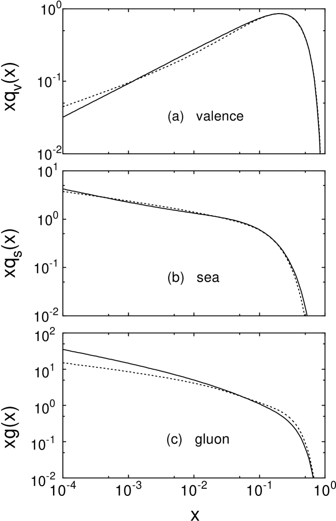
FIG. 1.: The (a) valence, (b) sea, and (c) gluon distributions in a proton are given at $Q^{2}=p_{0}^{2}=4$ GeV² for the GRV 94 LO (solid) and MRST LO (dashed) sets.

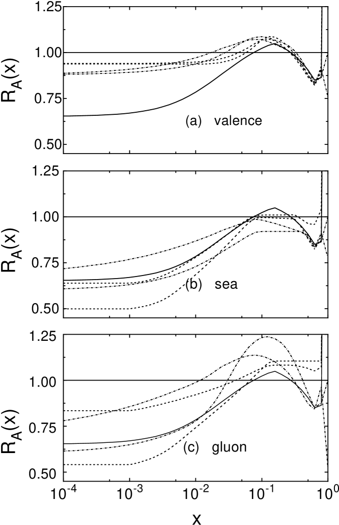
FIG. 2.: The three shadowing parameterizations for $A=200$ for (a) valence quarks, (b) sea quarks, and (c) gluons, relative to $S=1$. The $S_{1}$ parameterization is shown in the solid curves. The $S_{2}$ ratios are given by the dashed curves. At low $x$, the lower curves are for $Q=2$ GeV while the upper are for $Q=10$ GeV. The $S_{3}$ ratios, in the dot-dashed curves, are shown for the $u_{V}$ and $\overline{u}$. The lower curves at low $x$ are for $Q=1.5$ GeV while the upper curves at low $x$ are for $Q=10$ GeV.

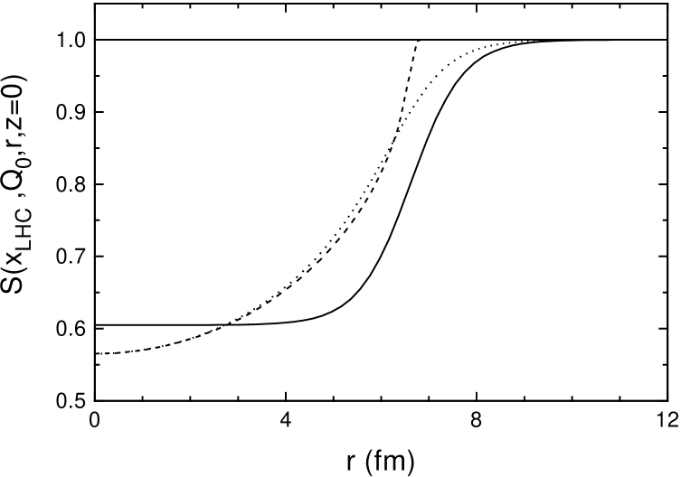
FIG. 3.: The radial distribution of shadowing for three models: $S_{\rm WS}$, Eq. (3), (solid), $S_{\rm R}$, Eq. (7) (dashed) and $S_{\rho}$, Eq. (4). All curves are normalized to a homogeneous $S^{i}(A,x,Q^{2})$ of 0.7. Note that $S_{\rm WS}$ is evaluated at $z=0$.

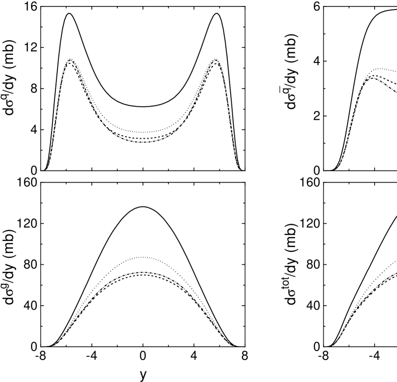
FIG. 4.: The rapidity distributions of quarks, antiquarks, gluons and the sum of all contributions in Pb+Pb collisions at $\sqrt{s_{NN}}=5.5$ TeV integrated over $b$ and divided by $AB$ calculated with the GRV 94 LO parton distributions for $p_{0}=2$ GeV. The solid curve is without shadowing, the dashed is with shadowing parameterization $S_{1}$, the dot-dashed is with $S_{2}$ and the dotted uses $S_{3}$.

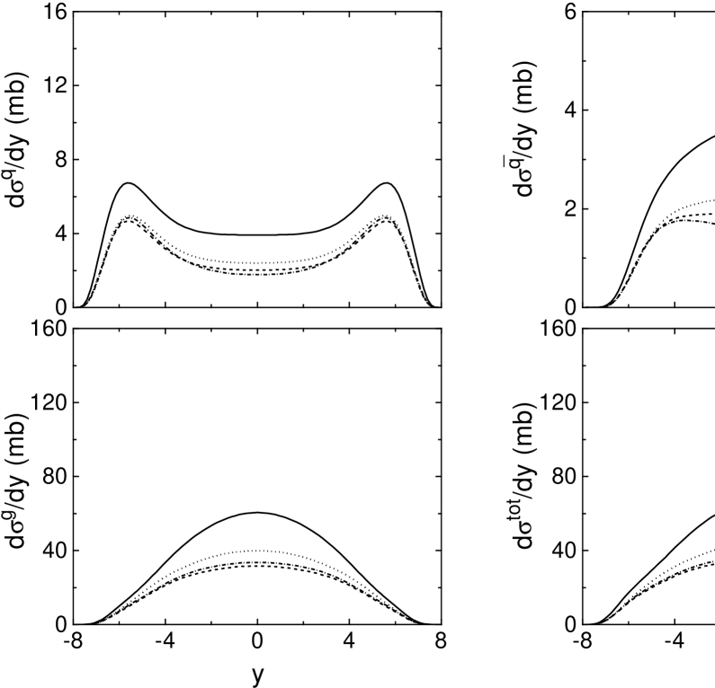
FIG. 5.: The rapidity distributions of quarks, antiquarks, gluons and the sum of all contributions in Pb+Pb collisions at $\sqrt{s_{NN}}=5.5$ TeV integrated over $b$ and divided by $AB$ calculated with the MRST LO parton distributions for $p_{0}=2$ GeV. The solid curve is without shadowing, the dashed is with shadowing parameterization $S_{1}$, the dot-dashed is with $S_{2}$ and the dotted uses $S_{3}$.

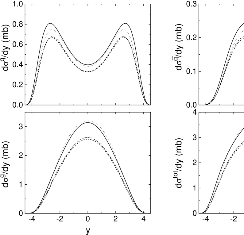
FIG. 6.: The rapidity distributions of quarks, antiquarks, gluons and the sum of all contributions in Au+Au collisions at $\sqrt{s_{NN}}=200$ GeV integrated over $b$ and divided by $AB$ calculated with the GRV 94 LO parton distributions for $p_{0}=2$ GeV. The solid curve is without shadowing, the dashed is with shadowing parameterization $S_{1}$, the dot-dashed is with $S_{2}$ and the dotted uses $S_{3}$.

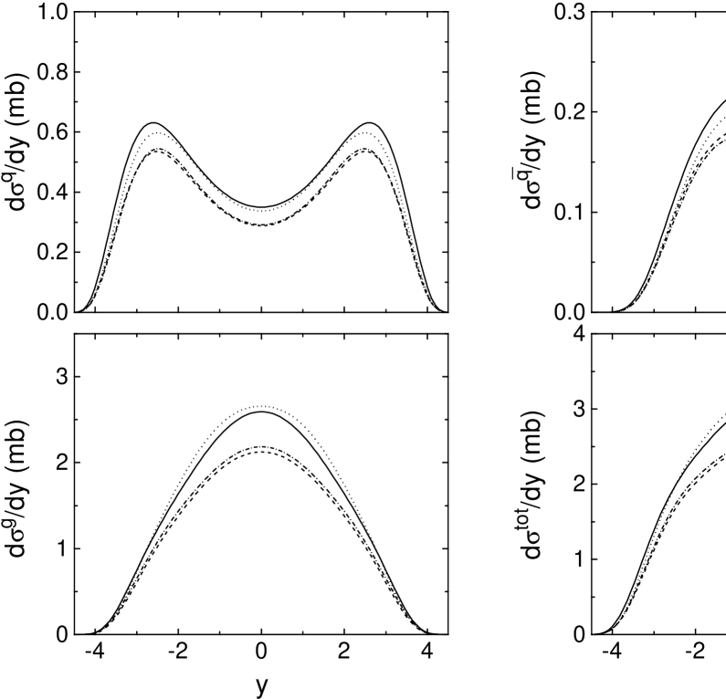
FIG. 7.: The rapidity distributions of quarks, antiquarks, gluons and the sum of all contributions in Au+Au collisions at $\sqrt{s_{NN}}=200$ GeV integrated over $b$ and divided by $AB$ calculated with the MRST LO parton distribution for $p_{0}=2$ GeV. The solid curve is without shadowing, the dashed is with shadowing parameterization $S_{1}$, the dot-dashed is with $S_{2}$ and the dotted uses $S_{3}$.

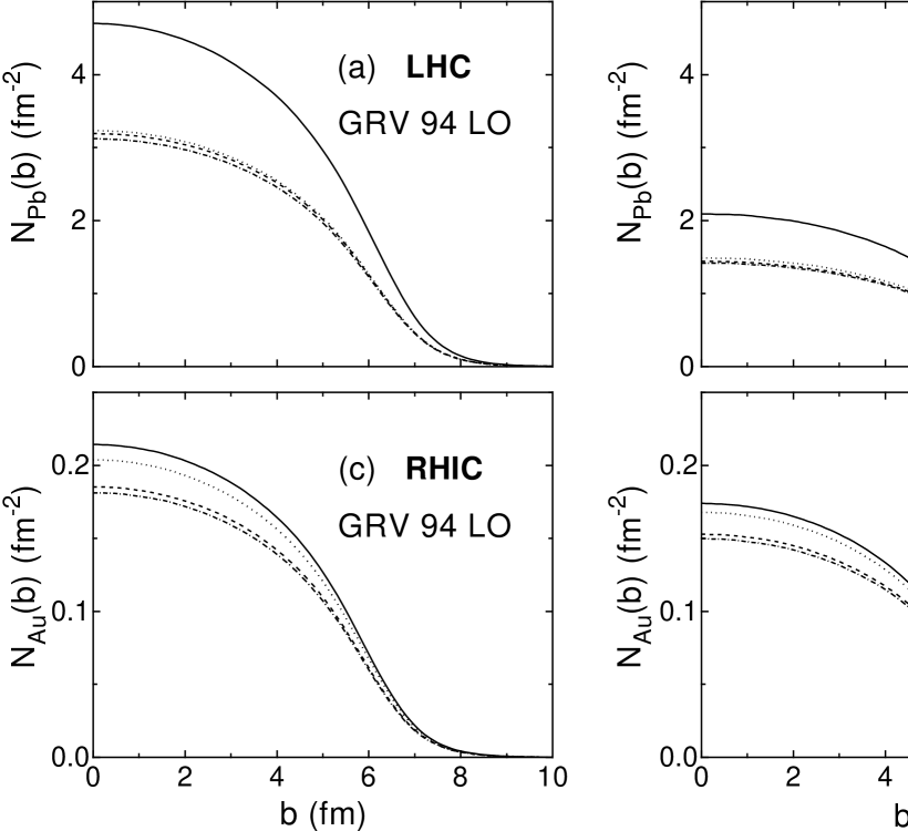
FIG. 8.: The number of scatters suffered by an incoming gluon as a function of impact parameter. The LHC results at $x_{1}=10^{-2}$ are shown in (a) and (b) for GRV 94 LO and MRST LO parton densities respectively while the RHIC calculations at $x_{1}=10^{-1}$ are shown in (c) and (d) for the GRV 94 LO and MRST LO sets. The solid curve is without shadowing, the dashed is with shadowing parameterization $S_{1}$, the dot-dashed is with $S_{2}$ and the dotted uses $S_{3}$.

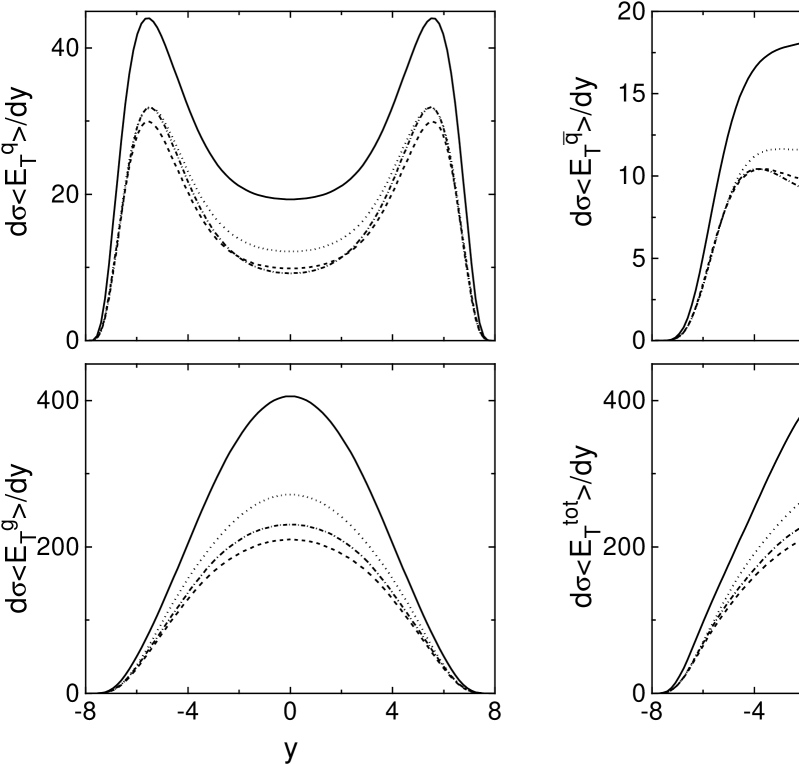
FIG. 9.: The first $E_{T}$ moment, $\sigma(p_{0})\langle E_{T}^{f}\rangle$, as a function of rapidity for quarks, antiquarks, gluons and the sum of all contributions in Pb+Pb collisions at $\sqrt{s_{NN}}=5.5$ TeV integrated over $b$ and divided by $AB$ calculated with the GRV 94 LO parton distributions for $p_{0}=2$ GeV. The solid curve is without shadowing, the dashed is with shadowing parameterization $S_{1}$, the dot-dashed is with $S_{2}$ and the dotted uses $S_{3}$.

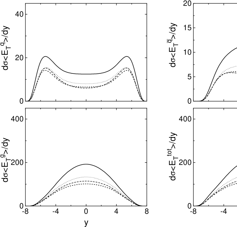
FIG. 10.: The first $E_{T}$ moment, $\sigma(p_{0})\langle E_{T}^{f}\rangle$, as a function of rapidity for quarks, antiquarks, gluons and the sum of all contributions in Pb+Pb collisions at $\sqrt{s_{NN}}=5.5$ TeV integrated over $b$ and divided by $AB$ calculated with the MRST LO parton distributions for $p_{0}=2$ GeV. The solid curve is without shadowing, the dashed is with shadowing parameterization $S_{1}$, the dot-dashed is with $S_{2}$ and the dotted uses $S_{3}$.

FIG. 11.: The first $E_{T}$ moment, $\sigma(p_{0})\langle E_{T}^{f}\rangle$, as a function of rapidity for quarks, antiquarks, gluons and the sum of all contributions in Au+Au collisions at $\sqrt{s_{NN}}=200$ GeV integrated over $b$ and divided by $AB$ calculated with the GRV 94 LO parton distributions for $p_{0}=2$ GeV. The solid curve is without shadowing, the dashed is with shadowing parameterization $S_{1}$, the dot-dashed is with $S_{2}$ and the dotted uses $S_{3}$.

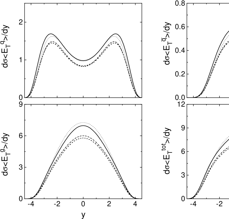
FIG. 12.: The first $E_{T}$ moment, $\sigma(p_{0})\langle E_{T}^{f}\rangle$, as a function of rapidity for quarks, antiquarks, gluons and the sum of all contributions in Au+Au collisions at $\sqrt{s_{NN}}=200$ GeV integrated over $b$ and divided by $AB$ calculated with the MRST LO parton distributions for $p_{0}=2$ GeV. The solid curve is without shadowing, the dashed is with shadowing parameterization $S_{1}$, the dot-dashed is with $S_{2}$ and the dotted uses $S_{3}$.

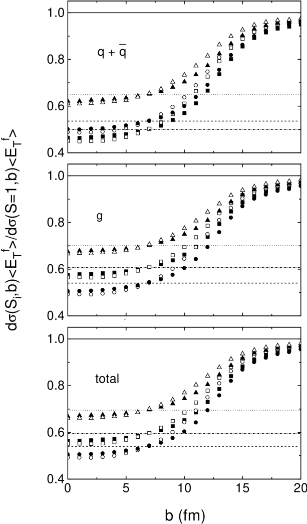
FIG. 13.: The impact parameter dependence of the first $E_{T}$ moment, $\sigma(p_{0})\langle E_{T}^{f}\rangle$ relative to the $E_{T}$ moment with $S=1$ in CMS, $|y|\leq 2.4$, calculated with the MRST LO distributions with $p_{0}=2$ GeV. The upper plot shows the ratio for quarks and antiquarks, the middle plot is the gluon ratio and the lower plot is for the total. The horizontal lines show the homogeneous shadowing results: dashed for $S_{1}$, dot-dashed for $S_{2}$, and dotted for $S_{3}$. The inhomogeneous shadowing results for $S_{1}$, circles, $S_{2}$, squares, and $S_{3}$, diamonds are shown for $S_{\rm WS}$ (filled symbols) and $S_{\rho}$ (open symbols).

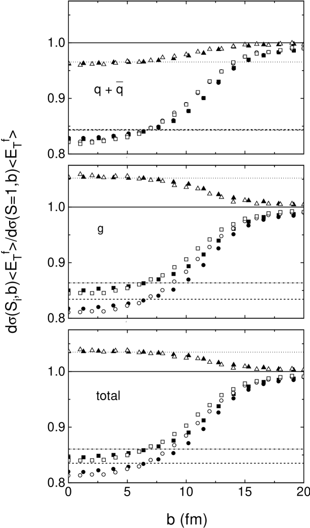
FIG. 14.: The impact parameter dependence of the first $E_{T}$ moment, $\sigma(p_{0})\langle E_{T}^{f}\rangle$ relative to the $E_{T}$ moment with $S=1$ in STAR, $|y|\leq 0.9$, calculated with the MRST LO distributions with $p_{0}=2$ GeV. The upper plot shows the ratio for quarks and antiquarks, the middle plot is the gluon ratio and the lower plot is for the total. The horizontal lines show the homogeneous shadowing results: dashed for $S_{1}$, dot-dashed for $S_{2}$, and dotted for $S_{3}$. The inhomogeneous shadowing results for $S_{1}$, circles, $S_{2}$, squares, and $S_{3}$, diamonds are shown for $S_{\rm WS}$ (filled symbols) and $S_{\rho}$ (open symbols).

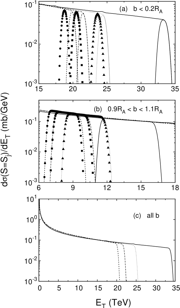
FIG. 15.: The $E_{T}$ distribution predicted for the CMS detector in the interval $|y|\leq 2.4$, calculated with the MRST LO distributions and $p_{0}=2$ GeV. The upper plot is for central collisions with $b<0.2R_{A}$, the middle plot shows the region $0.9R_{A}<b<1.1R_{A}$, and the lower plot shows the entire $E_{T}$ distribution. The lines indicate the homogeneous shadowing results: solid for no shadowing, dashed line for $S_{1}$, dot-dashed for $S_{2}$, and dotted for $S_{3}$. The inhomogeneous shadowing results for $S_{1}$, circles, $S_{2}$, squares, and $S_{3}$, diamonds are shown for $S_{\rm WS}$.

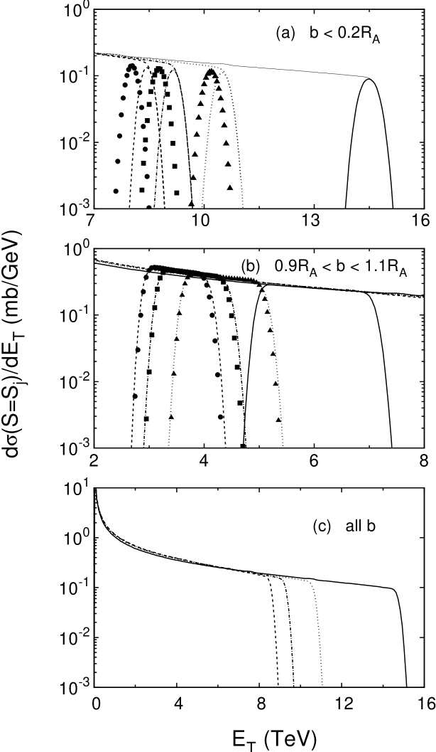
FIG. 16.: The $E_{T}$ distribution predicted for the ALICE detector in the interval $|y|\leq 1$, calculated with the MRST LO distributions and $p_{0}=2$ GeV. The upper plot shows central collisions with $b<0.2R_{A}$, the middle plot shows the region $0.9R_{A}<b<1.1R_{A}$, and the lower plot shows the entire $E_{T}$ distribution. The lines indicate the homogeneous shadowing results: solid for no shadowing, dashed line for $S_{1}$, dot-dashed for $S_{2}$, and dotted for $S_{3}$. The inhomogeneous shadowing results for $S_{1}$, circles, $S_{2}$, squares, and $S_{3}$, diamonds are shown for $S_{\rm WS}$.

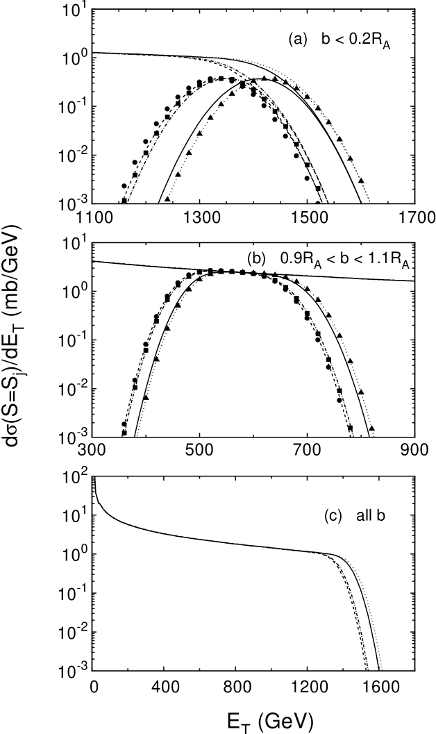
FIG. 17.: The $E_{T}$ distribution predicted for the STAR detector in the interval $|y|\leq 0.9$, calculated with the MRST LO distributions and $p_{0}=2$ GeV. The upper plot is for central collisions with $b<0.2R_{A}$, the middle plot shows the region $0.9R_{A}<b<1.1R_{A}$, and the lower plot shows the entire $E_{T}$ distribution. The lines indicate the homogeneous shadowing results: solid for no shadowing, dashed line for $S_{1}$, dot-dashed for $S_{2}$, and dotted for $S_{3}$. The inhomogeneous shadowing results for $S_{1}$, circles, $S_{2}$, squares, and $S_{3}$, diamonds are shown for $S_{\rm WS}$.

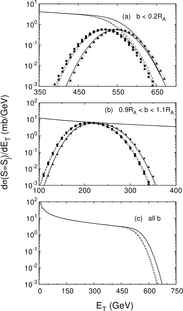
FIG. 18.: The $E_{T}$ distribution predicted for the PHENIX detector in the interval $|y|\leq 0.35$, calculated with the MRST LO distributions and $p_{0}=2$ GeV. The upper plot emphasizes central collisions with $b<0.2R_{A}$, the middle plot shows the region $0.9R_{A}<b<1.1R_{A}$, and the lower plot shows the entire $E_{T}$ distribution. The lines indicate the homogeneous shadowing results: solid for no shadowing, dashed line for $S_{1}$, dot-dashed for $S_{2}$, and dotted for $S_{3}$. The inhomogeneous shadowing results for $S_{1}$, circles, $S_{2}$, squares, and $S_{3}$, diamonds are shown for $S_{\rm WS}$.

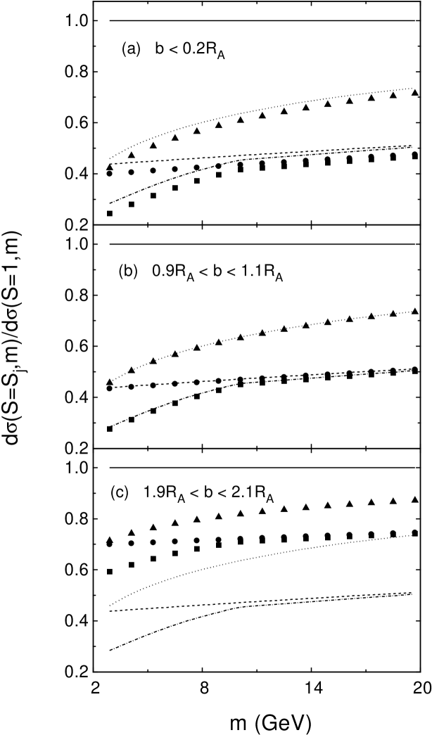
FIG. 19.: The Drell-Yan mass distribution relative to $S=1$ in ALICE, $|y|\leq 1$, calculated with the MRST LO distributions. The upper plot shows central collisions with $b<0.2R_{A}$, the middle plot shows the region $0.9R_{A}<b<1.1R_{A}$, and the lower plot shows the peripheral region $1.9R_{A}<b<2.1R_{A}$. The lines are the homogeneous shadowing result. The dashed line represents $S_{1}$, the dot-dashed, $S_{2}$, and the dotted, $S_{3}$. Equation (3) is used to calculate the inhomogeneous shadowing ratios for $S_{1,{\rm WS}}$, circles, $S_{2,{\rm WS}}$, squares, and $S_{3,{\rm WS}}$, triangles.

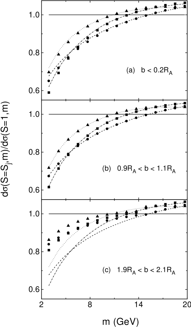
FIG. 20.: The Drell-Yan mass distribution compared to the distribution with $S=1$ in PHENIX, $|y|\leq 0.35$, calculated with the MRST LO distributions. The upper plot shows central collisions with $b<0.2R_{A}$, the middle plot shows the region $0.9R_{A}<b<1.1R_{A}$, and the lower plot shows the peripheral region $1.9R_{A}<b<2.1R_{A}$. The lines indicate the homogeneous shadowing result. The dashed line represents $S_{1}$, the dot-dashed, $S_{2}$, and the dotted, $S_{3}$. Equation (3) is used to calculate the inhomogeneous shadowing ratios for $S_{1,{\rm WS}}$, circles, $S_{2,{\rm WS}}$, squares, and $S_{3,{\rm WS}}$, diamonds.

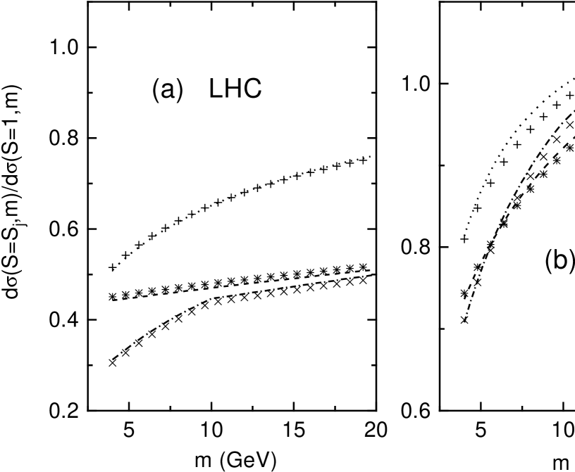
FIG. 21.: The Drell-Yan mass distribution compared to the distribution with $S=1$ at the LHC, $|y|\leq 1.$, and RHIC, $|y|\leq 0.35$ calculated with the MRST distributions. The ratios are shown at leading and next-to-leading order in the Drell-Yan cross section for homogeneous shadowing. The dashed line represents $S_{1}$, the dot-dashed, $S_{2}$, and the dotted, $S_{3}$ ratios at leading order. The next-to-leading order ratios are indicated by the symbols, $*$ ($S_{1}$), $\times$ ($S_{2}$), and $+$ ($S_{3}$).

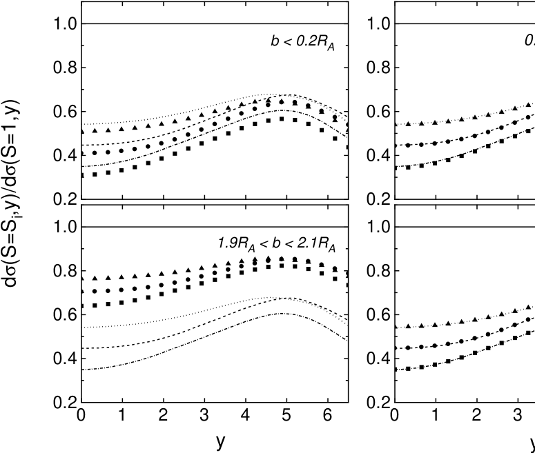
FIG. 22.: The Drell-Yan rapidity distribution in the mass interval $4<m<9$ GeV, relative to $S=1$ for Pb+Pb collisions at the LHC, calculated with the MRST LO distributions. Central, $b<0.2R_{A}$, semi-central, $0.9R_{A}<b<1.1R_{A}$, peripheral, $1.9R_{A}<b<2.1R_{A}$ impact parameters are shown along with the integral over all $b$. The lines indicate the homogeneous shadowing result. The dashed line represents $S_{1}$, the dot-dashed, $S_{2}$, and the dotted, $S_{3}$. Equation (3) is used to calculate the inhomogeneous shadowing ratios for $S_{1}$, circles, $S_{2}$, squares, and $S_{3}$, diamonds.

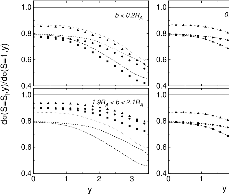
FIG. 23.: The Drell-Yan rapidity distribution in the mass interval $4<m<9$ GeV, compared to the distribution with $S=1$ in Au+Au collisions at RHIC, calculated with the MRST LO distributions. Central, $b<0.2R_{A}$, semi-central, $0.9R_{A}<b<1.1R_{A}$, peripheral, $1.9R_{A}<b<2.1R_{A}$ impact parameters are shown along with the integral over all $b$. The lines indicate the homogeneous shadowing result. The dashed line represents $S_{1}$, the dot-dashed, $S_{2}$, and the dotted, $S_{3}$. Equation (3) is used to calculate the ratio for $S_{1}$, circles, $S_{2}$, squares, and $S_{3}$, diamonds.

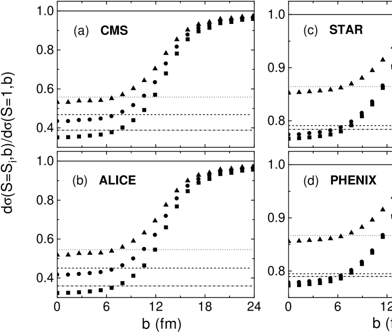
FIG. 24.: The impact parameter dependence of the Drell-Yan cross section for $4<m<9$ GeV, calculated with the MRST LO distributions. Results are shown for the central rapidity coverages of all four detectors. The lines indicate the homogeneous shadowing result: dashed for $S_{1}$, dot-dashed for $S_{2}$, and dotted for $S_{3}$. Equation (3) is used to calculate the ratio for $S_{1}$, circles, $S_{2}$, squares, and $S_{3}$, diamonds.

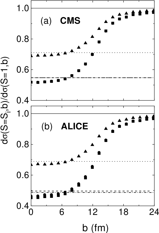
FIG. 25.: The impact parameter dependence of the Drell-Yan cross section for $11<m<20$ GeV, calculated with the MRST LO distributions. Results are shown for the central rapidity coverages of the two LHC detectors. The lines indicate the homogeneous shadowing result: dashed for $S_{1}$, dot-dashed for $S_{2}$ and dotted for $S_{3}$. Equation (3) is used to calculate the ratio for $S_{1}$, circles, $S_{2}$, squares, and $S_{3}$, diamonds.

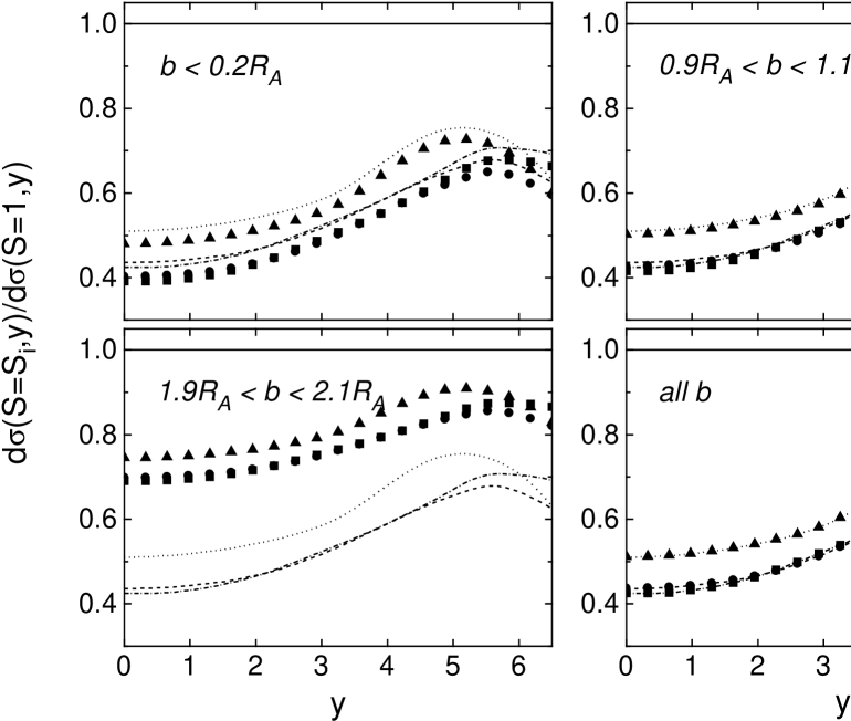
FIG. 26.: The $J/\psi$ rapidity distribution calculated in the color evaporation model with the MRST LO distributions, compared to the distribution with $S=1$ in Pb+Pb collisions at the LHC. Central, $b<0.2R_{A}$, semi-central, $0.9R_{A}<b<1.1R_{A}$, peripheral, $1.9R_{A}<b<2.1R_{A}$ impact parameters are shown along with the integral over all $b$. The lines show the homogeneous shadowing result: dashed line for $S_{1}$, dot-dashed for $S_{2}$, and dotted for $S_{3}$. Equation (3) is used to calculate the ratio for $S_{1}$, circles, $S_{2}$, squares, and $S_{3}$, diamonds.

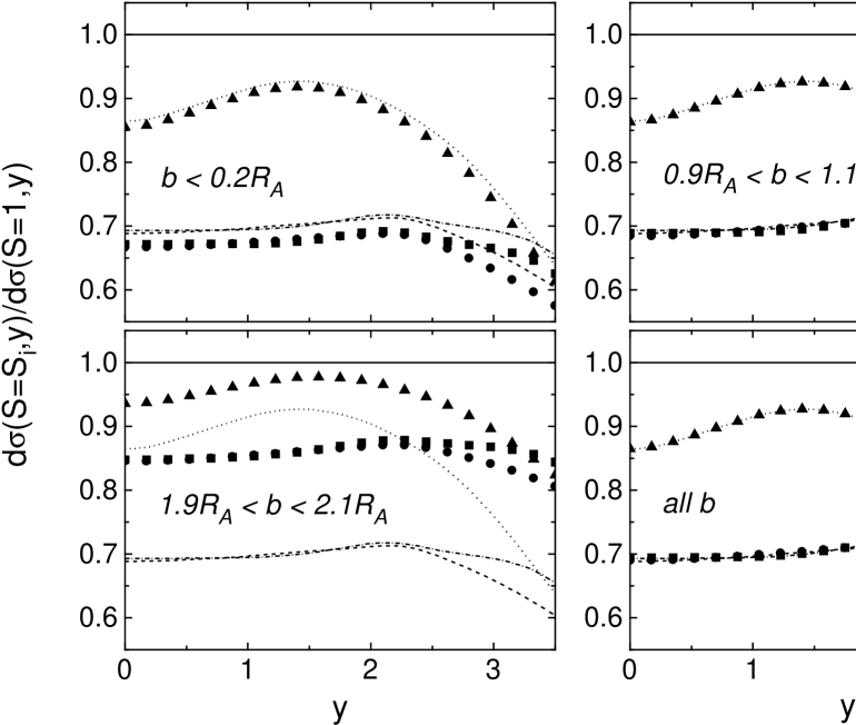
FIG. 27.: The $J/\psi$ rapidity distribution calculated in the color evaporation model with the MRST LO distributions, compared to the distribution with $S=1$ in Au+Au collisions at RHIC. Central, $b<0.2R_{A}$, semi-central, $0.9R_{A}<b<1.1R_{A}$, peripheral, $1.9R_{A}<b<2.1R_{A}$ impact parameters are shown along with the integral over all $b$. The lines show the homogeneous shadowing result: dashed line for $S_{1}$, dot-dashed for $S_{2}$, and dotted for $S_{3}$. Equation (3) is used to calculate the ratio for $S_{1}$, circles, $S_{2}$, squares, and $S_{3}$, diamonds.

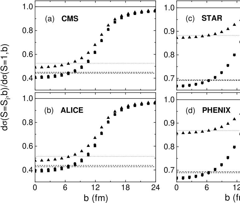
FIG. 28.: The impact parameter dependence of $J/\psi$ production calculated in the color evaporation model with the MRST LO distributions. Results are shown for the central rapidity coverages given for all four detectors. The lines show the homogeneous shadowing result: dashed line for $S_{1}$, dot-dashed for $S_{2}$, and dotted for $S_{3}$. Equation (3) is used to calculate the ratio for $S_{1}$, circles, $S_{2}$, squares, and $S_{3}$, diamonds.

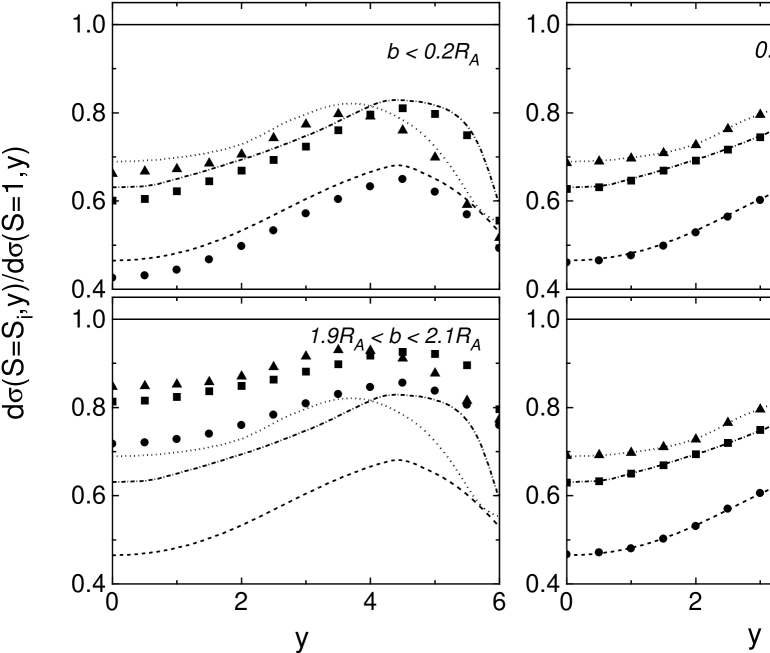
FIG. 29.: The $\Upsilon$ rapidity distribution calculated in the color evaporation model with the MRST LO distributions, compared to the distribution with $S=1$ in Pb+Pb collisions at the LHC. Central, $b<0.2R_{A}$, semi-central, $0.9R_{A}<b<1.1R_{A}$, peripheral, $1.9R_{A}<b<2.1R_{A}$ impact parameters are shown along with the integral over all $b$. The lines show the homogeneous shadowing result: dashed line for $S_{1}$, dot-dashed for $S_{2}$, and dotted for $S_{3}$. Equation (3) is used to calculate the ratio for $S_{1}$, circles, $S_{2}$, squares, and $S_{3}$, diamonds.

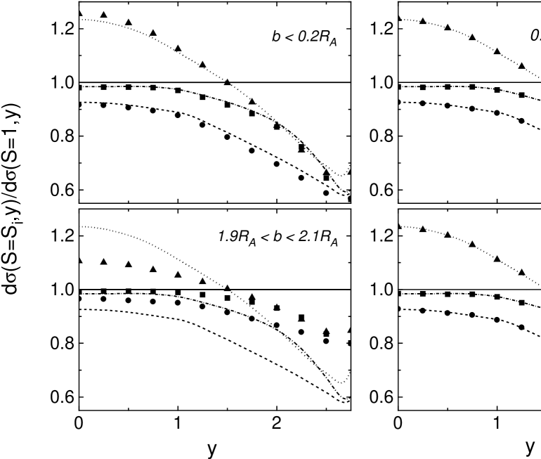
FIG. 30.: The $\Upsilon$ rapidity distribution calculated in the color evaporation model with the MRST LO distributions, compared to the distribution with $S=1$ in Au+Au collisions at RHIC. Central, $b<0.2R_{A}$, semi-central, $0.9R_{A}<b<1.1R_{A}$, peripheral, $1.9R_{A}<b<2.1R_{A}$ impact parameters are shown along with the integral over all $b$. The lines show the homogeneous shadowing result: dashed line for $S_{1}$, dot-dashed for $S_{2}$, and dotted for $S_{3}$. Equation (3) is used to calculate the ratio for $S_{1}$, circles, $S_{2}$, squares, and $S_{3}$, diamonds.

FIG. 31.: The impact parameter dependence of $\Upsilon$ production calculated in the color evaporation model with the MRST LO distributions. Results are shown for the central rapidity coverages given for all four detectors. The lines show the homogeneous shadowing result: dashed line for $S_{1}$, dot-dashed for $S_{2}$, and dotted for $S_{3}$. Equation (3) is used to calculate the ratio for $S_{1}$, circles, $S_{2}$, squares, and $S_{3}$, diamonds.

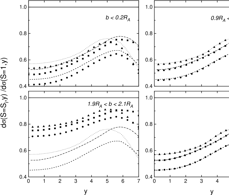
FIG. 32.: The $J/\psi$ rapidity distribution calculated in the NRQCD model with the CTEQ 3L distributions, compared to the distribution with $S=1$ in Pb+Pb collisions at the LHC. Central, $b<0.2R_{A}$, semi-central, $0.9R_{A}<b<1.1R_{A}$, peripheral, $1.9R_{A}<b<2.1R_{A}$ impact parameters are shown along with the integral over all $b$. The lines show the homogeneous shadowing result: dashed line for $S_{1}$, dot-dashed for $S_{2}$, and dotted for $S_{3}$. Equation (3) is used to calculate the ratio for $S_{1}$, circles, $S_{2}$, squares, and $S_{3}$, triangles.

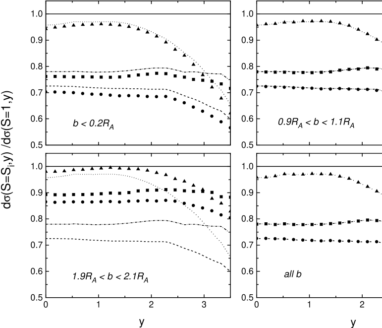
FIG. 33.: The $J/\psi$ rapidity distribution calculated in the NRQCD model with the CTEQ 3L distributions, compared to the distribution with $S=1$ in Au+Au collisions at RHIC. Central, $b<0.2R_{A}$, semi-central, $0.9R_{A}<b<1.1R_{A}$, peripheral, $1.9R_{A}<b<2.1R_{A}$ impact parameters are shown along with the integral over all $b$. The lines show the homogeneous shadowing result: dashed line for $S_{1}$, dot-dashed for $S_{2}$, and dotted for $S_{3}$. Equation (3) calculate the ratio for $S_{1}$, circles, $S_{2}$, squares, and $S_{3}$, triangles.

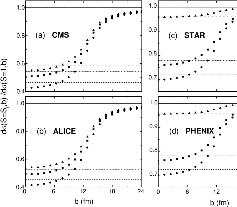
FIG. 34.: The impact parameter dependence of $J/\psi$ production calculated in NRQCD with the CTEQ 3L distributions. Results are shown for the central rapidity coverages given for all four detectors. The lines show the homogeneous shadowing result: dashed line for $S_{1}$, dot-dashed for $S_{2}$, and dotted for $S_{3}$. Equation (3) is used to calculate the ratio for $S_{1}$, circles, $S_{2}$, squares, and $S_{3}$, triangles.

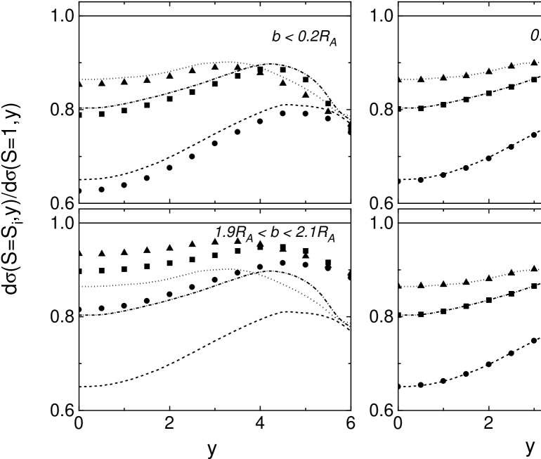
FIG. 35.: The $\Upsilon$ rapidity distribution calculated in the NRQCD model with the CTEQ 3L distributions, compared to the distribution with $S=1$ in Pb+Pb collisions at the LHC. Central, $b<0.2R_{A}$, semi-central, $0.9R_{A}<b<1.1R_{A}$, peripheral, $1.9R_{A}<b<2.1R_{A}$ impact parameters are shown along with the integral over all $b$. The lines show the homogeneous shadowing result: dashed line for $S_{1}$, dot-dashed for $S_{2}$, and dotted for $S_{3}$. Equation (3) is used to calculate the ratio for $S_{1}$, circles, $S_{2}$, squares, and $S_{3}$, triangles.

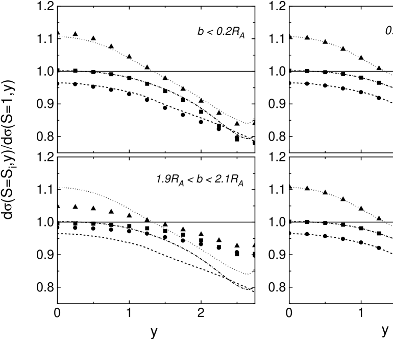
FIG. 36.: The $\Upsilon$ rapidity distribution calculated in the NRQCD model with the CTEQ 3L distributions, compared to the distribution with $S=1$ in Au+Au collisions at RHIC. Central, $b<0.2R_{A}$, semi-central, $0.9R_{A}<b<1.1R_{A}$, peripheral, $1.9R_{A}<b<2.1R_{A}$ impact parameters are shown along with the integral over all $b$. The lines show the homogeneous shadowing result: dashed line for $S_{1}$, dot-dashed for $S_{2}$, and dotted for $S_{3}$. Equation (3) calculate the ratio for $S_{1}$, circles, $S_{2}$, squares, and $S_{3}$, triangles.

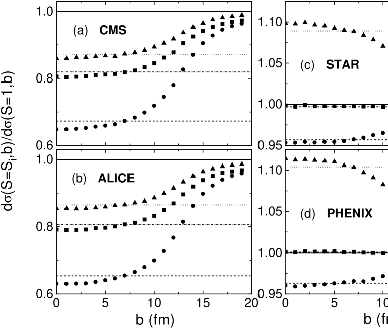
FIG. 37.: The impact parameter dependence of $\Upsilon$ production calculated in NRQCD with the CTEQ 3L distributions. Results are shown for the central rapidity coverages given for all four detectors. The lines show the homogeneous shadowing result: dashed line for $S_{1}$, dot-dashed for $S_{2}$, and dotted for $S_{3}$. Equation (3) is used to calculate the ratio for $S_{1}$, circles, $S_{2}$, squares, and $S_{3}$, triangles.

REFERENCES

- [1] J.J. Aubert et al., Nucl. Phys. B293 740, (1987); M. Arneodo, Phys. Rep. 240 301, (1994).
- [2] T. Kitagaki et al., Phys. Lett. 214, 281 (1988).
- [3] V. Emel’yanov, A. Khodinov, S.R. Klein and R. Vogt, Phys. Rev. C56, 2726 (1997).
- [4] V. Emel’yanov, A. Khodinov and M. Strikhanov, Yad. Fiz. 60, 539 (1997) [Phys. of Atomic Nuclei, 60 465, (1997)].
- [5] V. Emel’yanov, A. Khodinov, S.R. Klein and R. Vogt, Phys. Rev. Lett. 81, 1801 (1998).
- [6] C.W. deJager, H. deVries, and C. deVries, Atomic Data and Nuclear Data Tables 14 485, (1974).
- [7] C. Adloff et al. (H1 Collab.), Nucl. Phys. B497 3, (1997); J. Breitweg et al. (ZEUS Collab.), Eur. Phys. J. C7 609, (1999).
- [8] M. Glück, E. Reya, and A. Vogt, Z. Phys. C67 433, (1995).
- [9] A.D. Martin, R.G. Roberts, and W.J. Stirling, and R.S. Thorne, Eur. Phys. J. C4 (1998) 463; Phys. Lett. B443 (1998) 301.
- [10] K.J. Eskola, J. Qiu, and J. Czyzewski, private communication.
- [11] D.W. Duke and J.F. Owens, Phys. Rev. D30 49, (1984).
- [12] K.J. Eskola, Nucl. Phys. B400 240, (1993).
- [13] M. Glück, E. Reya, and A. Vogt, Z. Phys. C53 127, (1992).
- [14] K.J. Eskola, V.J. Kolhinen and P.V. Ruuskanen, Nucl. Phys. B535 351, (1998).
- [15] K.J. Eskola, V.J. Kolhinen and C.A. Salgado, Eur. Phys. J. C9 (1999) 61.
- [16] L.V. Gribov, E.M. Levin, and M.G. Ryskin, Phys. Rep. 100 1, (1983).
- [17] A. L. Ayala, M. B. Gay Ducati and E. M. Levin, Nucl. Phys. B493, 305 (1997).
- [18] Z. Huang, H. Jung Lu and I. Sarcevic, Nucl. Phys. A637 79, (1998).
- [19] L.D. Landau and I.Ya. Pomeranchuk, Dokl. Akad. Nauk SSSR 92 535, 735, (1953); A.B. Migdal, Phys. Rev. 103 1811, (1956); S.R. Klein, hep-ph/9802442, Rev. Mod. Phys. in press.
- [20] D. Kahana, in proceedings of RHIC Summer Study ’96: Theory Workshop on Relativistic Heavy Ion Collisions, edited by D.E. Kahana and Y. Pang, BNL-52514, p. 175; Y. Pang, ibid, p. 193.
- [21] S. Kumano and F.E. Close, Phys. Rev. C 41 1855, (1990).
- [22] G.L. Li, K.F. Liu and G.E. Brown, Phys. Lett. B213, 531 (1988).
- [23] K.J. Eskola and M. Gyulassy, Phys. Rev. C47 2329, (1993).
- [24] K.J. Eskola and K. Kajantie, Z. Phys. C75 515, (1997); K.J. Eskola, K. Kajantie and J. Lindfors, Nucl. Phys. B323 37, (1989).
- [25] K.J. Eskola and X.-N. Wang, Int. J. Mod. Phys. A10 2881, (1995).
- [26] A. Leonidov and D. Ostrovsky, hep-ph/9811417.
- [27] K.J. Eskola, B. Müller, and X.-N. Wang, Phys. Lett. B374 20, (1996).
- [28] K.J. Eskola, R. Vogt, and X.-N. Wang, Int. J. Mod. Phys. A10 3087, (1995); R. Vogt, nucl-th/9903051, Heavy Ion Phys., in press.
- [29] J. Breitweg et al. (ZEUS Collab.), Eur. Phys. J. C7 609, (1999).
- [30] M. Banner et al. (UA2 Collab.), Phys. Lett. B118 203, (1982).
- [31] A. Leonidov, in proceedings of the RIKEN/BNL workshop on ‘Hard Parton Physics in High Energy Nuclear Collisions’, BNL, 1999.
- [32] CMS Technical Proposal, CERN/LHCC 94-38 (1994).
- [33] ALICE Technical Proposal, CERN/LHCC/95-71 (1995); ALICE Addendum to the Technical Proposal, CERN/LHCC/96-32 (1996); A. Morsch et al. (ALICE Collab.), Nucl. Phys. A638 571c, (1998).
- [34] STAR Conceptual Design Report, LBL PUB-5347, 1992; H. Wieman et al. (STAR Collab.), Nucl. Phys. A638 559c, (1998).
- [35] PHENIX Conceptual Design Report, 1993 (unpublished).
- [36] N. Hammon, H. Stöcker and W. Greiner, hep-ph/9903527.
- [37] J.D. Bjorken, Phys. Rev. D27 140, (1983).
- [38] K.J. Eskola, K. Kajantie and P.V. Ruuskanen, Phys. Lett. B332 191, (1994).
- [39] M. Gyulassy and X.-N. Wang, Phys. Rev. D44, 3501 (1991).
- [40] H.R. Schmidt et al., Z. Phys. C38, 109 (1988).
- [41] R. Albrecht et al., Z. Phys. C38 3, (1988); J. Schukraft, Z. Phys. C38 59, (1988); A. Bamberger et al., Z. Phys. C38 89, (1988).
- [42] C. Caso et al., Eur. Phys. J. C3 1, (1998).
- [43] T. Akesson et al., Phys. Lett. B214, 295 (1988).
- [44] G. Baym, G. Friedman and I. Sarcevic, Phys. Lett. B219, 205 (1989).
- [45] A. Capella, A. Kaidalov and J. Tran Thanh Van, hep-ph/9903244, submitted to Heavy Ion Physics.
- [46] T.S. Biro, E. van Doorn, B. Müller, M.H. Thoma and X.-N. Wang, Phys. Rev. C48, 1275 (1993).
- [47] V. Emel’yanov, A. Khodinov, S. Klein and R. Vogt, Phys. Rev. C59, R1860 (1999).
- [48] S. Gavin et al., Int. J. Mod. Phys. A10 2961 (1995).
- [49] R.V. Gavai, D. Kharzeev, H. Satz, G. Schuler, K. Sridhar and R. Vogt, Int. J. Mod. Phys. A10 3043, (1995); G.A. Schuler and R. Vogt, Phys. Lett. B387 181, (1996).
- [50] B.L. Combridge, Nucl. Phys. B151 429, (1979).
- [51] R. Vogt, LBNL-42294, hep-ph/9907317.
- [52] R. Baier and R. Rückl, Z. Phys. C19 251, (1983); G.A. Schuler, CERN Preprint, CERN-TH.7170/94.
- [53] G.T. Bodwin, E. Braaten and G.P. Lepage, Phys. Rev. D51 1125, (1995).
- [54] H.L. Lai, J. Botts, J. Huston, J. G. Morfin, J. F. Owens, J. W. Qiu, W. K. Tung and H. Weerts, Phys. Rev. D51 4763, (1995).
- [55] M. Beneke and I.Z. Rothstein, Phys. Rev. D54 2005, (1996).