Dynamical Renormalization Group Approach to Quantum Kinetics in Scalar and Gauge Theories

Abstract

We derive quantum kinetic equations from a quantum field theory implementing a diagrammatic perturbative expansion improved by a resummation via the dynamical renormalization group. The method begins by obtaining the equation of motion of the distribution function in perturbation theory. The solution of this equation of motion reveals secular terms that grow in time, the dynamical renormalization group resums these secular terms in real time and leads directly to the quantum kinetic equation. This method allows to include consistently medium effects via resummations akin to hard thermal loops but away from equilibrium. A close relationship between this approach and the renormalization group in Euclidean field theory is established. In particular, coarse graining, stationary solutions, relaxation time approximation and relaxation rates have a natural parallel as irrelevant operators, fixed points, linearization and stability exponents in the Euclidean renormalization group, respectively. We used this method to study the relaxation in a cool gas of pions and sigma mesons in the $O(4)$ chiral linear sigma model. We obtain in relaxation time approximation the pion and sigma meson relaxation rates. We also find that in large momentum limit emission and absorption of massless pions result in threshold infrared divergence in sigma meson relaxation rate and lead to a crossover behavior in relaxation. We then study the relaxation of charged quasiparticles in scalar electrodynamics (SQED). We begin with a gauge invariant description of the distribution function and implement the hard thermal loop resummation for longitudinal and transverse photons as well as for the scalars. While longitudinal, Debye screened photons lead to purely exponential relaxation, transverse photons, only dynamically screened by Landau damping lead to anomalous (non-exponential) relaxation, thus leading to a crossover between two different relaxational regimes. We emphasize that infrared divergent damping rates are indicative of non-exponential relaxation and the dynamical renormalization group reveals the correct relaxation directly in real time. Furthermore the relaxational time scales for charged quasiparticles are similar to those found in QCD in a self-consistent HTL resummation. Finally we also show that this method provides a natural framework to interpret and resolve the issue of pinch singularities out of equilibrium and establish a direct correspondence between pinch singularities and secular terms in time-dependent perturbation theory. We argue that this method is particularly well suited to study quantum kinetics and transport in gauge theories.

I Introduction

The search for the quark-gluon plasma (QGP) at the Relativistic Heavy Ion Collider (RHIC) and the forthcoming Large Hadron Collider (LHC) has the potential of providing clear evidence for the formation of a deconfined plasma of quarks and gluons and hopefully to study the chiral phase transition. Perhaps this is the only opportunity to study phase transitions that are conjectured to occur in particle physics with earth-bound accelerators and an intense theoretical effort has developed parallel to the experimental program that seeks to understand the signatures of the QGP and the chiral phase transition [1, 2]. An important part of the program is to assess whether the plasma, once formed, achieves a state of thermodynamic equilibrium and if so on what time scales. This is an important question since current estimates suggest that at the energies and luminosities to be achieved at RHIC, the spatial and temporal scales for the existence of the QGP are of the order of $20~{}\mbox{fm}$ [1]. The description of the space-time evolution in an ultrarelativistic heavy ion collision requires the understanding of phenomena on different time and spatial scales. Ideally, such a description should begin from the parton distribution functions of the colliding nuclei as the initial state and evolve this state in time using QCD to obtain the kinetic and chemical equilibration of partons, the emergence of hydrodynamics and the hadronization and freeze-out stages [3]. An important part of the program to study the space-time evolution from first principles seeks to establish a consistent kinetic description of transport phenomena in a dense partonic environment. Such kinetic description has the potential of providing a detailed understanding of collective flow, observables (hadronic and electromagnetic) such as multiparticle distributions, charmonium suppression, freeze out of hadrons and other important experimental signatures that will lead to an unambiguous determination of whether a QGP has been formed and the observables of phase transitions. This premise justifies an important theoretical effort to obtain such a kinetic description from first principles. During the last few years there have been important advances in this program, from derivations of kinetic and transport equations from first principles in QCD [3, 4, 5, 6] and scalar field theories [7, 8, 9, 10] to numerical codes that describe the space-time evolution in terms of partonic cascades [3] that include screening corrections in the scattering cross sections [11, 12] and more recently nonequilibrium dynamics has been studied via lattice simulations [13, 14, 15, 16]

The kinetic description to study hot and/or dense quantum field theory systems is also of fundamental importance in the understanding of the emergence of hydrodynamics in the long-wavelength limit of a quantum field theory [17] and more recently a transport approach has been advocated as a description of the collective dynamics of soft degrees of freedom in hot QCD [19, 18, 20, 22, 21]. The typical approach to derive transport equations begins by introducing a Wigner transform of a particular nonequilibrium Green’s functions at two different space-time points [3, 4, 5, 20, 23] (a gauge covariant Wigner transform in the case of gauge theories) and often requires a quasiparticle approximation [5, 23]. The rationale behind a Wigner transform of a nonequilibrium Green’s function is the assumption of a wide separation between the microscopic (fast) and relaxational (slow) time scales, typically justified in a weakly coupled theory. A recent derivation of transport equations for a hot QCD plasma along these lines has recently been reported in [20], however the collisional terms obtained in the quasiparticle and relaxation time approximations turn out to be infrared divergent.

Thus, the importance of a fundamental understanding of transport in quantum field theory from first principles, with the direct application to the experimental aspects of the search for the QGP justifies the study of transport phenomena from many different perspectives. In this article we present a novel method to obtain quantum kinetic equations directly from the underlying quantum field theory implementing a dynamical renormalization group resummation. Such approach has been recently introduced to study the relaxation of mean-fields of hard charged scalars in a gauge theory [24]. This method allowed to obtain directly in Ref. [24] the anomalous relaxation of hard charged excitations in an Abelian gauge theory [25], providing an interpretation of infrared divergent damping rates [26] in terms of non-exponential relaxation and pointed to a shortcoming in the interpretation of quasiparticle relaxation in terms of complex poles in the propagator. Infrared divergences associated with the emission and absorption of long-wavelength gauge bosons are ubiquitous in gauge theories. Thus, this novel approach is particularly suitable to study transport phenomena in gauge theories.

Goals and Strategy: The goals of this article are to provide a novel and alternative derivation of quantum kinetic equations directly from the microscopic quantum field theory in real time and apply this program to several relevant cases of interest. We consider scalar theories describing pions and sigma mesons and gauge theories. This approach allows to include consistently medium effects, such as nonequilibrium generalizations of the hard thermal loop resummation, describes anomalous relaxation and reveals the proper time scales for relaxation directly in real time. There are several advantages that this program offers as compared to other approaches to transport phenomena:

• (i) It allows to study the crossover between different relaxational behavior in real time. This is relevant in the case of resonances where the medium may enhance threshold effects.

• (ii) It describes non-exponential relaxation in a clear manner and treats threshold effects consistently, providing a real-time interpretation of infrared divergent damping rates in gauge theories,

• (iii) It provides a systematic field-theoretical method to include higher order corrections and allows to incorporate self-consistently medium effects such as for example a resummation of hard thermal loops [27, 28, 29] that are necessary to determine the relevant degrees of freedom and their microscopic time scales.

• (iv) It resolves the issue of pinch singularities that often appear in calculations of physical quantities out of equilibrium.

The strategy to be followed is a generalization of the methods introduced in Ref. [24] but adapted to the description of quantum kinetics. The starting point is the identification of the distribution function of the quasiparticles which could require a resummation of medium effects (the equivalent of hard thermal loops [27, 28, 29]). The equation of motion for this distribution function is solved in a perturbative expansion in terms of nonequilibrium Feynman diagrams. The perturbative solution in real time displays secular terms, i.e., terms that grow in time and invalidate the perturbative expansion beyond a particular time scale (recognized a posteriori to be the relaxational time scale). The dynamical renormalization group implements a systematic resummation of these secular terms and the resulting renormalization group equation is the quantum kinetic equation.

The validity of this approach hinges upon the basic assumption of a wide separation between the microscopic and the relaxational time scales. Such an assumption underlies every approach to a kinetic description and is generally justified in weakly coupled theories. Unlike other approaches in terms of a truncation of the equations of motion for the Wigner distribution function, the main ingredient in the approach presented here is a perturbative diagrammatic evaluation of the time evolution of the proper distribution function in real time [8] improved via a renormalization group resummation of the secular divergences.

An important bonus of this approach is that it illuminates the origin and provides a natural resolution of pinch singularities [30, 31] found in perturbation theory out of equilibrium. The perturbative real-time approach combined with the renormalization group resummation reveal clearly that these are indicative of the nonequilibrium evolution of the distribution functions. In this framework, pinch singularities are the manifestation of secular terms.

The article is organized as follows: In Sec. II we summarize the main ingredients of nonequilibrium field theory to establish the perturbative framework. In Sec. III we study the familiar case of a scalar field theory, including in addition the nonequilibrium resummation akin to the hard thermal loops to account for the effective masses in the medium and therefore the relevant microscopic time scales. In Sec. IV we discuss in detail the main features of the dynamical renormalization group approach to quantum kinetics, compare it to the more familiar renormalization group of Euclidean quantum field theory and provide an easy-to-follow recipe to obtain quantum kinetic equations. In Sec. V we apply these techniques to obtain the kinetic equations for cool pions and sigma mesons in the $O(4)$ linear sigma model in the chiral limit. In relaxation time approximation we obtain the relaxation rates for pions and sigma mesons. This case allows us to highlight the power of this approach to study threshold effects on the relaxation of resonances, in particular the crossover between two different relaxational regimes as a function of the momentum of the resonance. This aspect becomes phenomenological important in view of the recent studies by Hatsuda and collaborators [32] that reveal a dropping of the sigma mass near the chiral phase transition and an enhancement of threshold effects with potential observational consequences in heavy ion collisions.

In Sec. VI we study the relaxation of charged quasiparticles in the full range of momenta in SQED. This theory has the same hard thermal loop structure at lowest order as QED and QCD [33, 34, 35, 36] and shares many features of these theories such as the lack of magnetic screening mass. In particular, in this Abelian case we provide a gauge invariant description of the quasiparticle distribution function, thus bypassing the complications associated with the gauge covariant Wigner transforms of the charged field Green’s function. The hard thermal loop resummation [27, 28, 29] is included in the scalar as well as in the gauge boson spectral densities. We find that the exchange of HTL resummed longitudinal photons leads to exponential relaxation but the exchange of dynamically screened transverse photons leads to anomalous relaxation, thus leading to a crossover behavior in the relaxation of the distribution function as a function of the momentum of the charged particle. The real-time description of relaxation advocated in this article bypasses the ambiguities associated with an infrared divergent damping rate [20, 34]. In Sec. VII we discuss the issue of pinch singularities found in calculations in nonequilibrium field theory and establish the equivalence between these and secular terms in the perturbative expansion, these singularities are thus resolved via the resummation provided by the dynamical renormalization group.

We summarize our results and discuss further implications and future directions in the conclusions.

II Real-time Nonequilibrium Techniques

The field theoretical methods to describe nonequilibrium processes have been studied at length in the literature to which the reader should refer for a more detailed presentation [30, 37, 38, 39, 40, 41, 42, 43]. Here we only highlight those aspects and details that are necessary for our purposes.

The basic ingredient is the time evolution of density matrix prepared initially at time $t=t_{0}$, which leads to the generating functional of nonequilibrium Green’s functions in terms of a path integral defined on a contour in the complex time plane.

The contour has two branches running forward and backward in the real time axis corresponding to the unitary evolution operator forward in time that pre-multiplies the density matrix at $t_{0}$ and the hermitian conjugate that post-multiplies it and determines evolution backwards in time. The initial density matrix determines the boundary conditions on the propagators.

This is a standard formulation of nonequilibrium quantum field theory known as Schwinger-Keldysh or closed-time-path (CTP) [30, 37, 38, 39, 40, 41, 42, 43]. Fields defined on the forward and backward branches are labeled respectively with “$+$” and “$-$” superscripts and are treated independently. Introducing sources on the CTP contour, one can easily construct the nonequilibrium generating functional, which generates nonequilibrium Green’s functions through functional derivatives with respect to sources much in the same manner as the usual formulation of amplitudes in terms of path integrals.

The path integral along the CTP contour is in terms of the effective Lagrangian defined by

$${\cal{L}}_{\text{noneq}}[{\Psi}^{+},{\Psi}^{-}]={\cal{L}}[{\Psi}^{+}]-{\cal L}[{\Psi}^{-}]~{},$$ (1)

where ${\cal L}[\Psi]$ denotes the corresponding Lagrangian in usual field theory and $\Psi$ denotes any generic (bosonic or fermionic) field. The advantage of the path integral representation with the above nonequilibrium, effective Lagrangian is that it is straightforward to construct diagrammatically a perturbative expansion of the nonequilibrium Green’s functions in terms of modified nonequilibrium Feynman rules. These nonequilibrium Feynman rules are as follows.

• (i) The number of vertices is doubled: Those associated with fields on the “$+$” branch are the usual interaction vertices, while those associated with fields on the “$-$” branch have the opposite sign.

• (ii) There are four propagators corresponding to the possible contractions of fields among the two branches. Besides the usual time-ordered (Feynman) propagators which are associated with fields on the “$+$” branch, there are anti-time ordered propagators associated with fields on the “$-$” branch and the Wightman functions associated with fields on different branches.

• (iii) The combinatoric factors of the Feynman diagrams are the same as those in the usual calculation of S-matrix elements in field theory.

For a scalar (bosonic) field $\Phi(x)$, the spatial Fourier transform of the nonequilibrium propagators are defined by (the extension to the case of a gauge or fermionic field is straightforward)

$$G_{\bf k}^{>}(t,t^{\prime})=i\int d^{3}x\,e^{-i{\bf k}\cdot{\bf x}}\,\Big{\langle}\Phi({{\bf x}},t)\Phi({{\bf 0}},t^{\prime})\Big{\rangle}~{},$$ (3)

$$G_{\bf k}^{<}(t,t^{\prime})=i\int d^{3}x\,e^{-i{\bf k}\cdot{\bf x}}\,\Big{\langle}\Phi({{\bf 0}},t^{\prime})\Phi({{\bf x}},t)\Big{\rangle}~{},$$ (4)

$$G_{\bf k}^{++}(t,t^{\prime})=G_{\bf k}^{>}(t,t^{\prime})\theta(t-t^{\prime})+G_{\bf k}^{<}(t,t^{\prime})\theta(t^{\prime}-t)\,,$$ (5)

$$G_{\bf k}^{--}(t,t^{\prime})=G_{\bf k}^{>}(t,t^{\prime})\theta(t^{\prime}-t)+G_{\bf k}^{<}(t,t^{\prime})\theta(t-t^{\prime})~{},$$ (6)

$$G_{\bf k}^{+-}(t,t^{\prime})=G_{\bf k}^{<}(t,t^{\prime})~{},$$ (7)

$$G_{\bf k}^{-+}(t,t^{\prime})=G_{\bf k}^{>}(t,t^{\prime})~{},$$ (8)

where $\langle\cdots\rangle$ denotes the expectation value with respect to the initial density matrix. From the definitions of the nonequilibrium propagators eqs. (II), it is clear that they satisfy the identity:

$$G_{\bf k}^{++}(t,t^{\prime})+G_{\bf k}^{--}(t,t^{\prime})-G_{\bf k}^{+-}(t,t^{\prime})-G_{\bf k}^{-+}(t,t^{\prime})=0~{}.$$ (9)

The retarded and advanced propagators are defined as

$$G_{{\rm R},\bf k}(t,t^{\prime}) = G_{\bf k}^{++}(t,t^{\prime})-G_{\bf k}^{+-}(t,t^{\prime})=\left[G_{\bf k}^{>}(t,t^{\prime})-G_{\bf k}^{<}(t,t^{\prime})\right]\theta(t-t^{\prime})~{},$$

$$G_{{\rm A},\bf k}(t,t^{\prime}) = G_{\bf k}^{++}(t,t^{\prime})-G_{\bf k}^{-+}(t,t^{\prime})=\left[G_{\bf k}^{<}(t,t^{\prime})-G_{\bf k}^{>}(t,t^{\prime})\right]\theta(t^{\prime}-t)~{},$$

which are useful in the discussion of the pinch singularities discussed in a later section (see Sec. VII).

It now remains to specify the initial state. If we were considering the situation in equilibrium the natural initial density matrix would describe a thermal initial state for the free particles at temperature $T$. The density matrix of this initial state is $\hat{\rho}=\exp(-H_{0}/T)$, where $H_{0}$ is the free Hamiltonian of the system, and the time evolution is with the full interacting Hamiltonian. This is tantamount to switching on the interaction at $t=t_{0}$. If the full Hamiltonian does not commute with $H_{0}$ the density matrix evolves out of equilibrium for $t>t_{0}$. This choice of the thermal initial state for the free particles determines the usual Kubo-Martin-Schwinger (KMS) conditions on the Green’s functions:

$$G_{\bf k}^{<}(t,t^{\prime})=G_{\bf k}^{>}(t-i\beta,t^{\prime})~{}.$$ (10)

Perturbative expansions are carried out with the following real-time equilibrium free quasiparticle Green’s functions:

$$G_{\bf k}^{>}(t,t^{\prime}) = \frac{i}{2\omega_{\bf k}}\left\{[1+n_{B}(\omega_{\bf k})]\;e^{-i\omega_{\bf k}(t-t^{\prime})}+n_{B}(\omega_{\bf k})\;e^{i\omega_{\bf k}(t-t^{\prime})}\right\}~{}~{},$$ (12)

$$G_{\bf k}^{<}(t,t^{\prime}) = \frac{i}{2\omega_{\bf k}}\left\{n_{B}(\omega_{\bf k})~{}e^{-i\omega_{\bf k}(t-t^{\prime})}+[1+n_{B}(\omega_{\bf k})]\;e^{i\omega_{\bf k}(t-t^{\prime})}\right\}~{}~{},$$ (13)

$$\omega_{\bf k} = \sqrt{k^{2}+m^{2}}~{},\quad\quad\quad n_{B}(\omega)=[\exp(\beta\omega)-1]^{-1}~{},$$ (14)

where (here and henceforth) $k=|{\bf k}|$, and $m$ is the mass of the field and $n_{B}(\omega)$ is the equilibrium Bose-Einstein distribution function.

In a hot and/or dense medium the definition of the quasiparticles whose distribution function we want to study may require a resummation scheme such as for example that of hard thermal loops generalized to nonequilibrium situations. In these cases, the Hamiltonian is rearranged in such a way that part of the interaction is self-consistently included in the part of the Hamiltonian that commutes with the quasiparticle number operator, call it for convenience $H_{0}$ and specific counterterms are included in the interacting part $H_{I}$ to avoid double counting.

As we are interested in obtaining an equation of evolution for a quasiparticle distribution function, the most natural initial state corresponds to a density matrix that is diagonal in the basis of free quasiparticles, i.e. that commutes with $H_{0}$. This initial density matrix is then evolved in time with the full Hamiltonian, and if the interaction does not commute with $H_{0}$ the distribution function of these quasiparticles will evolve in time.

The distribution function $n_{\bf k}(t_{0})$ is the expectation value of the operator that counts these quasiparticles in the initial density matrix. Under the assumption that the initial density matrix is diagonal in the basis of this quasiparticle number, perturbative expansions are carried out with the following nonequilibrium free quasiparticle Green’s functions:

$$G_{\bf k}^{>}(t,t^{\prime}) = \frac{i}{2\omega_{\bf k}}\left\{[1+n_{\bf k}(t_{0})]\;e^{-i\omega_{\bf k}(t-t^{\prime})}+n_{\bf k}(t_{0})\;e^{i\omega_{\bf k}(t-t^{\prime})}\right\}~{},$$ (16)

$$G_{\bf k}^{<}(t,t^{\prime}) = \frac{i}{2\omega_{\bf k}}\left\{n_{\bf k}(t_{0})\;e^{-i\omega_{\bf k}(t-t^{\prime})}+[1+n_{\bf k}(t_{0})]\;e^{i\omega_{\bf k}(t-t^{\prime})}\right\}~{}~{},$$ (17)

where $\omega_{\bf k}$ is the dispersion relation for the free quasiparticle. In this picture the width of the quasiparticles arises from their interaction and is related to the relaxation rate of the distribution function in relaxation time approximation. This point will become more clear in the sections that follow where we implement this program in detail.

Finally, it is easy to check that the (bosonic) free quasiparticle Green’s functions, eqs. (II) and (II), satisfy

$$G_{\bf k}^{>}(t,t^{\prime})=G_{\bf k}^{<}(t^{\prime},t)~{},$$ (18)

which will be useful in our following calculations.

III Self-interacting Scalar Theory

We begin our investigation with a self-interacting scalar theory. The Lagrangian density is given by

$${\cal{L}}[\Phi]=\frac{1}{2}\left(\partial_{\mu}\Phi\right)^{2}-\frac{1}{2}m^{2}_{0}\Phi^{2}-\frac{\lambda}{4!}\Phi^{4}~{},$$ (19)

where $m_{0}$ is the bare mass.

As mentioned in the introduction, the first step towards understanding the kinetic regime is the identification of the microscopic time scales in the problem. In a medium, the bare particles are dressed by the interactions becoming quasiparticles. One is interested in describing the relaxation of these quasiparticles. Thus the important microscopic time scales are those associated with the quasiparticles and not the bare particles. If a kinetic equation is obtained in some perturbative scheme, such a scheme should be in terms of the quasiparticles which already implies a resummation of the perturbative expansion. This is precisely the rationale behind the resummation of the hard thermal loops in finite temperature field theory [27, 28, 29] and also behind the self-consistent treatment [7, 8].

In a scalar field theory in equilibrium such a self-consistent resummation can be implemented by writing in the Lagrangian

$$m^{2}_{0}=m^{2}_{\rm eff}+\delta m^{2}~{},$$ (20)

where $m_{\rm eff}$ is the renormalized and temperature dependent quasiparticle thermal effective mass which enters in the propagators, and $\delta m^{2}$ is a counterterm which will cancel a subset of Feynman diagrams in the perturbative expansion and is considered part of the interaction Lagrangian. As shown in Ref. [44] for the scalar field theory case, this method implements a resummation akin to the hard thermal loops in a gauge theory [27, 28, 29]. Parwani showed [44] that this resummation is effectively implemented by solving the following self-consistent gap equation for $m^{2}_{\rm eff}$ [8, 44, 45]

$$m^{2}_{\rm eff}=m^{2}_{0}+\frac{\lambda}{2}\langle\Phi^{2}\rangle~{},\quad\langle\Phi^{2}\rangle=\int\frac{d^{3}q}{(2\pi)^{3}}\frac{1+2\,n_{B}(\omega_{\bf k})}{2\omega_{\bf k}}~{},$$ (21)

with $\omega_{\bf k}=\sqrt{k^{2}+m^{2}_{\rm eff}}$. The divergences (quadratic and logarithmic in terms of a spatial momentum cutoff) in the zero-temperature part of eq. (21) can be absorbed into a renormalization of the bare mass by a subtraction at some renormalization scale. A convenient choice corresponds to a renormalization scale at $T=0$ and $m(T=0)=m$ is the zero-temperature mass.

For $T\gg m_{\rm eff}$, the solution of the gap equation is given by [44, 45]

$$m^{2}_{\rm eff}=m^{2}+{\lambda\over 2}\left[\ \frac{T^{2}}{12}-\frac{m_{\rm eff}\,T}{4\pi}+{\cal{O}}\left(m^{2}_{\rm eff}\ln\left[\frac{m_{\rm eff}}{T}\right]\right)\right]~{}.$$ (22)

In particular, for $T\gg\sqrt{\lambda}\;T\gg m$, we can neglect the zero-temperature mass $m$ and obtain

$$m^{2}_{\rm eff}=\frac{\lambda\;T^{2}}{24}+{\cal{O}}\left(\lambda^{3/2}T^{2}\right)~{}.$$ (23)

In the massless case, $m_{\rm eff}$ serves as an infrared cutoff for the loop integrals [44, 46]. The leading term of eq. (23) provides the correct microscopic time scale at large temperature.

We note that this renormalized and temperature dependent mass determines the important time scales in the medium but is not the position of the quasiparticle pole (or, strictly speaking, resonance).

When the temperature is much larger than the renormalized zero temperature mass, the hard thermal loop resummation is needed to incorporate the physically relevant time and length scales in the perturbative expansion. For a hard quasiparticle $k\sim T$, while for a soft quasiparticle $k\lesssim\sqrt{\lambda}\;T$, hence the longest microscopic time scale of the system is $t_{\rm micro}\sim 1/\sqrt{\lambda}\;T\sim 1/m_{\rm eff}$.

A Quantum kinetic equation

In this subsection we obtain the evolution equations for the distribution functions of quasiparticles. For this we consider an initial state out of equilibrium described by a density matrix that is diagonal in the basis of the free quasiparticles, but with nonequilibrium distribution functions. If the medium is hot these quasiparticles will have an effective mass $m_{\rm eff}$ which will result from medium effects, much in the same manner as the temperature dependent thermal mass in the equilibrium situation described above. This mass will be very different from the bare mass $m_{0}$ in the absence of medium effects and must be taken into account for the correct assessment of the microscopic time scales. Thus, we write the Hamiltonian in terms of the in medium dressed mass $m_{\rm eff}$ and a counterterm $\delta m^{2}=m^{2}_{0}-m^{2}_{\rm eff}$ which will be treated as part of the perturbation and required to cancel the mass shifts consistently in perturbation theory. This is the nonequilibrium generalization of the resummation described above in the equilibrium case. We emphasize that $m^{2}_{\rm eff}$ depends on the initial distribution of quasiparticles. This observation will become important later when we discuss the time evolution of the distribution functions and therefore of the effective mass.

We write the Hamiltonian of the theory as

$$H=H_{0}+H_{\text{int}}~{},$$ (25)

$$H_{0}=\frac{1}{2}\int d^{3}x\left[\Pi^{2}+({\bf\nabla}\Phi)^{2}+m^{2}_{\rm eff}\;\Phi^{2}\right]~{},$$ (26)

$$H_{\text{int}}=\int d^{3}x\left[\frac{\lambda}{4!}\;\Phi^{4}+\frac{1}{2}\delta m^{2}\;\Phi^{2}\right]~{},$$ (27)

where $\Pi({\bf x},t)=\dot{\Phi}({\bf x},t)$ is the canonical momentum, and the mass counterterm has been absorbed in the interaction. Here and henceforth, a dot denotes derivative with respect to time. The free part of the Hamiltonian $H_{0}$ describes free quasiparticles of renormalized finite-temperature mass $m_{\rm eff}$ and is diagonal and Gaussian in terms of free quasiparticle creation and annihilation of operators $a^{\dagger}({\bf k})$ and $a({\bf k})$.

With this definition, the lifetime of the quasiparticles will be a consequence of interactions. In this manner, the nonequilibrium equivalent of the hard thermal loops (in the sense that the distribution functions are non-thermal) which in this theory amount to local terms, have been absorbed in the definition of the effective mass. This guarantees that the microscopic time scales are explicit in the quasiparticle Hamiltonian.

As discussed in the previous section, we consider that the initial density matrix at time $t=t_{0}$, is diagonal in the basis of free quasiparticles, but with out of equilibrium initial distribution functions $n_{\bf k}(t_{0})$. The Heisenberg field operators at time $t$ are now written as

$$\Phi({\bf x},t) = \int\frac{d^{3}k}{(2\pi)^{3/2}}\;\Phi({\bf k},t)\;e^{i{\bf k}\cdot{\bf x}}~{},\quad\quad\Phi({\bf k},t)=\frac{1}{\sqrt{2\omega_{\bf k}}}\left[a({\bf k},t)+a^{\dagger}({-\bf k},t)\right]~{},$$ (29)

$$\Pi({\bf x},t) = \int\frac{d^{3}k}{(2\pi)^{3/2}}\;\Pi({\bf k},t)\;e^{i{\bf k}\cdot{\bf x}}~{},\quad\quad\Pi({\bf k},t)=i\sqrt{\frac{\omega_{\bf k}}{2}}\left[a^{\dagger}({-\bf k},t)-a({\bf k},t)\right]~{},$$ (30)

where $a^{\dagger}({\bf k},t)$ and $a({\bf k},t)$ are, respectively, creation and annihilation operators at time $t$ and $\omega_{\bf k}=\sqrt{k^{2}+m^{2}_{\rm eff}}$. The expectation value of quasiparticle number operators $n_{\bf k}(t)$ can be expressed in terms of the field $\Phi({\bf k},t)$ and the conjugate momentum $\Pi({\bf k},t)$ as follows

$$n_{\bf k}(t) = \left\langle a^{\dagger}({\bf k},t)\,a({\bf k},t)\right\rangle$$ (31)

$$= {1\over 2\omega_{\bf k}}\biggl{\{}\left\langle\Pi({\bf k},t)\,\Pi({-\bf k},t)\right\rangle+\omega^{2}_{\bf k}\,\left\langle\Phi({\bf k},t)\,\Phi({-\bf k},t)\right\rangle$$ (33)

$$+\,i\omega_{\bf k}\Bigl{[}\left\langle\Phi({\bf k},t)\,\Pi({-\bf k},t)\right\rangle-\left\langle\Pi({\bf k},t)\,\Phi({-\bf k},t)\right\rangle\Bigr{]}\biggr{\}}~{},$$

where the bracket $\langle\cdots\rangle$ means an average over the Gaussian density matrix defined by the initial distribution functions $n_{\bf k}(t_{0})$. The time-dependent distribution (33) is interpreted as the quasiparticle distribution function.

The interaction Hamiltonian in momentum space is given by

$$H_{\text{int}}=\frac{\lambda}{4!}\frac{1}{(2\pi)^{3}}\int\prod_{i=1}^{4}d^{3}q_{i}\,\Phi({{\bf q}_{i}},t)\;\delta^{3}({\bf q}_{1}+{\bf q}_{2}+{\bf q}_{3}+{\bf q}_{4})+\frac{\delta m^{2}}{2}\int d^{3}q\,\Phi({\bf q},t)\;\Phi({-\bf q},t)~{}.$$ (34)

Taking the derivative of $n_{\bf k}(t)$ with respect to time and using the Heisenberg field equations, we find

$${\dot{n}}_{\bf k}(t) = -\frac{1}{2\omega_{\bf k}}\Bigg{[}\frac{\lambda}{6}\,\Big{\langle}[\Phi^{3}({\bf k},t)]\,\Pi({-\bf k},t)+\Pi({\bf k},t)\,[\Phi^{3}({\bf k},t)]\Big{\rangle}$$ (36)

$$+\,\delta m^{2}\,\Big{\langle}\Phi({\bf k},t)\,\Pi(-{\bf k},t)+\Pi({\bf k},t)\,\Phi({-\bf k},t)\Big{\rangle}\Bigg{]}~{},$$

where we use the compact notation:

$$[\Phi^{3}({\bf k},t)]\equiv\frac{1}{(2\pi)^{3}}\int d^{3}q_{1}\;d^{3}q_{2}\;d^{3}q_{3}\,\Phi({\bf q}_{1},t)\;\Phi({\bf q}_{2},t)\;\Phi({\bf q}_{3},t)\;\delta^{3}\left({\bf k}-{\bf q}_{1}-{\bf q}_{2}-{\bf q}_{3}\right)~{}.$$ (37)

In a perturbative expansion care is needed to handle the canonical momentum [$\Pi({\bf k},t)=\dot{\Phi}({\bf k},t)$] and the scalar field at the same time because of Schwinger terms. This ambiguity is avoided by noticing that

$$\left\langle\Pi({\bf k},t)\,[\Phi^{3}({-\bf k},t)]\right\rangle = \text{Tr}\left[\hat{\rho}(t_{0})\,\Pi_{\bf k}(t)\,[\Phi^{3}({-\bf k},t)]\right]$$ (38)

$$\equiv \lim_{t\rightarrow t^{\prime}}{\partial\over\partial t^{\prime}}\text{Tr}\left[[\Phi^{3}({-\bf k},t)]^{+}\,\hat{\rho}(t_{0})\,\Phi^{-}({\bf k},t^{\prime})\right]$$ (39)

$$= \left.{\partial\over\partial t^{\prime}}\left\langle[\Phi^{3}({-\bf k},t)]^{+}\,\Phi^{-}({\bf k},t^{\prime})\right\rangle\right|_{t^{\prime}=t}~{},$$ (40)

where we used the cyclic property of the trace and the “$\pm$” superscripts for the fields refer to field insertions obtained as variational derivatives with respect to sources in the forward ($+$) time branch and backward ($-$) time branch in the nonequilibrium generating functional.

We now use the canonical commutation relation between $\Pi$ and $\Phi$ and define the mass counterterm $\delta m^{2}=\lambda\Delta/6$ to write the above expression as

$${\dot{n}}_{\bf k}(t) = -\frac{\lambda}{12\omega_{\bf k}}\Bigg{\{}\frac{\partial}{\partial t^{\prime}}\bigg{[}2\Big{\langle}[\Phi^{3}({\bf k},t)]^{+}\,\Phi^{-}({-\bf k},t^{\prime})\Big{\rangle}+\Delta\Bigl{[}\Bigl{\langle}\Phi^{+}({\bf k},t)\Phi^{-}({-\bf k},t^{\prime})\Big{\rangle}+\Big{\langle}\Phi^{+}({\bf k},t^{\prime})\Phi^{-}({-\bf k},t)\Bigr{\rangle}\Bigr{]}\bigg{]}_{t=t^{\prime}}$$ (42)

$$+3i\int\frac{d^{3}q}{(2\pi)^{3}}\Big{\langle}\Phi^{+}({\bf q},t)\Phi^{-}({-\bf q},t)\Big{\rangle}\Bigg{\}}~{}.$$

The right-hand side of eq. (42) can be obtained perturbatively in weak coupling expansion in $\lambda$. Such a perturbative expansion is in terms of the nonequilibrium vertices and Green’s functions eqs. (II) with the basic Green’s functions given by eqs. (II). At order ${\cal O}(\lambda)$ the right hand side of (42) vanishes identically. This is a consequence of the fact that the initial density matrix is diagonal in the basis of free quasiparticles.

Figs. 1a-1c display the contributions up to two loops to the kinetic equation (42). The tadpole diagrams, depicted in Figs. 1a and 1b as well as the last term in eq. (42) are canceled by the proper choice of $\Delta$.

An important point to notice is that these Green’s functions include the proper microscopic scales as the contribution of the hard thermal loops have been incorporated by summing the tadpole diagrams. The propagators entering in the calculations are the resummed propagators. The terms with $\Delta$ are required to cancel the tadpoles to all orders.

Thus, from the formidable expression (42) only the first term remains after $\Delta$ is properly chosen in order to cancel the tadpole diagrams. This requirement guarantees that the mass in the propagators is the effective mass that includes the microscopic time scales. Hence, we find that the final form of the kinetic equation is given by

$${\dot{n}}_{\bf k}(t)=-\frac{\lambda}{6\omega_{\bf k}}\frac{\partial}{\partial t^{\prime}}\left[\Big{\langle}[\Phi^{3}({\bf k},t)]^{+}\,\Phi^{-}({-\bf k},t^{\prime})\Big{\rangle}\right]_{t=t^{\prime}}~{},$$ (43)

with the understanding that no tadpole diagrams contribute to the above equations as they are automatically canceled by the terms containing $\Delta$ in eq. (42).

To lowest order the condition that the tadpoles are canceled leads to the following condition on $\Delta$

$$\Delta=-3\int\frac{d^{3}q}{(2\pi)^{3}}\frac{1+2n_{\bf q}(t_{0})}{2\,\omega_{\bf q}}~{},$$ (44)

therefore the effective mass is the solution to the self-consistent gap equation

$$m^{2}_{\rm eff}=m^{2}_{0}+\frac{\lambda}{2}\int\frac{d^{3}q}{(2\pi)^{3}}\frac{1+2\,n_{\bf q}(t_{0})}{2\omega_{\bf q}}~{},\quad\omega_{\bf q}=\sqrt{q^{2}+m^{2}_{\rm eff}}~{}.$$ (45)

We see that the requirement that the term proportional to $\Delta$ in the kinetic equation cancels the tadpole contributions is equivalent to the hard thermal loop resummation in the equilibrium case [44] and makes explicit that $m^{2}_{\rm eff}$ is a functional of the initial nonequilibrium distribution functions.

As will be discussed in detail below, such an expansion will be meaningful for times $t\ll t_{\text{rel}}=|n_{\bf k}(t)/{\dot{n}}_{\bf k}(t)|$, where $t_{\text{rel}}$ is the relaxational time scale for the nonequilibrium distribution function. For small enough coupling we expect that $t_{\text{rel}}$ will be large enough such that there is a wide separation between the microscopic and the relaxational time scales that will warrant such an approximation (see discussion below).

To two-loop order, the time evolution of the distribution function that follows from eq.(43) is given by

$${\dot{n}}_{\bf k}(t) = \frac{\lambda^{2}}{3}\frac{1}{2\omega_{\bf k}}\,\int\frac{d^{3}q_{1}}{(2\pi)^{3}2\omega_{{\bf q}_{1}}}\frac{d^{3}q_{2}}{(2\pi)^{3}2\omega_{{\bf q}_{2}}}\frac{d^{3}q_{3}}{(2\pi)^{3}2\omega_{{\bf q}_{3}}}\int^{t}_{t_{0}}dt^{\prime\prime}~{}(2\pi)^{3}\delta^{3}({\bf k}-{\bf q}_{1}-{\bf q}_{2}-{\bf q}_{3})$$ (48)

$$\times\bigg{[}{\cal N}_{1}(t_{0})\cos[(\omega_{\bf k}+\omega_{{\bf q}_{1}}+\omega_{{\bf q}_{2}}+\omega_{{\bf q}_{3}})(t-t^{\prime\prime})]+3{\cal N}_{2}(t_{0})\cos[(\omega_{\bf k}+\omega_{{\bf q}_{1}}+\omega_{{\bf q}_{2}}-\omega_{{\bf q}_{3}})(t-t^{\prime\prime})]$$

$$+\,3{\cal N}_{3}(t_{0})\cos[(\omega_{\bf k}-\omega_{{\bf q}_{1}}-\omega_{{\bf q}_{2}}+\omega_{{\bf q}_{3}})(t-t^{\prime\prime})]+{\cal N}_{4}(t_{0})\cos[(\omega_{\bf k}-\omega_{{\bf q}_{1}}-\omega_{{\bf q}_{2}}-\omega_{{\bf q}_{3}}(t-t^{\prime\prime})]\bigg{]},$$

where

$${\cal N}_{1}(t) = [1+n_{\bf k}(t)][1+n_{{\bf q}_{1}}(t)][1+n_{{\bf q}_{2}}(t)][1+n_{{\bf q}_{3}}(t)]-n_{\bf k}(t)\;n_{{\bf q}_{1}}(t)\;n_{{\bf q}_{2}}(t)\;n_{{\bf q}_{3}}(t)~{},$$ (50)

$${\cal N}_{2}(t) = [1+n_{\bf k}(t)][1+n_{{\bf q}_{1}}(t)][1+n_{{\bf q}_{2}}(t)]\;n_{{\bf q}_{3}}(t)-n_{\bf k}(t)\;n_{{\bf q}_{1}}(t)\;n_{{\bf q}_{2}}(t)\;[1+n_{{\bf q}_{3}}(t)]~{},$$ (51)

$${\cal N}_{3}(t) = [1+n_{\bf k}(t)]\;n_{{\bf q}_{1}}(t)\;n_{{\bf q}_{2}}(t)\;[1+n_{{\bf q}_{3}}(t)]-n_{\bf k}(t)\;[1+n_{{\bf q}_{1}}(t)][1+n_{{\bf q}_{2}}(t)]\;n_{{\bf q}_{3}}(t)~{},$$ (52)

$${\cal N}_{4}(t) = [1+n_{\bf k}(t)]\;n_{{\bf q}_{1}}(t)\;n_{{\bf q}_{2}}(t)\;n_{{\bf q}_{3}}(t)-n_{\bf k}(t)\;[1+n_{{\bf q}_{1}}(t)][1+n_{{\bf q}_{2}}(t)][1+n_{{\bf q}_{3}}(t)]~{}\;.$$ (53)

The kinetic equation (48) is retarded and causal. The different contributions have a physical interpretation in terms of the ‘gain minus loss’ processes in the plasma. The first term describes the creation of four particles minus the destruction of four particles in the plasma, the second and fourth terms describe the creation of three particles and destruction of one minus destruction of three and creation of one, the third term is the scattering of two particles off two particles and is the usual Boltzmann term.

Since the propagators entering in the perturbative expansion of the kinetic equation are in terms of the distribution functions at the initial time $t_{0}$, the time integration can be done straightforwardly leading to the following equation:

$${\dot{n}}_{\bf k}(t)=\frac{\lambda^{2}}{3}\int d\omega\,{\cal R}[\omega,{\bf k};{\cal N}_{i}(t_{0})]\,\frac{\sin[(\omega-\omega_{\bf k})(t-t_{0})]}{\pi(\omega-\omega_{\bf k})}~{},$$ (54)

where ${\cal R}[\omega,{\bf k};{\cal N}_{i}(t_{0})]$ is given by

$${\cal R}[\omega,{\bf k};{\cal N}_{i}(t_{0})] = \frac{\pi}{2\omega_{\bf k}}\,\int\frac{d^{3}q_{1}}{(2\pi)^{3}2\omega_{{\bf q}_{1}}}\frac{d^{3}q_{2}}{(2\pi)^{3}2\omega_{{\bf q}_{2}}}\frac{d^{3}q_{3}}{(2\pi)^{3}2\omega_{{\bf q}_{3}}}(2\pi)^{3}\delta^{3}({\bf k}-{\bf q}_{1}-{\bf q}_{2}-{\bf q}_{3})$$ (57)

$$\times\bigg{[}\delta(\omega+\omega_{{\bf q}_{1}}+\omega_{{\bf q}_{2}}+\omega_{{\bf q}_{3}})\,{\cal N}_{1}(t_{0})+3\,\delta(\omega+\omega_{{\bf q}_{1}}+\omega_{{\bf q}_{2}}-\omega_{{\bf q}_{3}})\,{\cal N}_{2}(t_{0})$$

$$+\,3\delta(\omega-\omega_{{\bf q}_{1}}-\omega_{{\bf q}_{2}}+\omega_{{\bf q}_{3}})\,{\cal N}_{3}(t_{0})+\delta(\omega-\omega_{{\bf q}_{1}}-\omega_{{\bf q}_{2}}-\omega_{{\bf q}_{3}})\,{\cal N}_{4}(t_{0})\bigg{]}~{}.$$

We are now ready to solve the kinetic equation derived above. Since ${\cal R}[\omega,{\bf k};{\cal N}_{i}(t_{0})]$ is fixed at initial time $t_{0}$, eq.(54) can be solved by direct integration over $t$, thus leading to

$$n_{\bf k}(t)=n_{\bf k}(t_{0})+\frac{\lambda^{2}}{3}\int d\omega\,{\cal R}[\omega,{\bf k};{\cal N}_{i}(t_{0})]\frac{1-\cos[(\omega-\omega_{\bf k})(t-t_{0})]}{\pi(\omega-\omega_{\bf k})^{2}}~{}.$$ (58)

This expression gives the time evolution of the quasiparticle distribution function to lowest order in perturbation theory, but only for early times. To make this statement more precise consider the limit $t\gg t_{0}$ in the expression between brackets in (58) which can be recognized from Fermi’s Golden Rule of elementary time-dependent perturbation theory

$$\lim_{t-t_{0}\to\infty}\frac{1-\cos[(\omega-\omega_{\bf k})(t-t_{0})]}{\pi(\omega-\omega_{\bf k})^{2}}=(t-t_{0})\;\delta(\omega-\omega_{\bf k})~{}.$$ (59)

A more detailed evaluation of the long time limit is obtained by using the following expression [24]

$$\int_{-a}^{\infty}{dy\over y^{2}}\left(1-\cos yt\right)\;p(y)\buildrel t\to\infty\over{=}\pi\;t\;p(0)+{\cal P}\int_{-a}^{\infty}{dy\over y^{2}}\;[p(y)-p(0)]+{\cal O}\left({1\over t}\right)~{},$$ (60)

where $a$ is a fixed positive number, $p(y)$ is a smooth function for $-a\leq y<\infty$ and is regular at $y=0$. Thus, provided that ${\cal R}[\omega,{\bf k};{\cal N}_{i}(t_{0})]$ is finite at $\omega=\omega_{\bf k}$, we find $n_{\bf k}(t)$ is given by

$$n_{\bf k}(t) = n_{\bf k}(t_{0})+\frac{\lambda^{2}}{3}\,{\cal R}[\omega_{\bf k},{\bf k};{\cal N}_{i}(t_{0})]\,(t-t_{0})+\,\text{non-secular terms}~{}.$$ (61)

The term that grows linearly with time is a secular term, and by non-secular terms in (61) we refer to terms that are bound at all times. The approximation above, replacing the oscillatory terms with resonant denominators by $t\,\delta(\omega-\omega_{\bf k})$ is the same as that invoked in ordinary time-dependent perturbation theory leading to Fermi’s Golden Rule.

Clearly, the presence of secular terms in time restricts the validity of the perturbative expansion to a time interval $t-t_{0}\ll t_{\rm rel}$ with

$$t_{\rm rel}({\bf k})\approx\frac{3n_{\bf k}(t_{0})}{\lambda^{2}\;{\cal R}[\omega_{\bf k},{\bf k};{\cal N}_{i}(t_{0})]}~{}.$$ (62)

Since the time scales in the integral in eq.(58) are of the order of or shorter than $t_{\rm micro}\sim 1/m_{\rm eff}$ the asymptotic form given by (61) is valid for $t-t_{0}\gg t_{\rm micro}$. Therefore for weak coupling there is a regime of intermediate asymptotics in time

$$t_{\rm micro}\ll t-t_{0}\ll t_{\rm rel}({\bf k})$$ (63)

such that (i) the corrections to the distribution function is dominated by the secular term, and (ii) perturbation theory is valid.

We note two important features of this analysis:

• (i) In the intermediate asymptotic regime (63) the only explicit dependence on the initial time $t_{0}$ is in the secular term, since ${\cal R}[\omega_{\bf k},{\bf k};{\cal N}_{i}(t_{0})]$ depends on $t_{0}$ only implicitly through the initial distribution functions. These observations will become important for the analysis that follows below.

• (ii) ${\cal R}[\omega_{\bf k},{\bf k};{\cal N}_{i}(t_{0})]$ given by eq. (57) with (50)-(53) evaluated at $t_{0}$ vanishes if the initial distribution functions are the equilibrium ones as a result of the on-shell delta functions and the equilibrium relation $1+n_{B}(\omega_{\bf q})=\exp(\beta\omega_{\bf q})n_{B}(\omega_{\bf q})$, in this case there are no secular terms in the perturbative expansion.

To highlight the significance of the second point above in a manner that will allow us to establish contact with the issue of pinch singularities in a later section, we note that the secular term in eq. (61) corresponds to the net change of quasiparticles distribution function in the time interval $t-t_{0}$. To see this more explicitly, let us rewrite

$$\frac{\lambda^{2}}{3}{\cal R}[\omega_{\bf k},{\bf k};{\cal N}_{i}(t_{0})]=\frac{-i}{2\omega_{\bf k}}\Big{[}[1+n_{\bf k}(t_{0})]\,\Sigma^{<}(\omega_{\bf k},{\bf k};t_{0})-n_{\bf k}(t_{0})\,\Sigma^{>}(\omega_{\bf k},{\bf k};t_{0})\Big{]}~{},$$ (64)

where $\Sigma^{>}(\omega_{\bf k},{\bf k};t_{0})-\Sigma^{<}(\omega_{\bf k},{\bf k};t_{0})\equiv 2\,i\,{\rm Im}\Sigma_{R}(\omega_{\bf k},{\bf k};t_{0})$ with $\Sigma_{R}(\omega_{\bf k},{\bf k};t_{0})$ being the the on-shell retarded scalar self-energy [8] calculated to two-loop order in terms of the initial distribution functions $n_{\bf k}(t_{0})$. Indeed, the first and the second terms in (64), respectively, correspond to the ‘gain’ and the ‘loss’ parts in the usual Boltzmann collision term. Hence one can easily recognize that $\lambda^{2}{\cal R}[\omega_{\bf k},{\bf k};{\cal N}_{i}(t_{0})]/3$ is the net production rate of quasiparticles per unit time. Moreover, the absence of secular term for a system in thermal equilibrium [for which $n_{\bf k}(t_{0})=n_{B}(\omega_{\bf k})$] is a consequence of the KMS condition for the self-energy in thermal equilibrium:

$$\Sigma^{>}(\omega_{\bf k},{\bf k})=e^{\beta\omega_{\bf k}}\Sigma^{<}(\omega_{\bf k},{\bf k})~{}.$$ (65)

B Dynamical renormalization group: resummation of secular terms

The dynamical renormalization group is a systematic generalization of multiple scale analysis and sums the secular terms, thus improving the perturbative expansion [47, 48]. It was originally introduced to improve the asymptotic behavior of solutions of differential equations [47, 48] to study pattern formation in condensed matter systems and has since been adapted to studying the nonequilibrium evolution of mean-fields in quantum field theory [49] and the time evolution of quantum systems [50].

For discussions of the dynamical renormalization group in other contexts, including applications to problems in quantum mechanics and quantum field theory, see Refs. [47, 48, 49, 50].

In this section we implement the dynamical renormalization group resummation of secular divergences to improve the perturbative expansion following the formulation presented in Ref. [24].

This is achieved by introducing the renormalized initial distribution functions $n_{\bf p}(\tau)$, which are related to the bare initial distribution function $n_{\bf p}(t_{0})$ via a renormalization constant ${\cal Z}_{\bf p}(\tau,t_{0})$ by

$$n_{\bf p}(t_{0})={\cal Z}_{\bf p}(\tau,t_{0})\;n_{\bf p}(\tau)~{},\quad{\cal Z}_{\bf p}(\tau,t_{0})=1+\frac{\lambda^{2}}{3}\;z^{(1)}_{\bf p}(\tau,t_{0})+\cdots~{},$$ (66)

where $\tau$ is an arbitrary renormalization scale and $z^{(1)}_{\bf p}(\tau,t_{0})$ will be chosen to cancel the secular term at a time scale $\tau$. Substitute eq. (66) into eq. (61), to ${\cal O}(\lambda^{2})$ we obtain

$$n_{\bf k}(t)=n_{\bf k}(\tau)+\frac{\lambda^{2}}{3}\;\left\{z^{(1)}_{\bf k}(\tau,t_{0})n_{\bf k}(\tau)+(t-t_{0})\;{\cal R}[\omega_{\bf k},{\bf k};{\cal N}_{i}(\tau)]\;\right\}+{\cal O}(\lambda^{4})~{}.$$ (67)

To this order, the choice

$$z^{(1)}_{\bf k}(\tau,t_{0})=-(\tau-t_{0})\;{\cal R}[\omega_{\bf k},{\bf k};{\cal N}_{i}(\tau)]/n_{\bf k}(\tau)$$ (68)

leads to

$$n_{\bf k}(t)=n_{\bf k}(\tau)+\frac{\lambda^{2}}{3}\,(t-\tau)\;{\cal R}[\omega_{\bf k},{\bf k};{\cal N}_{i}(\tau)]+{\cal O}(\lambda^{4})~{}.$$ (69)

Whereas the original perturbative solution was only valid for times such that the contribution from the secular term remains very small compared to the initial distribution function at time $t_{0}$, the renormalized solution eq. (69) is valid for time intervals $t-\tau$ such that the secular term remains small, thus by choosing $\tau$ arbitrarily close to $t$ we have improved the perturbative expansion.

To find the dependence of $n_{\bf k}(\tau)$ on $\tau$, we make use of the fact that $n_{\bf k}(t)$ does not depend on the arbitrary scale $\tau$: a change in the renormalization point $\tau$ is compensated by a change in the renormalized distribution function. This leads to the dynamical renormalization group equation to lowest order

$$\frac{d}{d\tau}n_{\bf k}(\tau)-\frac{\lambda^{2}}{3}\,{\cal R}[\omega_{\bf k},{\bf k};{\cal N}_{i}(\tau)]=0~{}.$$ (70)

This renormalization of the distribution function also affects the effective mass of the quasiparticles since $m^{2}_{\rm eff}$ is determined from the self-consistent equation (45) which in turn is a consequence of the tadpole cancelation consistently in perturbation theory. Since the effective mass is a functional of the distribution function it will be renormalized consistently. This is physically correct since the in-medium effective masses will change under the time evolution of the distribution functions.

Choosing the arbitrary scale $\tau$ to coincide with the time $t$ in eq. (70), we obtain the resummed kinetic equation:

$${\dot{n}}_{\bf k}(t) = \frac{\lambda^{2}}{3}\frac{\pi}{2\omega_{\bf k}}\int\frac{d^{3}q_{1}}{(2\pi)^{3}2\omega_{{\bf q}_{1}}}\frac{d^{3}q_{2}}{(2\pi)^{3}2\omega_{{\bf q}_{2}}}\frac{d^{3}q_{3}}{(2\pi)^{3}2\omega_{{\bf q}_{3}}}(2\pi)^{3}\delta^{3}({\bf k}-{\bf q}_{1}-{\bf q}_{2}-{\bf q}_{3})$$ (73)

$$\times\Big{[}\delta(\omega_{\bf k}+\omega_{{\bf q}_{1}}+\omega_{{\bf q}_{2}}+\omega_{{\bf q}_{3}}){\cal N}_{1}(t)+3\,\delta(\omega_{\bf k}+\omega_{{\bf q}_{1}}+\omega_{{\bf q}_{2}}-\omega_{{\bf q}_{3}}){\cal N}_{2}(t)$$

$$+\,3\,\delta(\omega_{\bf k}-\omega_{{\bf q}_{1}}-\omega_{{\bf q}_{2}}+\omega_{{\bf q}_{3}}){\cal N}_{3}(t)+\delta(\omega_{\bf k}-\omega_{{\bf q}_{1}}-\omega_{{\bf q}_{2}}-\omega_{{\bf q}_{3}}){\cal N}_{4}(t)\Big{]}~{},$$

where the ${\cal N}_{i}(t)$ are given in eqs.(50)-(53). To avoid cluttering of notation in the above expression we have not made explicit the fact that the frequencies $\omega_{\bf q}$ depend on time through the time dependence of $m_{\rm eff}$ which is in turn determined by the time dependence of the distribution function. Indeed, the renormalization group resummation leads at once to the conclusion that the cancelation of tadpole terms by a proper choice of $\Delta$ requires that at every time $t$ the effective mass is the solution of the time-dependent gap equation

$$m^{2}_{\rm eff}(t)=m^{2}_{0}+\frac{\lambda}{2}\int\frac{d^{3}q}{(2\pi)^{3}}\frac{1+2n_{\bf q}(t)}{2\omega_{\bf q}(t)}~{},\quad\omega_{\bf q}(t)=\sqrt{q^{2}+m^{2}_{\rm eff}(t)}~{},$$ (74)

where $n_{\bf q}(t)$ is the solution of the kinetic eq.(73). Thus, the quantum kinetic equation that includes a nonequilibrium generalization of the hard thermal loop resummation in this scalar theory is given by (73) with the frequencies $\omega_{\bf q}\rightarrow\omega_{\bf q}(t)$ given as self-consistent solutions of the time-dependent gap equation (74) and of the kinetic equation (73).

The quantum kinetic equation (73) is therefore more general than the familiar Boltzmann equation for a scalar field theory in that it includes the proper in medium modifications of the quasiparticle masses. This approach provides an alternative derivation of the self-consistent method proposed in Ref. [7].

It is now evident that the dynamical renormalization group systematically resums the secular terms and the corresponding dynamical renormalization group equation extracts the slow evolution of the nonequilibrium system.

For small departures from equilibrium the time scales for relaxation can be obtained by linearizing the kinetic equation (73) around the equilibrium solution at $t=t_{0}$. This is the relaxation time approximation which assumes that the distribution function for a fixed mode of momentum ${\bf k}$ is perturbed slightly off equilibrium such that $n_{\bf k}(t_{0})=n_{B}(\omega_{\bf k})+\delta n_{\bf k}(t_{0})$, while all the other modes remain in equilibrium, i.e., $n_{\bf k+q}(t_{0})=n_{B}(\omega_{\bf k+q})$ for ${\bf q}\neq{\bf 0}$.

Recognizing that only the on-shell delta function that multiplies the scattering term ${\cal N}_{3}(t)$ in (73) is fulfilled, we find that the linearized kinetic equation (73) reads

$$\delta\dot{n}_{\bf k}(t)=-\gamma({\bf k})\,\delta n_{\bf k}(t)~{},$$ (75)

where $\gamma({\bf k})$ is the scalar relaxation rate

$$\gamma({\bf k}) = \frac{\lambda^{2}\pi}{2\,\omega_{\bf k}}\int\frac{d^{3}q_{1}}{(2\pi)^{3}2\omega_{{\bf q}_{1}}}\frac{d^{3}q_{2}}{(2\pi)^{3}2\omega_{{\bf q}_{2}}}\frac{d^{3}q_{3}}{(2\pi)^{3}2\omega_{{\bf q}_{3}}}(2\pi)^{3}\delta^{3}({\bf k}-{\bf q}_{1}-{\bf q}_{2}-{\bf q}_{3})\delta(\omega_{\bf k}-\omega_{{\bf q}_{1}}-\omega_{{\bf q}_{2}}+\omega_{{\bf q}_{3}})$$ (77)

$$\times\left\{[1+n_{B}(\omega_{{\bf q}_{1}})]\,[1+n_{B}(\omega_{{\bf q}_{2}})]\,n_{B}(\omega_{{\bf q}_{3}})-n_{B}(\omega_{{\bf q}_{1}})\,n_{B}(\omega_{{\bf q}_{2}})\,[1+n_{B}(\omega_{{\bf q}_{3}})]\right\}~{}~{}.$$

Solving eq. (75) with the initial condition $\delta n_{\bf k}(t=t_{0})=\delta n_{\bf k}(t_{0})$, we find that the quasiparticle distribution function in the linearized approximation evolves in time in the following manner

$$\delta n_{\bf k}(t)=\delta n_{\bf k}(t_{0})\;e^{-\gamma({\bf k})(t-t_{0})}~{}.$$ (78)

The linearized approximation gives the time scales for relaxation for situations close to equilibrium. In the case of soft momentum ($T\gg m_{\rm eff}\gg k$) and high temperature $\lambda T^{2}\gg m^{2}$ we obtain [8]

$$t_{\rm rel}(k\approx 0)=[\gamma({k\approx 0})]^{-1}\approx\frac{32\sqrt{24\pi}}{\lambda^{3/2}~{}T}~{}.$$ (79)

For very weak coupling (as we have assumed), the relaxational time scale is much larger that the microscopic one $t_{\rm micro}\sim 1/m_{\rm eff}\approx 1/\sqrt{\lambda}~{}T$, since

$$\frac{t_{\rm rel}}{t_{\rm micro}}\sim\frac{1}{\lambda}\gg 1~{}.$$ (80)

This verifies the assumption of separation of microscopic and relaxation scales in the weak coupling limit.

IV Comparison to the usual renormalization group and general strategy

In order to relate this approach to obtain kinetic equations using a dynamical renormalization group to more familiar situations we now discuss two simple cases in which the same type of method leads to a resummation of the perturbative series in the same manner: the first is the simple case of a weakly damped harmonic oscillator with a small damping coefficient and the second, closer to the usual renormalization group ideas is the scattering amplitude in a four dimensional scalar theory.

A The weakly damped harmonic oscillator

Consider the equation of motion for a weakly damped harmonic oscillator:

$$\ddot{y}+y=-\epsilon\dot{y}~{},\quad\epsilon\ll 1~{}.$$

Attempting to solve this equation in a perturbative expansion in $\epsilon$ leads to the lowest order solution

$$y(t)=A\;e^{it}\left[1-\frac{\epsilon}{2}\;t\right]+\mbox{c.c.}+\mbox{non-secular terms}~{},$$

where the term that grows in time, i.e., the linear secular term leads to the breakdown of the perturbative expansion at time scales $t_{\rm break}\propto 1/\epsilon$. The dynamical renormalization group introduces a renormalization of the complex amplitude at a time scale $\tau$ in the form $A=Z(\tau)\,A(\tau)$ with $Z(\tau)=1+z_{1}(\tau)\,\epsilon+\cdots$. Choosing $z_{1}$ to cancel the secular term at this time scale leads to

$$y(t)=A(\tau)\;e^{it}\left[1-\frac{\epsilon}{2}\;(t-\tau)\right]+\mbox{c.c.}~{}.$$

The solution $y(t)$ cannot depend on the arbitrary scale at which the secular term (divergence) has been subtracted, and this independence $\partial y(t)/\partial\tau=0$ leads to the following renormalization group equation to lowest order in $\epsilon$

$$\frac{dA(\tau)}{d\tau}+\frac{\epsilon}{2}\;A(\tau)=0~{}.$$

Now choosing $t=\tau$, the renormalization group improved solution is given by

$$y(t)=e^{-\epsilon t/2}\left[A(0)\;e^{it}+\mbox{c.c.}\right]~{}.$$

This is obviously the correct solution to ${\cal O}(\epsilon)$. The interpretation of the renormalization group resummation is very clear in this simple example: the perturbative expansion is carried out to a time scale $\tau\ll 1/\epsilon$ within which perturbation theory is valid. The correction is recognized as a change in the amplitude, so at this time scale the correction is absorbed in a renormalization of the amplitude and the perturbative expansion is carried out to a longer time but in terms of the amplitude at the renormalization scale. The dynamical renormalization group equation is the differential form of this procedure of evolving in time, absorbing the corrections into the amplitude (and phases) and continuing the evolution in terms of the renormalized amplitudes and phases. As we will see with the next example this is akin to the renormalization group in field theory.

B Scattering amplitude in scalar field theory

Consider the scalar field theory described by the Lagrangian density (19) defined as a field theory in four dimensions with an upper momentum cutoff $\Lambda$ and consider for simplicity the massless case. The 1PI four point function (two particles to two particles scattering amplitude) at the off-shell symmetric point is given to one-loop at zero temperature in Euclidean space by

$$\Gamma^{(4)}(p,p,p,p)=\lambda_{0}-\frac{3}{2}\lambda_{0}^{2}\ln\left(\frac{\Lambda}{p}\right)+{\cal O}(\lambda_{0}^{3})~{},$$ (81)

where $\lambda_{0}$ is the bare coupling, $p$ is the Euclidean four-momentum. Clearly perturbation theory breaks down for $\Lambda/p\gtrsim e^{1/\lambda_{0}^{2}}$.

Let us introduce the renormalized coupling constant at a scale $\kappa$ as usual as

$$\lambda_{0}=\;{\cal Z}_{\lambda}(\kappa)\,\lambda(\kappa)~{},\quad{\cal Z}_{\lambda}(\kappa)=1+z_{1}(\kappa)\,\lambda(\kappa)+{\cal O}(\lambda^{3})~{},$$

and choose $z_{1}(\kappa)$ to cancel the logarithmic divergence at a arbitrary renormalization scale $\kappa$. Then in terms of $\lambda(\kappa)$ the scattering amplitude becomes

$$\Gamma^{(4)}(p,p,p,p) = \lambda(\kappa)+\frac{3}{2}\lambda^{2}(\kappa)\ln{p\over\kappa}+{\cal O}(\lambda^{3})~{},$$ (82)

with $\Gamma^{(4)}(\kappa,\kappa,\kappa,\kappa)=\lambda(\kappa)$. The scattering amplitude does not depend on the arbitrary renormalization scale $\kappa$ and this independence implies $\kappa\,\partial\Gamma^{(4)}(p,p,p,p)/\partial\kappa=0$, which to lowest order leads to the renormalization group equation

$$\kappa\;\frac{d\lambda(\kappa)}{d\kappa}=\frac{3}{2}\lambda^{2}(\kappa)+{\cal O}(\lambda^{3})~{},$$ (83)

where $\beta_{\lambda}\equiv\frac{3}{2}\lambda^{2}(\kappa)+{\cal O}(\lambda^{3})$ is recognized as the renormalization group beta function. Solving this renormalization group equation with an initial condition $\lambda(\bar{p})=\bar{\lambda}$ that determines the scattering amplitude at some value of the momentum and choosing $\kappa=p$ in eq. (82), one obtains the renormalization group improved scattering amplitude (at an off-shell point)

$$\Gamma^{(4)}(p,p,p,p;\bar{p},\bar{\lambda})=\lambda(p)~{},$$ (84)

with $\lambda(p)$ the solution of the renormalization group equation (83)

$$\lambda(p)=\frac{\bar{\lambda}}{1-(3\bar{\lambda}/2)\ln(p/\bar{p})}~{}.$$

The connection between the renormalization group in momentum space and the dynamical renormalization group in real time (resummation of secular terms) used in previous sections is immediate through the identification

$$t_{0}\Leftrightarrow\ln(\Lambda/\bar{p})~{},\quad t\Leftrightarrow\ln(p/\bar{p})~{},\quad\tau\Leftrightarrow\ln(\kappa/\bar{p})~{},$$

which when replaced into (81) illuminates the equivalence with secular terms.

This simple analysis highlights how the dynamical renormalization group does precisely the same in the real-time formulation of kinetics as the renormalization group in Euclidean or zero temperature field theory. Much in the same manner that the renormalization group improved scattering amplitude (84) is a resummation of the perturbative expansion, the kinetic equations obtained from the dynamical renormalization group improvement represent a resummation of the perturbative expansion. The lowest order renormalization group equation (83) resums the leading logarithms, while the lowest order dynamical renormalization group equation resums the leading secular terms.

We can establish a closer relationship to the usual renormalization program of field theory in its momentum shell version with the following alternative interpretation of the secular terms and their resummation [24].

The initial distribution at a time $t_{0}$ is evolved in time perturbatively up to a time scale $t_{0}+\Delta t$ such that the perturbative expansion is still valid, i.e., $t_{\rm rel}\gg\Delta t$ with $t_{\rm rel}$ the relaxational time scale. Secular terms begin to dominate the perturbative expansion at a time scale $\Delta t\gg t_{\rm micro}$ with $t_{\rm micro}$ the microscopic time scale. Thus if there is a separation of time scales such that $t_{\rm rel}\gg\Delta t\gg t_{\rm micro}$, then in this intermediate asymptotic regime perturbation theory is reliable but secular terms appear and can be isolated. A renormalization of the distribution function absorbs the contribution from the secular terms. The “renormalized” distribution function is used as an initial condition at $t_{0}+\Delta t$ to iterate forward in time to $t_{0}+2\Delta t$ using perturbation theory but with the propagators in terms of the distribution function at the time scale $t_{0}+\Delta t$. This procedure can be carried out “infinitesimally” (in the sense compared with the relaxational time scale) and the differential equation that describes the changes of the distribution function under the intermediate asymptotic time evolution is the dynamical renormalization group equation.

This has an obvious similarity to the renormalization in terms of integrating in momentum shells, the result of integrating out degrees of freedom in a momentum shell are absorbed in a renormalization of the couplings and an effective theory at a lower scale but in terms of the effective couplings. This procedure is carried out infinitesimally and the differential equation that describes the changes of the couplings under the integration of degrees of freedom in these momentum shells is the renormalization group equation. For other examples of the dynamical renormalization group and its relation to the Euclidean renormalization program see Ref. [24].

An important aspect of this procedure of evolving in time and “resetting” the distribution functions, is that in this process it is implicitly assumed that the density matrix is diagonal in the basis of free quasiparticles. Clearly if at the initial time the density matrix was diagonal in this basis, because the interaction Hamiltonian does not commute with the density matrix, off-diagonal density matrix elements will be generated upon time evolution. In resetting the distribution functions and using the propagators in terms of these updated distribution functions we have neglected off-diagonal correlations, for example, in terms of the creation and annihilation of quasiparticles $a^{\dagger}({\bf k})$ and $a({\bf k})$ upon time evolution new correlations of the form $\langle a({\bf k})a({\bf k})\rangle$ and its hermitian conjugate will be generated. In neglecting these terms we are introducing a coarse graining [8], thus several stages of coarse-graining had been introduced: (i) integrating in time up to an intermediate asymptotics and resumming the secular terms neglect transient phenomena, i.e., averages over the microscopic time scales and (ii) off diagonal matrix elements (in the basis of free quasiparticles) had been neglected. This coarse graining also has an equivalent in the language of Euclidean renormalization: these are the irrelevant couplings that are generated upon integrating out shorter scales. Keeping all of the correlations in the density matrix would be equivalent to a Wilsonian renormalization in which all possible couplings are included in the Lagrangian and all of them are maintained in the renormalization on the same footing.

C Quantum Kinetics

Having provided a method to obtain kinetic equations by implementing the dynamical renormalization group resummation and compared this method to the improvement of asymptotic solutions of differential equations as well as with the more familiar renormalization group of Euclidean quantum field theory we are now in position to provide a simple recipe to obtain kinetic equations from the microscopic theory in the general case:

• (1) The first step requires the proper identification of the quasiparticle degrees of freedom and their dispersion relations that is frequency vs. momentum which is determined from the real part of the self-energies on shell. The damping of these excitations will arise as a result of their interactions and will be accounted for by the kinetic description. Define the number operator $N_{\bf k}(t)$ that counts these quasiparticles in phase space and split the Hamiltonian into a part that commutes with this number operator (non-interacting) and a part that changes the particle number (interacting). It is important that these particles or quasiparticles are defined in terms of the correct microscopic time scales by including the proper frequencies in their definition. In the case of scalar $\phi^{4}$ near equilibrium at high temperature the renormalized mass is the hard thermal loop resummed, such would also be the case in a gauge theory in thermal equilibrium in the HTL limit. This is important to determine the regime of validity of the perturbative expansion within which the secular terms can be identified unambiguously, i.e., the intermediate asymptotics. It is here where the assumption of wide separation of time scales enters. Although in most circumstances the non-interacting part is simply the free field Hamiltonian (in terms of renormalized masses and fields) there could be other circumstances in which the non-interacting part is more complicated, for example in the case of collective modes. The initial density matrix is usually assumed to be diagonal in the basis of this number operator but with nonequilibrium distribution functions at the initial time. The real-time propagators are then given by (II).

• (2) Use the Heisenberg equations of motion to obtain a general equation for $\dot{n}_{\bf k}(t)$ with $n_{\bf k}(t)=\langle N_{\bf k}(t)\rangle$. Perform a perturbative expansion of this equation to the desired order in perturbation theory, using the Feynman rules of real-time perturbation theory and the propagators (II). The resulting expression is a functional of the distribution functions at the initial time. The only time dependence arises from the explicit time dependence of the free propagators (II). Integrate this expression in time and recognize the secular terms.

• (3) Introduce the renormalization of the distribution functions as in (66) with the renormalization constant ${\cal Z}(\tau)$ expanded consistently in perturbation theory as in (66). Fix the coefficients $z^{(n)}(\tau)$ to cancel the secular terms consistently at the time scale $\tau$. Obtain the renormalization group equation from the $\tau$ independence of the distribution function, i.e., $dn_{k}/d\tau=0$. This dynamical renormalization group equation is the quantum kinetic equation.

Corollary: The similarity with the renormalization of couplings explored in the previous section, suggests that the collisional terms of the quantum kinetic equation can be interpreted as beta functions of the dynamical renormalization group and that the space of distribution functions can be interpreted as a coupling constant space. The dynamical renormalization group trajectories determine the flow in this space, therefore fixed points of the dynamical renormalization group describe stationary solutions with given distribution functions. Thermal equilibrium distributions are thus fixed points of the dynamical renormalization group. Furthermore, there can be other stationary solutions with non-thermal distribution functions, for example describing turbulent behavior [51].

Linearizing around these fixed points corresponds to linearizing the kinetic equation and the linear eigenvalues are related to the relaxation rates, i.e., linearization around the fixed points of the dynamical renormalization group corresponds to the relaxation time approximation.

We now implement the program described by steps (1-3) in several relevant cases in scalar and gauge field theories.

V O(4) linear sigma model: Cool Pions and Sigma mesons

In this section we consider an $O(4)$ linear sigma model in the strict chiral limit, i.e., without an explicit chiral symmetry breaking term:

$${\cal L}[{\mathchoice{{\hbox{\boldmath$\displaystyle\pi$}}}{{\hbox{\boldmath$\textstyle\pi$}}}{{\hbox{\boldmath$\scriptstyle\pi$}}}{{\hbox{\boldmath$\scriptscriptstyle\pi$}}}},\sigma]=\frac{1}{2}\left(\partial_{\mu}{\mathchoice{{\hbox{\boldmath$\displaystyle\pi$}}}{{\hbox{\boldmath$\textstyle\pi$}}}{{\hbox{\boldmath$\scriptstyle\pi$}}}{{\hbox{\boldmath$\scriptscriptstyle\pi$}}}}\right)^{2}+\frac{1}{2}\left(\partial_{\mu}\sigma\right)^{2}-\frac{\lambda}{4}\left({\mathchoice{{\hbox{\boldmath$\displaystyle\pi$}}}{{\hbox{\boldmath$\textstyle\pi$}}}{{\hbox{\boldmath$\scriptstyle\pi$}}}{{\hbox{\boldmath$\scriptscriptstyle\pi$}}}}^{2}+\sigma^{2}-f_{\pi}^{2}\right)^{2}~{},$$ (85)

where ${\mathchoice{{\hbox{\boldmath$\displaystyle\pi$}}}{{\hbox{\boldmath$\textstyle\pi$}}}{{\hbox{\boldmath$\scriptstyle\pi$}}}{{\hbox{\boldmath$\scriptscriptstyle\pi$}}}}=(\pi^{1},\pi^{2},\pi^{3})$ and $f_{\pi}\sim 93$ MeV is the pion decay constant. At high temperature $T>T_{c}$, where $T_{c}\sim{\cal O}(f_{\pi})$ [52] is the critical temperature, the $O(4)$ symmetry is restored by a second order phase transition.

In the symmetric phase pions and sigma mesons are degenerate, and the linear sigma model reduces to a self-interacting scalar theory, analogous to that discussed in Sec. III. Thus, we limit our discussion here to the low temperature broken symmetry phase in which the temperature $T\ll f_{\pi}$. Since at low temperature the $O(4)$ symmetry is spontaneously broken via the sigma meson condensate, we shift the sigma field $\sigma({\bf x},t)=\bar{\sigma}({\bf x},t)+v$, where $v$ is temperature dependent and yet to be determined. In equilibrium $v$ is fixed by requiring that $\left\langle\bar{\sigma}({\bf x},t)\right\rangle=0$ to all orders in perturbation theory for temperature $T<T_{c}$. In the real-time formulation of nonequilibrium quantum field theory, this split must be performed on both branches of the path integral. Along the forward $(+)$ and backward $(-)$ branches the sigma field $\sigma^{\pm}({\bf x},t)$ is written as

$$\sigma^{\pm}({\bf x},t)=\bar{\sigma}^{\pm}({\bf x},t)+v~{},$$

with $\langle\bar{\sigma}^{\pm}({\bf x},t)\rangle=0$. The expectation value $v$ is obtained by requiring that the expectation value of $\bar{\sigma}({\bf x},t)$ vanishes in equilibrium to all orders in perturbation theory. Using the tadpole method [42] to one-loop order the equation that determines $v$ is given by

$$v\left[v^{2}-f_{\pi}^{2}+\langle{\mathchoice{{\hbox{\boldmath$\displaystyle\pi$}}}{{\hbox{\boldmath$\textstyle\pi$}}}{{\hbox{\boldmath$\scriptstyle\pi$}}}{{\hbox{\boldmath$\scriptscriptstyle\pi$}}}}^{2}\rangle+3\langle\bar{\sigma}^{2}\rangle\right]=0~{},$$ (86)

Once the solution of this equation for $v$ is used in the perturbative expansion up to one loop, the tadpole diagrams that arise from the shift in the field cancel. This feature of cancelation of tadpole diagrams that would result in an expectation value of $\bar{\sigma}$ by the consistent use of the tadpole equation persists to all orders in perturbation theory. Furthermore, away from equilibrium, when $\langle{\mathchoice{{\hbox{\boldmath$\displaystyle\pi$}}}{{\hbox{\boldmath$\textstyle\pi$}}}{{\hbox{\boldmath$\scriptstyle\pi$}}}{{\hbox{\boldmath$\scriptscriptstyle\pi$}}}}^{2}\rangle$ and $\langle\sigma^{2}\rangle$ depend on time through the time dependence of the distribution function, the tadpole condition (86) implies that $v$ becomes implicitly time dependent.

A solution of (86) with $v\neq 0$ signals broken symmetry and massless pions (in the strict chiral limit). Therefore once the correct expectation value $v$ is used, the one-particle-reducible (1PR) tadpole diagrams do not contribute in the perturbative expansion of the kinetic equation. Up to this order the inverse pion propagator reads

$$\Delta^{-1}_{\pi}(\omega,{\bf k})=\omega^{2}-k^{2}-\lambda\left[v^{2}-f_{\pi}^{2}+\langle{\mathchoice{{\hbox{\boldmath$\displaystyle\pi$}}}{{\hbox{\boldmath$\textstyle\pi$}}}{{\hbox{\boldmath$\scriptstyle\pi$}}}{{\hbox{\boldmath$\scriptscriptstyle\pi$}}}}^{2}\rangle+3\langle\bar{\sigma}^{2}\rangle\right]~{},$$

which vanishes for vanishing energy and momentum whenever $v\neq 0$ by the tadpole condition (86), hence Goldstone’s theorem is satisfied and the pions are the Goldstone bosons. The study of the relaxation of sigma mesons (resonance) and pions near and below the chiral phase transition is an important phenomenological aspect of low energy chiral phenomenology with relevance to heavy ion collisions. Furthermore, recent studies have revealed interesting features associated with the dropping of the sigma mass near the chiral transition and the enhancement of threshold effects with potential experimental consequences [32]. The kinetic approach described here could prove useful to further assess the contributions to the width of the sigma meson near the chiral phase transition, this is an important study on its own right and we expect to report on these issues in the near future.

With the purpose of comparing to recent results, we now focus on the situation at low temperatures under the assumption that the distribution functions of sigma mesons and pions are not too far from equilibrium, i.e., cool pions and sigma mesons. At low temperatures the relaxation of pions and sigma mesons will be dominated by the one-loop contributions, and the scattering contributions will be subleading. The scattering contributions are of the same form as those discussed for the scalar theory and involve at least two distribution functions and are subdominant in the low temperature limit as compared to the one loop contributions described below.

Since the linear sigma model is renormalizable and we focus on finite-temperature effects, we ignore the zero-temperature ultraviolet divergences which can be absorbed into a renormalization of $f_{\pi}$. For a small departure from thermal equilibrium, we can approximate $\langle{\mathchoice{{\hbox{\boldmath$\displaystyle\pi$}}}{{\hbox{\boldmath$\textstyle\pi$}}}{{\hbox{\boldmath$\scriptstyle\pi$}}}{{\hbox{\boldmath$\scriptscriptstyle\pi$}}}}^{2}\rangle$ and $\langle\bar{\sigma}^{2}\rangle$ by their equilibrium values:

$$\langle{\mathchoice{{\hbox{\boldmath$\displaystyle\pi$}}}{{\hbox{\boldmath$\textstyle\pi$}}}{{\hbox{\boldmath$\scriptstyle\pi$}}}{{\hbox{\boldmath$\scriptscriptstyle\pi$}}}}^{2}\rangle=\frac{T^{2}}{4}~{},\quad\langle\bar{\sigma}^{2}\rangle=\int\frac{d^{3}q}{(2\pi)^{3}}\frac{n_{B}(\omega_{\bf q})}{\omega_{\bf q}}~{},$$ (87)

where $\omega_{\bf q}=\sqrt{q^{2}+m_{\sigma}^{2}}$. The sigma mass $m_{\sigma}^{2}=2\lambda v^{2}$ is to be determined self-consistently. In the low temperature limit $T\ll f_{\pi}$, we find $v^{2}=f_{\pi}^{2}\,[1-{\cal O}(T^{2}/f_{\pi}^{2})]$ and $m_{\sigma}=\sqrt{2\lambda}\,f_{\pi}[1-{\cal O}(T^{2}/f_{\pi}^{2})]$. Thus in the case of a cool linear sigma model where $T\ll f_{\pi}$, we can approximate $v$ and $m_{\sigma}$ by $f_{\pi}$ and $\sqrt{2\lambda}f_{\pi}$, respectively.

The main reason behind this analysis is to display the microscopic time scales for the mesons: $t_{\rm micro,\sigma}\leq 1/m_{\sigma}$ and $t_{\rm micro,\pi}=1/k$ with $k$ being the momentum of the pion. The validity of a kinetic description will hinge upon the relaxation time scales being much longer than these microscopic scales.

Finally, the Lagrangian for cool linear sigma model reads to lowest order

$${\cal L}[{\mathchoice{{\hbox{\boldmath$\displaystyle\pi$}}}{{\hbox{\boldmath$\textstyle\pi$}}}{{\hbox{\boldmath$\scriptstyle\pi$}}}{{\hbox{\boldmath$\scriptscriptstyle\pi$}}}},\sigma]=\frac{1}{2}\left(\partial_{\mu}{\mathchoice{{\hbox{\boldmath$\displaystyle\pi$}}}{{\hbox{\boldmath$\textstyle\pi$}}}{{\hbox{\boldmath$\scriptstyle\pi$}}}{{\hbox{\boldmath$\scriptscriptstyle\pi$}}}}\right)^{2}+\frac{1}{2}\left(\partial_{\mu}\sigma\right)^{2}-\frac{1}{2}m_{\sigma}^{2}\sigma^{2}-\lambda f_{\pi}\left(\sigma{\mathchoice{{\hbox{\boldmath$\displaystyle\pi$}}}{{\hbox{\boldmath$\textstyle\pi$}}}{{\hbox{\boldmath$\scriptstyle\pi$}}}{{\hbox{\boldmath$\scriptscriptstyle\pi$}}}}^{2}+\sigma^{3}\right)-\frac{\lambda}{4}\left({\mathchoice{{\hbox{\boldmath$\displaystyle\pi$}}}{{\hbox{\boldmath$\textstyle\pi$}}}{{\hbox{\boldmath$\scriptstyle\pi$}}}{{\hbox{\boldmath$\scriptscriptstyle\pi$}}}}^{2}+\sigma^{2}\right)^{2}~{},$$ (88)

where we have omitted the bar over the shifted sigma field for simplicity of notation.

Our goal in this section is to derive the kinetic equations describing pion and sigma meson relaxation to lowest order. The unbroken $O(3)$ isospin symmetry ensures that all the pions have the same relaxation rate, and sigma meson relaxation rate is proportional to the number of pion species. Hence for notational simplicity the pion index will be suppressed. We now study the kinetic equations for the pion and sigma meson distribution functions.

A Relaxation of cool pions

Without loss of generality, in what follows we discuss the relaxation for one isospin component, say $\pi^{3}$, but we suppress the indices for simplicity of notation. As before, we consider the case in which at an initial time $t=t_{0}$, the density matrix is diagonal in the basis of free quasiparticles, but with out of equilibrium initial distribution functions $n^{\pi}_{\bf k}(t_{0})$ and $n^{\sigma}_{\bf k}(t_{0})$. The field operators and the corresponding canonical momenta in the Heisenberg picture can be written as

$$\left\{\begin{array}[]{l}\pi({\bf x},t)\\ P_{\pi}({\bf x},t)\\ \sigma({\bf x},t)\\ P_{\sigma}({\bf x},t)\end{array}\right\} = \int\frac{d^{3}k}{(2\pi)^{3/2}}\,\left\{\begin{array}[]{l}\pi({\bf k},t)\\ P_{\pi}({\bf k},t)\\ \sigma({\bf k},t)\\ P_{\sigma}({\bf k},t)\end{array}\right\}\,e^{i{\bf k}\cdot{\bf x}}~{},$$ (97)

where

$$\pi({\bf k},t) = \frac{1}{\sqrt{2k}}\left[a_{\pi}({\bf k},t)+a^{\dagger}_{\pi}({-\bf k},t)\right]~{},$$ (99)

$$P_{\pi}({\bf k},t) = -i\sqrt{\frac{k}{2}}\left[a_{\pi}({\bf k},t)-a^{\dagger}_{\pi}({-\bf k},t)\right]~{},$$ (100)

$$\sigma({\bf k},t) = \frac{1}{\sqrt{2\omega_{\bf k}}}\left[a_{\sigma}({\bf k},t)+a^{\dagger}_{\sigma}({-\bf k},t)\right]~{},$$ (101)

$$P_{\sigma}({\bf k},t) = -i\sqrt{\frac{\omega_{\bf k}}{2}}\left[a_{\sigma}({\bf k},t)-a^{\dagger}_{\sigma}({-\bf k},t)\right]~{},$$ (102)

with $\omega_{\bf k}=\sqrt{k^{2}+m_{\sigma}^{2}}$. The expectation value of pion number operator can be expressed in terms of $\pi({\bf k},t)$ and $P_{\pi}({\bf k},t)$ as

$$n^{\pi}_{\bf k}(t) = \left\langle a^{\dagger}_{\pi}({\bf k},t)a_{\pi}({\bf k},t)\right\rangle$$

$$= \frac{1}{2k}\biggl{\{}\left\langle P_{\pi}({\bf k},t)P_{\pi}({-\bf k},t)\right\rangle+k^{2}\left\langle\pi({\bf k},t)\pi({-\bf k},t)\right\rangle$$

$$+\,ik\Bigl{[}\left\langle\pi({\bf k},t)P_{\pi}({-\bf k},t)\right\rangle-\left\langle P_{\pi}({\bf k},t)\pi({-\bf k},t)\right\rangle\Bigr{]}\biggr{\}}~{}.$$

Use the Heisenberg equations of motion, to leading order in $\lambda$, we obtain (no tadpole diagrams are included since these are canceled by the choice of $v$)

$$\dot{n}^{\pi}_{\bf k}(t)=-\frac{2\lambda f_{\pi}}{k}\int\frac{d^{3}q}{(2\pi)^{3/2}}\left.\left(\frac{\partial}{\partial t^{\prime}}\right)\Bigl{\langle}\sigma^{+}({\bf k}-{\bf q},t)\pi^{+}({\bf q},t)\pi^{-}({-\bf k},t^{\prime})\Bigr{\rangle}\right|_{t^{\prime}=t}~{}.$$ (103)

The expectation values can be calculated perturbatively in terms of nonequilibrium vertices and Green’s functions. To ${\cal O}(\lambda)$ the right hand side of eq. (103) vanishes identically. Fig. 2a shows the Feynman diagrams that contribute to order $\lambda^{2}$. It is now straightforward to show that $\dot{n}^{\pi}_{\bf k}(t)$ reads

$$\dot{n}^{\pi}_{\bf k}(t) = \frac{\lambda^{2}f_{\pi}^{2}}{k}\int\frac{d^{3}q}{(2\pi)^{3}}\frac{1}{q\,\omega_{\bf k+q}}\int^{t}_{t_{0}}dt^{\prime\prime}\Bigl{\{}{\cal N}_{1}(t_{0})\cos[(k+q+\omega_{\bf k+q})(t-t^{\prime\prime})]+{\cal N}_{2}(t_{0})\cos[(k-q-\omega_{\bf k+q})(t-t^{\prime\prime})]$$

$$+\,{\cal N}_{3}(t_{0})\cos[(k-q+\omega_{\bf k+q})(t-t^{\prime\prime})]+{\cal N}_{4}(t_{0})\cos[(k+q-\omega_{\bf k+q})(t-t^{\prime\prime})]\Big{\}}~{},$$

where

$${\cal N}_{1}(t) = [1+n^{\pi}_{\bf k}(t)][1+n^{\pi}_{\bf q}(t)][1+n^{\sigma}_{\bf k+q}(t)]-n^{\pi}_{\bf k}(t)\;n^{\pi}_{\bf q}(t)\;n^{\sigma}_{\bf k+q}(t)~{},$$ (105)

$${\cal N}_{2}(t) = [1+n^{\pi}_{\bf k}(t)]\;n^{\pi}_{{\bf q}}(t)\;n^{\sigma}_{\bf k+q}(t)-n^{\pi}_{\bf k}(t)\;[1+n^{\pi}_{\bf q}(t)][1+n^{\sigma}_{\bf k+q}(t)]~{},$$ (106)

$${\cal N}_{3}(t) = [1+n^{\pi}_{\bf k}(t)]\;n^{\pi}_{{\bf q}}(t)[1+n^{\sigma}_{\bf k+q}(t)]-n^{\pi}_{\bf k}(t)\;[1+n^{\pi}_{\bf q}(t)]\;n^{\sigma}_{\bf k+q}(t)~{},$$ (107)

$${\cal N}_{4}(t) = [1+n^{\pi}_{\bf k}(t)][1+n^{\pi}_{{\bf q}}(t)]\;n^{\sigma}_{\bf k+q}(t)-n^{\pi}_{\bf k}(t)\;n^{\pi}_{\bf q}(t)\;[1+n^{\sigma}_{\bf k+q}(t)]~{}.$$ (108)

The different contributions have a very natural interpretation in terms of ‘gain minus loss’ processes. The first term in brackets corresponds to the process $0\rightarrow\sigma+\pi+\pi$ minus the process $\sigma+\pi+\pi\rightarrow 0$, the second and third terms correspond to the scattering $\pi+\sigma\rightarrow\pi$ minus $\pi\rightarrow\pi+\sigma$, and the last term corresponds to the decay of the sigma meson $\sigma\rightarrow\pi+\pi$ minus the inverse process $\pi+\pi\rightarrow\sigma$.

Just as in the scalar case, since the propagators entering in the perturbative expansion of the kinetic equation are in terms of the distribution functions at the initial time, the time integration can be done straightforwardly leading to the following equation:

$$\dot{n}^{\pi}_{\bf k}(t)=\lambda^{2}\int d\omega\,{\cal R}_{\pi}[\omega,{\bf k};{\cal N}_{i}(t_{0})]\;\frac{\sin[(\omega-k)(t-t_{0})]}{\pi(\omega-k)}~{}~{},$$ (109)

where ${\cal R}_{\pi}[\omega,{\bf k};{\cal N}_{i}(t_{0})]$ is given by

$${\cal R}_{\pi}[\omega,{\bf k};{\cal N}_{i}(t_{0})] = \frac{f_{\pi}^{2}}{k}\,\int\frac{d^{3}q}{(2\pi)^{3}}\frac{1}{q\,\omega_{\bf k+q}}\Bigl{[}\delta(\omega+q+\omega_{\bf k+q})\;{\cal N}_{1}(t_{0})+\delta(\omega-q-\omega_{\bf k+q})\;{\cal N}_{2}(t_{0})$$ (111)

$$+\,\delta(\omega-q+\omega_{\bf k+q})\;{\cal N}_{3}(t_{0})+\delta(\omega+q-\omega_{\bf k+q})\;{\cal N}_{4}(t_{0})\Bigr{]}~{}.$$

Eq.(109) can be solved by direct integration over $t$ with the given initial condition at $t_{0}$, thus leading to

$$n^{\pi}_{\bf k}(t)=n^{\pi}_{\bf k}(t_{0})+\lambda^{2}\int d\omega\;{\cal R}_{\pi}[\omega,{\bf k};{\cal N}_{i}(t_{0})]\;\frac{1-\cos[(\omega-k)(t-t_{0})]}{\pi(\omega-k)^{2}}~{}~{}.$$ (112)

Potential secular term arises at large times when the resonant denominator in (112) vanishes, i.e., $\omega\approx k$. A detailed analysis reveals that ${\cal R}_{\pi}[\omega,{\bf k};{\cal N}_{i}(t_{0})]$ is regular at $\omega=k$, hence using (59) and (60) we find that at intermediate asymptotic time $k(t-t_{0})\gg 1$, the time evolution of the pion distribution function reads

$$n^{\pi}_{\bf k}(t) = n^{\pi}_{\bf k}(t_{0})+\lambda^{2}\,{\cal R}_{\pi}[k,{\bf k};{\cal N}_{i}(t_{0})]\,(t-t_{0})+\text{non-secular terms}~{},$$ (113)

where ${\cal R}_{\pi}[k,{\bf k};{\cal N}_{i}(t_{0})]$ does not depend on $t_{0}$ explicitly.

At this point we would be tempted to follow the same steps as in the scalar case and introduce the dynamical renormalization of the pion distribution function. However, much in the same manner as the renormalization program in a theory with several coupling constants, in the case under consideration the $\textstyle\pi$ field and the $\sigma$ field are coupled. Therefore one must renormalize all of the distribution functions on the same footing. Hence our next task is to obtain the kinetic equations for the sigma meson distribution functions.

B Relaxation of cool sigma mesons

As before, we consider the case in which at an initial time $t=t_{0}$, the density matrix is diagonal in the basis of free quasiparticles, but with initial out of equilibrium distribution functions $n^{\pi}_{\bf k}(t_{0})$ and $n^{\sigma}_{\bf k}(t_{0})$. Again, for notational simplicity we suppress the pion isospin index. The expectation value of sigma meson number operator can be expressed in terms of $\sigma({\bf k},t)$ and $P_{\sigma}({\bf k},t)$ as

$$n^{\sigma}_{\bf k}(t) = \left\langle a^{\dagger}_{\sigma}({\bf k},t)a_{\sigma}({\bf k},t)\right\rangle$$

$$= \frac{1}{2k}\biggl{\{}\left\langle P_{\sigma}({\bf k},t)P_{\sigma}({-\bf k},t)\right\rangle+k^{2}\left\langle\sigma({\bf k},t)\sigma({-\bf k},t)\right\rangle$$

$$+\,ik\Bigl{[}\left\langle\sigma({\bf k},t)P_{\sigma}({-\bf k},t)\right\rangle-\left\langle P_{\sigma}({\bf k},t)\sigma({-\bf k},t)\right\rangle\Bigr{]}\biggr{\}}~{}.$$

Using the Heisenberg equations of motion to leading order in $\lambda$, and requiring again that the tadpole diagrams are canceled by the proper choice of $v$, we obtain

$$\dot{n}^{\sigma}_{\bf k}(t) = -\frac{3\lambda f_{\pi}}{\omega_{\bf k}}\int\frac{d^{3}q}{(2\pi)^{3/2}}\left(\frac{\partial}{\partial t^{\prime}}\right)\Bigl{[}\left\langle\pi^{+}({\bf k}-{\bf q},t)\pi^{+}({\bf q},t)\sigma^{-}({-\bf k},t^{\prime})\right\rangle+3\left\langle\sigma^{+}({\bf k}-{\bf q},t)\sigma^{+}({\bf q},t)\sigma^{-}({-\bf k},t^{\prime})\right\rangle\Bigr{]}\Bigl{|}_{t^{\prime}=t}~{},$$ (114)

where the factor $3$ accounts for three isospin components of the pion field. The expectation values can be calculated perturbatively in terms of nonequilibrium vertices and Green’s functions. To ${\cal O}(\lambda)$ the right hand side of eq. (114) vanishes identically. Fig. 3a depicts the one-loop Feynman diagrams that enter in the kinetic equation for the sigma meson to order $\lambda^{2}$. To the same order there will be the same type of two loops diagrams as in the self-interacting scalar theory studied in the previous section, but in the low temperature limit the two-loop diagrams will be suppressed with respect to the one-loop diagrams. Furthermore, in the low temperature limit, the focus of our attention here, only the pion loops will be important in the relaxation of the sigma mesons. A straightforward calculation leads to the following expression

$$\dot{n}^{\sigma}_{\bf k}(t) = \frac{3\lambda^{2}f_{\pi}^{2}}{2\omega_{\bf k}}\,\int\frac{d^{3}q}{(2\pi)^{3}}\frac{1}{q\,|{\bf k+q}|}\int^{t}_{t_{0}}dt^{\prime\prime}$$ (119)

$$\times\,\biggl{\{}\Bigl{[}{\cal N}^{\pi}_{1}(t_{0})\cos[(\omega_{\bf k}+q+|{\bf k+q}|)(t-t^{\prime\prime})]+{\cal N}^{\pi}_{2}(t_{0})\cos[(\omega_{\bf k}+q-|{\bf k+q}|)(t-t^{\prime\prime})]$$

$$+\,{\cal N}^{\pi}_{3}(t_{0})\cos[(\omega_{\bf k}-q+|{\bf k+q}|)(t-t^{\prime\prime})]+{\cal N}^{\pi}_{4}(t_{0})\cos[(\omega_{\bf k}-q-|{\bf k+q}|)(t-t^{\prime\prime})]\Bigr{]}$$

$$+\,\frac{9}{\omega_{\bf q}\,\omega_{\bf k+q}}\Bigl{[}{\cal N}^{\sigma}_{1}(t_{0})\cos[(\omega_{\bf k}+\omega_{\bf q}+\omega_{\bf k+q})(t-t^{\prime\prime})]+{\cal N}^{\sigma}_{2}(t_{0})\cos[(\omega_{\bf k}+\omega_{\bf q}-\omega_{\bf k+q})(t-t^{\prime\prime})$$

$$+\,{\cal N}^{\sigma}_{3}(t_{0})\cos[(\omega_{\bf k}-\omega_{\bf q}+\omega_{\bf k+q})(t-t^{\prime\prime})]+{\cal N}^{\sigma}_{4}(t_{0})\cos[(\omega_{\bf k}-\omega_{\bf q}-\omega_{\bf k+q})(t-t^{\prime\prime})]\Bigr{]}\biggr{\}}~{},$$

where

$${\cal N}^{\pi}_{1}(t) = [1+n^{\sigma}_{\bf k}(t)][1+n^{\pi}_{\bf q}(t)][1+n^{\pi}_{\bf k+q}(t)]-n^{\sigma}_{\bf k}(t)\;n^{\pi}_{\bf q}(t)\;n^{\pi}_{\bf k+q}(t)~{},$$ (121)

$${\cal N}^{\pi}_{2}(t) = [1+n^{\sigma}_{\bf k}(t)][1+n^{\pi}_{{\bf q}}(t)]n^{\pi}_{\bf k+q}(t)-n^{\sigma}_{\bf k}(t)\;n^{\pi}_{\bf q}(t)\;[1+n^{\pi}_{\bf k+q}(t)]~{},$$ (122)

$${\cal N}^{\pi}_{3}(t) = [1+n^{\sigma}_{\bf k}(t)]\;n^{\pi}_{{\bf q}}(t)\;[1+n^{\pi}_{\bf k+q}(t)]-n^{\sigma}_{\bf k}(t)\;[1+n^{\pi}_{\bf q}(t)]\;n^{\pi}_{\bf k+q}(t)~{},$$ (123)

$${\cal N}^{\pi}_{4}(t) = [1+n^{\sigma}_{\bf k}(t)]\;n^{\pi}_{{\bf q}}(t)\;n^{\pi}_{\bf k+q}(t)-n^{\sigma}_{\bf k}(t)\;[1+n^{\pi}_{\bf q}(t)][1+n^{\pi}_{\bf k+q}(t)]~{},$$ (124)

and

$${\cal N}^{\sigma}_{1}(t) = [1+n^{\sigma}_{\bf k}(t)][1+n^{\sigma}_{\bf q}(t)][1+n^{\sigma}_{\bf k+q}(t)]-n^{\sigma}_{\bf k}(t)\;n^{\sigma}_{\bf q}(t)\;n^{\sigma}_{\bf k+q}(t)~{},$$ (126)

$${\cal N}^{\sigma}_{2}(t) = [1+n^{\sigma}_{\bf k}(t)][1+n^{\sigma}_{{\bf q}}(t)]\;n^{\sigma}_{\bf k+q}(t)-n^{\sigma}_{\bf k}(t)\;n^{\sigma}_{\bf q}(t)\;[1+n^{\sigma}_{\bf k+q}(t)]~{},$$ (127)

$${\cal N}^{\sigma}_{3}(t) = [1+n^{\sigma}_{\bf k}(t)]\;n^{\sigma}_{{\bf q}}(t)\;[1+n^{\sigma}_{\bf k+q}(t)]-n^{\sigma}_{\bf k}(t)\;[1+n^{\sigma}_{\bf q}(t)]\;n^{\sigma}_{\bf k+q}(t)~{},$$ (128)

$${\cal N}^{\sigma}_{4}(t) = [1+n^{\sigma}_{\bf k}(t)]\;n^{\sigma}_{{\bf q}}(t)\;n^{\sigma}_{\bf k+q}(t)-n^{\sigma}_{\bf k}(t)\;[1+n^{\sigma}_{\bf q}(t)][1+n^{\sigma}_{\bf k+q}(t)]~{}.$$ (129)

Although the above expression is somewhat unwieldy, the different contributions have a very natural interpretation in terms of ‘gain minus loss’ processes. In the first brackets (i.e., the pion contribution) the first term corresponds to the process $0\rightarrow\sigma+\pi+\pi$ minus the process $\sigma+\pi+\pi\rightarrow 0$, the second and third terms correspond to the scattering $\pi\rightarrow\pi+\sigma$ minus $\pi+\sigma\rightarrow\pi$, and the last term corresponds to the decay of the sigma meson $\sigma\rightarrow\pi+\pi$ minus the inverse process $\pi+\pi\rightarrow\sigma$. Similarly, in the second brackets (i.e., the sigma meson contribution) the first term corresponds to the process $0\rightarrow\sigma+\sigma+\sigma$ minus the process $\sigma+\sigma+\sigma\rightarrow 0$, the second and third terms correspond to annihilation of two sigma mesons and creation of one sigma meson minus the inverse process, and the last term corresponds to annihilation of a sigma meson and creation of two sigma mesons minus the inverse process.

Since the propagators entering in the perturbative expansion of the kinetic equation are in terms of the distribution functions at the initial time, the time integration can be done straightforwardly leading to the following equation:

$$\dot{n}^{\sigma}_{\bf k}(t)=\lambda^{2}\int d\omega\,{\cal R}_{\sigma}[\omega,{\bf k};{\cal N}_{i}(t_{0})]\;\frac{\sin[(\omega-\omega_{\bf k})(t-t_{0})]}{\pi(\omega-\omega_{\bf k})}~{}~{},$$ (130)

where

$${\cal R}_{\sigma}[\omega,{\bf k};{\cal N}_{i}(t_{0})] = \frac{3f_{\pi}^{2}}{2\omega_{\bf k}}\,\int\frac{d^{3}q}{(2\pi)^{3}}\Biggl{\{}\frac{1}{q\,|{\bf k+q}|}\biggl{[}\delta(\omega+q+|{\bf k+q}|){\cal N}^{\pi}_{1}(t_{0})+\delta(\omega+q-|{\bf k+q}|){\cal N}^{\pi}_{2}(t_{0})$$ (134)

$$+\,\delta(\omega-q+|{\bf k+q}|){\cal N}^{\pi}_{3}(t_{0})+\delta(\omega-q-|{\bf k+q}|){\cal N}^{\pi}_{4}(t_{0})\biggr{]}$$

$$+\,\frac{9}{\omega_{\bf q}\,\omega_{\bf k+q}}\bigg{[}\delta(\omega+\omega_{\bf q}+\omega_{\bf k+q}){\cal N}^{\sigma}_{1}(t_{0})+\delta(\omega+\omega_{\bf q}-\omega_{\bf k+q}){\cal N}^{\sigma}_{2}(t_{0})$$

$$+\,\delta(\omega-\omega_{\bf q}+\omega_{\bf k+q}){\cal N}^{\sigma}_{3}(t_{0})+\delta(\omega-\omega_{\bf q}-\omega_{\bf k+q}){\cal N}^{\sigma}_{4}(t_{0})\bigg{]}\Biggr{\}}~{}.$$

Just as before ${\cal R}_{\sigma}[\omega,{\bf k};{\cal N}_{i}(t_{0})]$ is fixed at initial time $t_{0}$, eq. (130) can be integrated over $t$ with the given initial condition at $t_{0}$, thus leading to

$$n^{\sigma}_{\bf k}(t)=n^{\sigma}_{\bf k}(t_{0})+\lambda^{2}\int d\omega\,{\cal R}_{\sigma}[\omega,{\bf k};{\cal N}_{i}(t_{0})]\frac{1-\cos[(\omega-\omega_{\bf k})(t-t_{0})]}{\pi(\omega-\omega_{\bf k})^{2}}~{}.$$ (135)

At intermediate asymptotic times $m_{\sigma}(t-t_{0})\gg 1$, potential secular term arises when $\omega\sim\omega_{\bf k}$ in eq. (135). We notice that, although ${\cal R}_{\sigma}[\omega,{\bf k};{\cal N}_{i}(t_{0})]$ has threshold (infrared) singularities at $\omega=\pm k$, it is regular on the sigma meson mass-shell. This observation will allow us to explore a crossover behavior for very large momentum later.

Since the spectral density is regular near the resonance region $\omega=\pm\omega_{\bf k}$, the behavior at intermediate asymptotic times is given by

$$n^{\sigma}_{\bf k}(t)=n^{\sigma}_{\bf k}(t_{0})+\lambda^{2}{\cal R}_{\sigma}[\omega_{\bf k},{\bf k};{\cal N}_{i}(t_{0})](t-t_{0})+\mbox{non-secular terms}.$$ (136)

We note that the perturbative expansions for the pion and sigma meson distribution functions contain secular terms that grow linearly in time, unless the system is initially prepared in thermal equilibrium. We must now renormalize both equations (113) and (136) simultaneously, since it is a field theory with two coupled fields.

Introduce the renormalized initial distribution functions $n^{\pi}_{\bf p}(\tau)$ and $n^{\sigma}_{\bf p}(\tau)$, which are related to the bare initial distribution functions $n^{\pi}_{\bf p}(t_{0})$ and $n^{\sigma}_{\bf p}(t_{0})$ via respective renormalization constants ${\cal Z}^{\pi}_{\bf p}(\tau,t_{0})$ and ${\cal Z}^{\sigma}_{\bf p}(\tau,t_{0})$ by

$$n^{\pi}_{\bf p}(t_{0})={\cal Z}^{\pi}_{\bf p}(\tau,t_{0})\,n^{\pi}_{\bf p}(\tau)~{},\quad{\cal Z}^{\pi}_{\bf p}(\tau,t_{0})=1+\lambda^{2}\;z^{\pi(1)}_{\bf p}(\tau,t_{0})+\cdots~{},$$ (138)

$$n^{\sigma}_{\bf p}(t_{0})={\cal Z}^{\sigma}_{\bf p}(\tau,t_{0})\,n^{\sigma}_{\bf p}(\tau)~{},\quad{\cal Z}^{\sigma}_{\bf p}(\tau,t_{0})=1+\lambda^{2}\,z^{\sigma(1)}_{{\bf p}}(\tau,t_{0})+\cdots~{},$$ (139)

where $\tau$ is an arbitrary renormalization scale at which the secular terms will be canceled. The renormalization constants $z^{\pi(1)}_{\bf p}(\tau,t_{0})$ and $z^{\sigma(1)}_{\bf p}(\tau,t_{0})$ are chosen so as to cancel the secular term at the arbitrary scale $\tau$ consistently in perturbation theory. Substitute eq. (V B) into eq. (113), consistently up to ${\cal O}(\lambda^{2})$ we obtain

$$n^{\pi}_{\bf k}(t) = n^{\pi}_{\bf k}(\tau)+\lambda^{2}\left\{z^{\pi(1)}_{\bf k}(\tau,t_{0})\;n^{\pi}_{\bf k}(\tau)+(t-t_{0})\;{\cal R}_{\pi}[k,{\bf k};{\cal N}_{i}(\tau)]\right\}+{\cal O}(\lambda^{4})~{},$$

$$n^{\sigma}_{\bf k}(t) = n^{\sigma}_{\bf k}(\tau)+\lambda^{2}\left\{z^{\sigma(1)}_{\bf k}(\tau,t_{0})\;n^{\sigma}_{\bf k}(\tau)+(t-t_{0})\;{\cal R}_{\sigma}[\omega_{\bf k},{\bf k};{\cal N}_{i}(\tau)]\right\}+{\cal O}(\lambda^{4})~{}.$$

To this order, the choices

$$z^{\pi(1)}_{\bf k}(\tau,t_{0}) = -(\tau-t_{0}){\cal R}_{\pi}[k,{\bf k};{\cal N}_{i}(\tau)]/n^{\pi}_{\bf k}(\tau)$$

$$z^{\sigma(1)}_{\bf k}(\tau,t_{0}) = -(\tau-t_{0}){\cal R}_{\sigma}[\omega_{\bf k},{\bf k};{\cal N}_{i}(\tau)]/n^{\sigma}_{\bf k}(\tau)$$

lead to

$$n^{\pi}_{\bf k}(t)=n^{\pi}_{\bf k}(\tau)+\lambda^{2}\;(t-\tau)\;{\cal R}_{\pi}[k,{\bf k};{\cal N}_{i}(\tau)]+{\cal O}(\lambda^{4})~{},$$

$$n^{\sigma}_{\bf k}(t)=n^{\sigma}_{\bf k}(\tau)+\lambda^{2}\;(t-\tau)\;{\cal R}_{\sigma}[\omega_{\bf k},{\bf k};{\cal N}_{i}(\tau)]+{\cal O}(\lambda^{4})~{}.$$

The independence of $n^{\pi}_{\bf k}(t)$ and $n^{\sigma}_{\bf k}(t)$ on the arbitrary renormalization scale $\tau$ leads to the simultaneous set of dynamical renormalization group equations to lowest order:

$$\frac{d}{d\tau}n^{\pi}_{\bf k}(\tau) = \lambda^{2}\,{\cal R}_{\pi}[k,{\bf k};{\cal N}_{i}(\tau)]~{},$$

$$\frac{d}{d\tau}n^{\sigma}_{\bf k}(\tau) = \lambda^{2}\,{\cal R}_{\sigma}[\omega_{\bf k},{\bf k};{\cal N}_{i}(\tau)]~{}.$$

These equations have an obvious resemblance to a set of renormalization group equations for “couplings” $n^{\pi}_{\bf k}$ and $n^{\sigma}_{\bf k}$ where the right hand sides are the corresponding beta functions.

As before, choosing the arbitrary scale $\tau$ to coincide with the time $t$ and keeping only the terms whose delta functions have support on the mass shells we obtain the kinetic equations describing pion and sigma relaxation:

$$\dot{n}^{\pi}_{\bf k}(t)=\frac{\pi\lambda^{2}f_{\pi}^{2}}{k}\,\int\frac{d^{3}q}{(2\pi)^{3}}\frac{\delta(k+q-\omega_{\bf k+q})}{q\,\omega_{\bf k+q}}\left\{[1+n^{\pi}_{\bf k}(t)][1+n^{\pi}_{{\bf q}}(t)]\;n^{\sigma}_{\bf k+q}(t)-n^{\pi}_{\bf k}(t)\;n^{\pi}_{\bf q}(t)\;[1+n^{\sigma}_{\bf k+q}(t)]\right\}~{}~{}.$$ (140)

$$\dot{n}^{\sigma}_{\bf k}(t)=\frac{3\pi\lambda^{2}f_{\pi}^{2}}{2\omega_{\bf k}}\,\int\frac{d^{3}q}{(2\pi)^{3}}\frac{\delta(\omega_{\bf k}-q-|{\bf k+q}|)}{q\,|{\bf k+q}|}\left\{[1+n^{\sigma}_{\bf k}(t)]\;n^{\pi}_{{\bf q}}(t)\;n^{\pi}_{\bf k+q}(t)-n^{\sigma}_{\bf k}(t)\;[1+n^{\pi}_{\bf q}(t)][1+n^{\pi}_{\bf k+\bf q}(t)]\right\}~{}~{},$$ (141)

The processes that contribute to (140) are depicted in Fig. 2b and those that contribute to (141) are depicted in Fig. 3b.

C Relaxation time approximation

Thermal equilibrium is a fixed point of the dynamical renormalization group equations (140) and (141), i.e., a stationary solution of the kinetic equations.

A linearized kinetic equation can be obtained in relaxation time approximation, in which only the mode with momentum ${\bf k}$ is slightly out of equilibrium whereas all the other modes are in equilibrium:

$$\delta\dot{n}^{\pi}_{\bf k}(t)=-\gamma_{\pi}({\bf k})\,\delta n^{\pi}_{\bf k}(t)~{},$$

$$\delta\dot{n}^{\sigma}_{\bf k}(t)=-\gamma_{\sigma}({\bf k})\,\delta n^{\sigma}_{\bf k}(t)~{},$$

where $\gamma_{\pi}({\bf k})$ and $\gamma_{\sigma}({\bf k})$ are respectively the cool pion and sigma meson relaxation rates which are identified with twice the damping rates of the corresponding field amplitudes. Linearizing (140) we obtain

$$\gamma_{\pi}({\bf k}) = \frac{\pi\lambda^{2}f_{\pi}^{2}}{k}\,\int\frac{d^{3}q}{(2\pi)^{3}}\frac{\left[n_{B}(q)-n_{B}(\omega_{\bf k+q})\right]}{q\,\omega_{\bf k+q}}\;\delta(k+q-\omega_{\bf k+q})$$ (142)

$$= \frac{\lambda^{2}f_{\pi}^{2}T}{4\pi k^{2}}\ln\left[\frac{1-e^{-\beta(m_{\sigma}^{2}/4k+k)}}{1-e^{-\beta m_{\sigma}^{2}/4k}}\right]~{}.$$ (143)

This is a remarkable expression because it reveals that the physical processes that contribute to cool pion relaxation are the decay of sigma meson $\sigma\rightarrow\pi+\pi$ and its inverse process $\pi+\pi\rightarrow\sigma$. The form of (143) is reminiscent of the Landau damping contribution to the pion self-energy and in fact a simple calculation reveals this to be correct. The sigma particles present in the medium can decay into pions and this increases the number of pions, but at the same time pions recombine into sigma particles, and since there are more pions in the medium because they are lighter the loss part of the process prevails producing a non-zero relaxation rate. This is an induced phenomenon in the medium in the very definitive sense that the decay of the heavier sigma meson induces the decay of the pion distribution function, it is a non-collisional process.

Such relaxation of cool pions is analogous to the induced relaxation of fermions in a fermion-scalar plasma induced by the decay of a massive scalar into fermion pairs [53].

For soft, cool pion mode $(k\ll T\ll f_{\pi})$, the pion relaxation rate reads

$$\gamma_{\pi}(k\ll T)\approx\frac{\lambda^{2}f_{\pi}^{2}}{4\pi k}\exp\left(-\frac{m_{\sigma}^{2}}{4kT}\right)~{}.$$ (144)

The exponential suppression in the soft, cool pion relaxation rate is a consequence of the heavy sigma mass. Our results of the pion relaxation rate are in agreement with the pion damping rate found in Ref. [54]. These results (accounting for the factor 2 necessary to relate the relaxation rate to the damping rate) also agree with those reported recently in Ref. [55] wherein a related and clear analysis of pion and sigma meson damping rates was presented.

For the relaxation rate of the sigma mesons, we find

$$\gamma_{\sigma}({\bf k}) = \frac{3\pi\lambda^{2}f_{\pi}^{2}}{2\omega_{\bf k}}\,\int\frac{d^{3}q}{(2\pi)^{3}}\frac{\left[1+n_{B}(q)+n_{B}(|{\bf k+q}|)\right]}{q\,|{\bf k+q}|}\;\delta(\omega_{\bf k}-q-|{\bf k+q}|)$$ (145)

$$= \frac{3\lambda^{2}f_{\pi}^{2}}{8\pi\omega_{\bf k}}\left[1+\frac{2T}{k}\ln\left(\frac{1-e^{-\beta(\omega_{\bf k}+k)/2}}{1-e^{-\beta(\omega_{\bf k}-k)/2}}\right)\right]~{}.$$ (146)

The first temperature-independent term in $\gamma_{\sigma}({\bf k})$ is the usual zero-temperature sigma meson decay rate [56], whereas the finite temperature factors result from the same processes that determine the pion relaxation rate, i.e., $\sigma\leftrightarrow\pi+\pi$.

For soft sigma meson ($k\ll T\ll f_{\pi}$), we obtain

$$\gamma_{\sigma}({k\approx 0})\approx\frac{3\lambda^{2}f_{\pi}^{2}}{8\pi m_{\sigma}}\coth\left(\frac{m_{\sigma}}{4T}\right)~{}.$$

It agrees with the decay rate for a sigma meson at rest found in Refs. [55, 57, 58].

On the other hand consider the theoretical high temperature and large momentum limit $k\gg m_{\sigma}\gtrsim T$ such that $\omega_{\bf k}-k\ll T$. In this limit the sigma meson relaxation rate (146) becomes logarithmic (infrared) divergent. The reason for this divergence is that as was mentioned below eq. (135), ${\cal R}_{\sigma}(\omega,{\bf k};{\cal N}_{i})$ has an infrared threshold singularity at $\omega=k$ arising from the contribution proportional to ${\cal N}^{\pi}_{4}$ in eq. (134). In the presence of this threshold singularity, we can no longer apply eqs. (59) and (60) and instead we must study the long time limit in (119) more carefully. Understanding the influence of threshold behavior of the sigma meson on its relaxation could be important in view of the recent proposal by Hatsuda and collaborators [32] that near the chiral phase transition the mass of the sigma meson drops and threshold effects become enhanced with distinct phenomenological consequences. We expect to report on a more detailed study of threshold effects near the critical temperature in the near future.

D Threshold singularities and crossover

As mentioned above, in the discussion following eq.(135), ${\cal R}_{\sigma}[\omega,{\bf k};{\cal N}_{i}(t_{0})]$ in (135) has threshold singularities at $\omega=\pm k$ arising from the emission and absorption of collinear massless pions. For $k\sim m_{\sigma}$, the point at which the resonant denominator in (135) vanishes (i.e., $\omega=\omega_{\bf k}$) is far away from threshold and ${\cal R}_{\sigma}[\omega,{\bf k};{\cal N}_{i}(t_{0})]$ is regular at this point (on-shell), hence Fermi’s Golden Rule (59) is applicable. However in the large momentum limit, when $\omega_{\bf k}\rightarrow k$ the point at which the resonant denominator vanishes becomes closer to threshold and such singular point begins to influence the long-time behavior.

That this is the case can be seen in the expression for the relaxation rate (146) which displays a logarithmic (infrared) divergence as $\omega_{\bf k}\rightarrow k$. A close inspection at the terms that contribute to ${\cal R}_{\sigma}[\omega,{\bf k};{\cal N}_{i}(t_{0})]$ in eq.(134) reveals that the threshold divergence arising as $\omega\approx\omega_{\bf k}\rightarrow k$ originates in the term proportional to ${\cal N}^{\pi}_{4}(t_{0})$ which accounts for the emission and absorption of collinear massless pions.

In order to understand how this threshold divergence modifies the long-time behavior, let us focus on the mode of sigma mesons with momentum $k\gg m_{\sigma}\gtrsim T$. This situation is not relevant to the phenomenology of the cool pion-sigma meson system for which relevant temperatures are $T\ll m_{\sigma}$. However studying this limiting case will yield to important insight into how threshold divergences invalidate the simple Fermi’s Golden Rule analysis leading to on-shell delta functions in the intermediate asymptotic regime. This issue will become more pressing in the case of gauge theories studied below.

To present this case in the simplest and clearest manner, we will study the relaxation time approximation, by assuming that only one mode of sigma mesons, with momentum ${\bf k}$, is slightly displaced from equilibrium such that $n^{\sigma}_{\bf k}=n_{B}(\omega_{\bf k})+\delta n^{\sigma}_{\bf k}(t_{0})$, whereas all other pion and sigma meson modes are in equilibrium, i.e., $n^{\pi}_{\bf q}(t_{0})=n_{B}(q)$ for all ${\bf q}$ and $n^{\sigma}_{\bf q}(t_{0})=n_{B}(\omega_{\bf q})$ for all ${\bf q}\neq{\bf k}$. In this approximation and keeping the only term that contributes to ${\cal R}_{\sigma}[\omega,{\bf k};{\cal N}_{i}(t_{0})]$ for $\omega\approx\omega_{\bf k}$, [i.e., the one proportional to ${\cal N}^{\pi}_{4}(t_{0})$], we find that eq. (135) simplifies to

$$\delta n^{\sigma}_{\bf k}(t)=\delta n^{\sigma}_{\bf k}(t_{0})\left[1-\int d\omega\,\gamma_{\sigma}(\omega,{\bf k})\;\frac{1-\cos[(\omega-\omega_{\bf k})(t-t_{0})]}{\pi(\omega-\omega_{\bf k})^{2}}\right]~{},$$ (147)

with

$$\gamma_{\sigma}(\omega,{\bf k}) = \frac{3\pi\lambda^{2}f_{\pi}^{2}}{2\omega_{\bf k}}\,\int\frac{d^{3}q}{(2\pi)^{3}}\frac{1+n_{B}(q)+n_{B}(|{\bf k+q}|)}{q\,|{\bf k+q}|}\delta(\omega-q-|{\bf k+q}|)$$ (148)

$$= \frac{3\lambda^{2}f_{\pi}^{2}}{8\pi\omega_{\bf k}}\left[1+\frac{2T}{k}\ln\left(\frac{1-e^{-\beta(\omega+k)/2}}{1-e^{-\beta(\omega-k)/2}}\right)\right]~{}.$$ (149)

At intermediate asymptotic times $m_{\sigma}(t-t_{0})\gg 1$, the region $\omega\approx\omega_{\bf k}\approx k$ dominates the integral and in the limit $k\gg m_{\sigma}\gtrsim T$ we can further approximate

$$\gamma_{\sigma}(\omega,{\bf k})\buildrel\omega\to k\over{=}\frac{3\lambda^{2}f_{\pi}^{2}T}{4\pi k^{2}}\ln\left[\frac{\bar{T}}{\omega-k}\right]+{\cal O}(\omega-k)~{},$$ (150)

where $\bar{T}=2\,T\,[1-\exp(-k/T))]\approx 2T$. The integral over $\omega$ in eq.(147) can be performed when $\gamma_{\sigma}(\omega,{\bf k})$ is given by the first term in eq.(150) and we obtain

$$\int d\omega\,\gamma_{\sigma}(\omega,{\bf k})\frac{1-\cos[(\omega-\omega_{\bf k})(t-t_{0})]}{\pi(\omega-\omega_{\bf k})^{2}}\approx\frac{3\lambda^{2}f_{\pi}^{2}T}{4\pi k^{2}}{\cal F}(t-t_{0},{\bf k})$$

for $m_{\sigma}(t-t_{0})\gg 1$, where

$${\cal F}(t-t_{0},{\bf k})=(t-t_{0})\left\{\ln\left[\frac{\bar{T}}{\omega_{\bf k}-k}\right]+\text{ci}\left[(\omega_{\bf k}-k)(t-t_{0})\right]-\frac{\sin\left[(\omega_{\bf k}-k)(t-t_{0})\right]}{(\omega_{\bf k}-k)(t-t_{0})}\right\}~{},$$ (151)

with ${\rm ci}(x)$ being the cosine integral function

$${\rm ci}(x)\equiv-\int_{x}^{+\infty}dt\;{\cos t\over t}~{}.$$

For fixed ${\bf k}$, ${\cal F}(t-t_{0},{\bf k})$ has the following limiting behaviors

$${\cal F}(t-t_{0},{\bf k}) = (t-t_{0})\left\{\ln\left[(t-t_{0})\bar{T}e^{\gamma-1}\right]+{\cal O}\left((\omega_{\bf k}-k)^{2}(t-t_{0})^{2}\right)\right\}\quad\quad\text{for}~{}(\omega_{\bf k}-k)(t-t_{0})\ll 1~{},$$ (152)

$${\cal F}(t-t_{0},{\bf k}) = (t-t_{0})\left\{\ln\left[\frac{\bar{T}}{\omega_{\bf k}-k}\right]+{\cal O}\left(\frac{1}{(\omega_{\bf k}-k)^{2}(t-t_{0})^{2}}\right)\right\}\quad\quad\text{for}~{}(\omega_{\bf k}-k)(t-t_{0})\gg 1~{},$$ (153)

where $\gamma=0.5772157\ldots$ is the Euler-Mascheroni constant. Thus, we see that there is a crossover time scale $t_{\rm c}\approx(\omega_{\bf k}-k)^{-1}$ at which the time dependence of the function ${\cal F}(t-t_{0},{\bf k})$ changes from $\sim t\ln t$ for $t-t_{0}\lesssim t_{\rm c}$ to linear in $t$ for $t-t_{0}\gtrsim t_{\rm c}$. In the large momentum limit, as the sigma meson mass-shell approaches threshold, this crossover time scale becomes longer such that an “anomalous” (non-linear) secular term of the form $t\ln t$ dominates during most of the time whereas the usual secular term linear in $t$ ensues at very large times.

We can now proceed with the dynamical renormalization group to resum the secular terms. Introducing the renormalization constant ${\cal Z}^{\sigma}_{\bf k}$ by

$$\delta n^{\sigma}_{\bf k}(t_{0})={\cal Z}^{\sigma}_{\bf k}(\tau,t_{0})\,\delta n^{\sigma}_{\bf k}(\tau)~{},\quad{\cal Z}^{\sigma}_{\bf k}(\tau,t_{0})=1+\lambda^{2}z^{\sigma(1)}_{{\bf k}}(\tau,t_{0})+\cdots~{},$$ (154)

and choosing

$$z^{\sigma(1)}_{{\bf k}}(\tau,t_{0})=\frac{3f_{\pi}^{2}T}{4\pi k^{2}}\;{\cal F}(\tau-t_{0},{\bf k})$$ (155)

to cancel the secular divergences at the time scale $\tau$, we find that dynamical renormalization group equation

$$\frac{d\delta n^{\sigma}_{\bf k}(\tau)}{d\tau}+\frac{3\lambda^{2}f_{\pi}^{2}T}{4\pi k^{2}}\;\frac{d{\cal F}(\tau-t_{0},{\bf k})}{d\tau}=0$$ (156)

leads to the following solution in relaxation time approximation

$$\delta n^{\sigma}_{\bf k}(t)=\delta n^{\sigma}_{\bf k}(t_{0})\exp\left[-\frac{3\lambda^{2}f_{\pi}^{2}T}{4\pi k^{2}}{\cal F}(t-t_{0},{\bf k})\right]~{}.$$ (157)

In the large momentum limit, using (152) and (153) we find that the crossover in the form of the secular terms results in a crossover in the sigma meson relaxation: an “anomalous” (non-exponential) relaxation will dominate the relaxation during most of the time and usual exponential relaxation ensues at very large times.

This simple exercise has revealed several important features highlighted by a consistent resummation via the dynamical renormalization group:

• Threshold infrared divergences result in a breakdown of Fermi’s Golden Rule. The secular terms of the perturbative expansion are no longer linear in time but include logarithmic contributions arising from these infrared divergences.

• The concept of the damping rate is directly tied to exponential relaxation. The infrared divergences of the damping rate reflect the breakdown of Fermi’s Golden Rule and signal a very different relaxation from a simple exponential.

• Whereas the usual calculation of damping rates will lead to a divergent result arising from the infrared threshold divergences, the dynamical renormalization group approach recognizes that these threshold divergences result in secular terms that are non-linear in time as discussed above. While in relaxation time approximation linear secular terms lead to exponential relaxation and therefore to an unambiguous definition of the damping rate, non-linear secular terms lead to novel non-exponential relaxational phenomena for which the concept of a damping rate may not be appropriate.

This discussion of threshold singularities and anomalous relaxation has paved the way to studying the case of gauge theories, wherein the emission and absorption of (transverse) photons that are only dynamically screened lead to a similar anomalous relaxation [24].

VI Hot Scalar QED

In this section we study the relaxation of the distribution function of charged scalars in hot SQED as a prelude to studying the more technically involved cases of hot QED and QCD [59]. Hot SQED shares many of the important features of hot QED and QCD in leading order in the hard thermal loop (HTL) resummation [33, 34, 35, 36]. Furthermore, the infrared physics in hot QED captured in the eikonal (Bloch-Nordsieck) approximation [25] has been reproduced recently via the dynamical renormalization group in hot SQED [24], thus lending more support to the similarities of both theories at least in leading HTL order. However, unlike hot QED and QCD there are two simplifications [33, 34] in this theory that allows a more clear presentation of the relevant results: (i) there are no HTL corrections to the vertex and (ii) the HTL resummed scalar self-energy is momentum independent [33, 34]. These features of hot SQED enable us to probe the relaxation of charged scalars with arbitrary momentum within a simplified setting that nevertheless captures important features that are relevant to QED and QCD. This study is different from those in Ref. [24] in that we here include the contribution from the longitudinal, Debye screened photons and discuss in detail the crossover between the relaxational time scales associated with the transverse and longitudinal photons for arbitrary momentum of the charged scalar. Furthermore, in order to provide an unambiguous definition of the distribution function, our study is done directly in a gauge invariant formulation. This formulation has several advantages, in that gauge invariance is built in from the outset and the distribution functions are defined for gauge invariant objects.

In the Abelian theory under consideration, it is rather straightforward to implement a gauge invariant formulation by projecting the Hilbert space on states annihilated by the two primary first class constraints: Gauss’ law and vanishing canonical momentum conjugate to the temporal component of the gauge field. Gauge invariant operators are those that commute with both constraints and are obtained systematically, finally the Hamiltonian and Lagrangian can be written in terms of these gauge invariant operators [67], details are presented in Appendix A. The resulting Lagrangian is exactly the same as that in Coulomb gauge [67] and is given by (see Appendix A)

$${\cal L}= \partial_{\mu}\Phi^{\dagger}\,\partial^{\mu}\Phi-m^{2}\Phi^{\dagger}\Phi+\frac{1}{2}\partial_{\mu}{\bf A}_{T}\cdot\partial^{\mu}{\bf A}_{T}-e{\bf A}_{T}\cdot{\bf j}_{T}-e^{2}{\bf A}_{T}\cdot{\bf A}_{T}\,\Phi^{\dagger}\Phi$$ (159)

$$+\frac{1}{2}\left({{\bf\nabla}}A_{0}\right)^{2}+{e^{2}}A^{2}_{0}\,\Phi^{\dagger}\Phi+eA_{0}j_{0}~{},$$

$${\bf j}_{T}= i[\Phi^{\dagger}{{\bf\nabla}}\Phi-({\bf\nabla}\Phi^{\dagger})\Phi]~{},\quad\ j_{0}=-i(\Phi\dot{\Phi}^{\dagger}-{\Phi}^{\dagger}\dot{\Phi})~{},$$ (160)

where $e$ is the gauge coupling, ${\bf A}_{T}$ is the transverse component of the gauge field satisfying ${\bf\nabla}\cdot{\bf A}_{T}({\bf x},t)=0$, $\Phi$ and $\Phi^{\dagger}$ are charged but gauge invariant fields, and we have traded the instantaneous Coulomb interaction for a gauge invariant auxiliary field $A_{0}$ which should not be confused with the time component of the gauge field. Since we are only interested in obtaining the relaxation behavior arising from finite temperature effects we do not introduce the renormalization counterterms to facilitate the study, although these can be systematically included in our formulation [24]. Furthermore we will consider a neutral system with vanishing chemical potential.

Medium effects are included via the equilibrium hard thermal loop resummation, hence we will restrict our study to the relaxation time approximation in which only one mode of the scalar field, with momentum ${\bf k}$ is perturbed off equilibrium while all other scalar modes and the gauge fields will be taken to be in equilibrium. Considering the full nonequilibrium quantum kinetic equation will require an extrapolation of the hard thermal loop program to situations far from equilibrium, clearly a task beyond the scope of this article. Hence the propagators to be used in the calculation for the modes and fields in equilibrium will be hard thermal loop resummed.

Since for hot SQED the leading one-loop contributions to scalar self-energy is momentum independent and $\sim{\cal O}(e^{2}T^{2})$ [33], the leading order HTL resummed inverse scalar propagator reads (here and henceforth, we neglect the zero-temperature scalar mass $m$)

$$\Delta_{s}^{-1}(\omega,{\bf k})=\omega^{2}-k^{2}-m^{2}_{s}~{},$$ (161)

where $m_{s}=eT/2$ is the thermal mass of the charged scalar. The dispersion relation of scalar quasiparticles to leading order in HTL is given by $\omega_{\bf k}=\sqrt{k^{2}+m^{2}_{s}}$. Just as in the scalar case studied in section III, the mass $m_{s}$ is included in the Hamiltonian and a counterterm is considered as part of the interaction to cancel the tadpole contributions.

In terms of the free scalar quasiparticles of mass $m_{s}$, the field operators in the Heisenberg picture are written as

$$\Phi({\bf x},t) = \int{d^{3}k\over(2\pi)^{3/2}}\,\phi({\bf k},t)\,e^{i{\bf k}\cdot{\bf x}}~{},$$

$$\Pi({\bf x},t) = \int{d^{3}k\over(2\pi)^{3/2}}\,\pi({\bf k},t)\,e^{i{\bf k}\cdot{\bf x}}~{},$$

where

$$\phi({\bf k},t) = \frac{1}{\sqrt{2\omega_{\bf k}}}\left[a({\bf k},t)+b^{\dagger}({-\bf k},t)\right]~{},$$

$$\pi({\bf k},t) = i\sqrt{\omega_{\bf k}\over 2}\left[a^{\dagger}({-\bf k},t)-b({\bf k},t)\right]~{}.$$

The number of positively charged scalars (which at zero chemical potential is equal to the number of negatively charged scalars) is then given by

$$n_{\bf k}(t) = \left\langle a^{\dagger}({\bf k},t)a({\bf k},t)\right\rangle$$

$$= \frac{1}{2\omega_{\bf k}}\biggl{\{}\left\langle\pi({-\bf k},t)\pi^{\dagger}({\bf k},t)\right\rangle+\omega^{2}_{\bf k}\,\left\langle\phi^{\dagger}({-\bf k},t)\phi({\bf k},t)\right\rangle$$

$$+\,i\omega_{\bf k}\Bigl{[}\left\langle\phi^{\dagger}({-\bf k},t)\pi^{\dagger}({\bf k},t)\right\rangle-\left\langle\pi({-\bf k},t)\phi({\bf k},t)\right\rangle\Bigr{]}\biggr{\}}~{}.$$

We emphasize that this number operator, is a gauge invariant quantity by construction. Using the Heisenberg equations of motion, to lowest order in $e$, we obtain

$$\dot{n}_{\bf k}(t)=\dot{n}_{L,{\bf k}}(t)+\dot{n}_{T,{\bf k}}(t)~{},$$

where $\dot{n}_{L,{\bf k}}(t)$ and $\dot{n}_{T,{\bf k}}(t)$ correspond to the longitudinal photon (plasmon) and transverse photon contributions respectively:

$$\dot{n}_{L,{\bf k}}(t) = \frac{e}{2\omega_{\bf k}}\int{d^{3}q\over(2\pi)^{3/2}}\left(\frac{\partial}{\partial t^{\prime}}+i\omega_{\bf k}\right)$$ (164)

$$\times\left[\Bigl{\langle}\phi^{\dagger,+}({\bf-k},t^{\prime})\phi^{-}({\bf k-q},t){\cal A}^{-}_{0}({\bf q},t)\Bigr{\rangle}\right.$$

$$+\left.\left.i\left\langle\phi^{\dagger,+}({\bf-k},t^{\prime})\dot{\phi}^{-}({\bf k-q},t){\cal A}^{-}_{0}({\bf q},t)\right\rangle\right]\right|_{t^{\prime}=t}+\;\text{c.c.}~{}.$$

$$\dot{n}_{T,{\bf k}}(t) = \frac{e}{\omega_{\bf k}}\int{d^{3}q\over(2\pi)^{3/2}}k^{i}_{T}({\bf q})\left(\frac{\partial}{\partial t^{\prime}}\right)$$ (167)

$$\times\left[\left\langle\phi^{+}({\bf k},t^{\prime})\phi^{\dagger,-}({\bf-k-q},t){\cal A}^{i,-}_{T}({\bf q},t)\right\rangle\right.$$

$$+\left.\left.\left\langle{\cal A}^{i,+}_{T}({\bf q},t)\phi^{+}({\bf k-\bf q},t)\phi^{\dagger,-}({-\bf k},t^{\prime})\right\rangle\right]\right|_{t^{\prime}=t}~{},$$

Here ${\bf k}_{T}({\bf q})={\bf k}-({\bf k}\cdot{\bf{\hat{q}}}){\bf{\hat{q}}}$, $\mathchoice{{\hbox{\boldmath$\displaystyle{\cal A}$}}}{{\hbox{\boldmath$\textstyle{\cal A}$}}}{{\hbox{\boldmath$\scriptstyle{\cal A}$}}}{{\hbox{\boldmath$\scriptscriptstyle{\cal A}$}}}_{T}({\bf k},t)$ and ${\cal A}_{0}({\bf k},t)$ are the spatial Fourier transforms of the gauge fields:

$${\bf A}_{T}({\bf x},t)=\int\frac{d^{3}k}{(2\pi)^{3/2}}\,{\mathchoice{{\hbox{\boldmath$\displaystyle\cal A$}}}{{\hbox{\boldmath$\textstyle\cal A$}}}{{\hbox{\boldmath$\scriptstyle\cal A$}}}{{\hbox{\boldmath$\scriptscriptstyle\cal A$}}}}_{T}({\bf k},t)\,e^{i{\bf k}\cdot{\bf x}}~{},\quad A_{0}({\bf x},t)=\int\frac{d^{3}k}{(2\pi)^{3/2}}\,{\cal A}_{0}({\bf k},t)\,e^{i{\bf k}\cdot{\bf x}}~{}.$$ (168)

As usual the expectation values are computed in nonequilibrium perturbation theory in terms of the real-time propagators and vertices. A detailed study of this scalar theory has revealed that there are no HTL vertex corrections in SQED [33, 34] and this facilitates the analysis of the time evolution of the distribution function for soft quasiparticles.

Since in SQED the leading order HTL contribution to the scalar propagator is a mass shift, the real-time HTL effective scalar propagator is given in eqs. (II) in terms of the quasiparticle frequency $\omega_{\bf k}=\sqrt{k^{2}+m^{2}_{s}}$. When the internal photon lines in the Feynman diagrams for the kinetic equation are soft, an HTL resummation of these photon lines is required [27, 28, 29, 43]. It is important to note that the HTL resummed photon propagators are only valid in thermal equilibrium since the KMS condition that relates the advanced and retarded Green’s functions has been used to write these in terms of the spectral density. Therefore an analysis of the kinetic equation for the distribution function that uses the HTL resummation for the soft degrees of freedom will be restricted to the linearized, i.e. relaxation time approximation. A truly nonequilibrium description of the kinetic equations for charged or gauge fields will require an extension of the hard thermal loop program to situations far away from equilibrium, clearly such extension is beyond the scope of this article. Therefore the derivation of the kinetic equation for the charged scalar fields assumes that the photons are in equilibrium and the distribution function of the charged scalars has been displaced slightly off equilibrium. Fig. 4a shows the lowest order ${\cal O}(e^{2})$ contribution to the kinetic equation from longitudinal photons and Fig. 4b shows the contributions from transverse photons.

A Longitudinal photon contribution

In this gauge invariant formulation, the longitudinal photon is associated with the auxiliary field $A_{0}(\bf x,t)$ which is the Lagrange multiplier associated with Gauss’ law constraint. Since this is not a propagating field (no canonical momentum conjugate exists), proper care must be taken in obtaining the Green’s functions for this field. In appendix B we provide the details to obtain the HTL resummed real-time Green’s function for this auxiliary field.

The HTL effective propagators of the longitudinal photons are given by (see Appendix B)

$${\cal G}_{L,{\bf q}}^{>}(t,t^{\prime})=-i\int d^{3}x\,e^{-i{\bf q}\cdot{\bf x}}\,\Big{\langle}A_{0}({{\bf x}},t)A_{0}({{\bf 0}},t^{\prime})\Big{\rangle}~{},$$ (170)

$${\cal G}_{L,{\bf q}}^{<}(t,t^{\prime})=-i\int d^{3}x\,e^{-i{\bf q}\cdot{\bf x}}\,\Big{\langle}A_{0}({\bf 0},t^{\prime})A_{0}({\bf x},t)\Big{\rangle}~{},$$ (171)

$${\cal G}_{L,{\bf q}}^{++}(t,t^{\prime})=\frac{1}{q^{2}}\delta(t-t^{\prime})+{\cal G}_{L,{\bf q}}^{>}(t,t^{\prime})\theta(t-t^{\prime})+{\cal G}_{L,{\bf q}}^{<}(t,t^{\prime})\theta(t^{\prime}-t)~{},$$ (172)

$${\cal G}_{L,{\bf q}}^{--}(t,t^{\prime})=-\frac{1}{q^{2}}\delta(t-t^{\prime})+{\cal G}_{L,{\bf q}}^{>}(t,t^{\prime})\theta(t^{\prime}-t)+{\cal G}_{L,{\bf q}}^{<}(t,t^{\prime})\theta(t-t^{\prime})~{},$$ (173)

$${\cal G}_{L,{\bf q}}^{\pm\mp}(t,t^{\prime})={\cal G}_{L,{\bf q}}^{<(>)}(t,t^{\prime})~{},$$ (174)

where $q=|{\bf q}|$ and

$${\cal G}_{L,{\bf q}}^{>}(t,t^{\prime}) = -i\int dq_{0}\,\tilde{\rho}_{L}(q_{0},{\bf q})\,[1+n_{B}(q_{0})]\,e^{-iq_{0}(t-t^{\prime})}~{},$$ (176)

$${\cal G}_{L,{\bf q}}^{<}(t,t^{\prime}) = -i\int dq_{0}\,\tilde{\rho}_{L}(q_{0},{\bf q})\,n_{B}(q_{0})\,e^{-iq_{0}(t-t^{\prime})}~{}.$$ (177)

The HTL spectral density $\tilde{\rho}_{L}(q_{0},{\bf q})$ is given by [33, 35]

$$\tilde{\rho}_{L}(q_{0},{\bf q}) = \frac{1}{\pi}\frac{{\rm Im}\Sigma_{L}(q_{0},{\bf q})\,\theta(q^{2}-q^{2}_{0})}{\left[q^{2}+{\rm Re}\Sigma_{L}(q_{0},{\bf q})\right]^{2}+\left[{\rm Im}\Sigma_{L}(q_{0},{\bf q})\right]^{2}}+\,\mbox{sgn}(q_{0})\,Z_{L}({\bf q})\,\delta(q^{2}_{0}-\omega^{2}_{L}({\bf q}))~{},$$ (179)

$${\rm Im}\Sigma_{L}(q_{0},{\bf q}) = \frac{\pi e^{2}T^{2}}{6}\frac{q_{0}}{q}~{},$$ (180)

$${\rm Re}\Sigma_{L}(q_{0},{\bf q}) = \frac{e^{2}T^{2}}{6}\left[2-\frac{q_{0}}{q}\ln\left|\frac{q_{0}+q}{q_{0}-q}\right|\right]~{},$$ (181)

where $\omega_{L}({\bf q})$ is the longitudinal photon pole and $Z_{L}({\bf q})$ is the corresponding (momentum dependent) residue, which will not be relevant for the following discussion.

Using the above expressions for the nonequilibrium propagators, and after some tedious but straightforward algebra, we find $\dot{n}_{L,{\bf k}}(t)$ to lowest order in perturbation theory ${\cal O}(e^{2})$ is given by

$$\dot{n}_{L,{\bf k}}(t) = \frac{e^{2}}{2\omega_{\bf k}}\int\frac{d^{3}q}{(2\pi)^{3}\omega_{\bf k+\bf q}}\int_{-\infty}^{\infty}dq_{0}~{}\tilde{\rho}_{L}(q_{0},{\bf q})\int^{t}_{t_{0}}dt^{\prime\prime}$$ (184)

$$\times\Bigl{[}(\omega_{\bf k}-\omega_{\bf k+\bf q})^{2}\,{\cal N}_{1}(t_{0})\cos[(\omega_{\bf k}+\omega_{\bf k+\bf q}+q_{0})(t-t^{\prime\prime})]$$

$$+\,(\omega_{\bf k}+\omega_{\bf k+\bf q})^{2}\,{\cal N}_{2}(t_{0})\cos[(\omega_{\bf k}-\omega_{\bf k+q}-q_{0})(t-t^{\prime\prime})]\Bigr{]}~{},$$

where

$${\cal N}_{1}(t) = [1+n_{\bf k}(t)]\,[1+n_{\bf k+q}(t)]\,[1+n_{B}(q_{0})]-n_{\bf k}(t)\,n_{\bf k+\bf q}(t)\,n_{B}(q_{0})~{},$$ (186)

$${\cal N}_{2}(t) = [1+n_{\bf k}(t)]\,n_{\bf k+q}(t)\,n_{B}(q_{0})-n_{\bf k}(t)\,[1+n_{\bf k+q}(t)]\,[1+n_{B}(q_{0})]~{}.$$ (187)

To obtain eq. (184), we have used the following properties [43] (see also Appendix B)

$$\tilde{\rho}_{L}(-q_{0},{\bf q})=-\tilde{\rho}_{L}(q_{0},{\bf q})~{},\quad n_{B}(-q_{0})=-[1+n_{B}(q_{0})]~{}.$$ (188)

The different contributions have a very natural interpretation in terms of gain minus loss processes. The first term in brackets corresponds to the process $0\rightarrow\gamma^{\ast}_{L}+s+\bar{s}$ minus the process $\gamma^{\ast}_{L}+s+\bar{s}\rightarrow 0$, and the second term corresponds to the scattering in the medium $\gamma^{\ast}_{L}+s\rightarrow s$ minus the inverse process $s\rightarrow\gamma^{\ast}_{L}+s$, where $\gamma^{\ast}_{L}$ refers to the HTL-dressed longitudinal photon and $s$, $\bar{s}$ refer to the charged quanta of the scalar field $\Phi$.

As mentioned above the HTL resummation of the internal photon and scalar lines assume that these degrees of freedom are in thermal equilibrium and that the kinetic equation is valid in relaxation time approximation which will be assumed henceforth. Namely, we assume that at time $t=t_{0}$ the distribution function for a fixed mode with momentum ${\bf k}$ is disturbed slightly off equilibrium such that $n_{L,{\bf k}}(t_{0})=n_{B}(\omega_{\bf k})+\delta n_{L,{\bf k}}(t_{0})$, while the rest of the modes remain in equilibrium, i.e., $n_{L,{\bf k}+{\bf q}}(t_{0})=n_{B}(\omega_{\bf k+q})$ for ${\bf q}\neq{\bf 0}$ and linearize the kinetic equation in $\delta n_{L,{\bf k}}$.

Since the propagators entering in the perturbative expansion of the kinetic equation are in terms of the distribution functions at the initial time, the time integration can be done straightforwardly leading to a linearized equation in relaxation time approximation. In terms of the spectral density

$$\rho_{L}(\omega,{\bf k}) = \frac{2\pi^{2}}{\omega_{\bf k}}\int\frac{d^{3}q}{(2\pi)^{3}\omega_{\bf k+q}}\,\int_{-\infty}^{\infty}dq_{0}\,\tilde{\rho}_{L}(q_{0},{\bf q})\left[1+n_{B}(q_{0})+n_{B}(\omega_{\bf k+q})\right]$$ (190)

$$\times\left[(\omega_{\bf k}+\omega_{\bf k+\bf q})^{2}\,\delta(\omega-\omega_{\bf k+\bf q}-q_{0})-(\omega_{\bf k}-\omega_{\bf k+\bf q})^{2}\,\delta(\omega+\omega_{\bf k+\bf q}+q_{0})\right]~{},$$

we obtain the time derivative of distribution function in the form

$$\delta{\dot{n}}_{L,{\bf k}}(t)=-\alpha\,\Gamma_{L,{\bf k}}(t)\,\delta n_{L,{\bf k}}(t_{0})~{},$$ (191)

where $\alpha=e^{2}/4\pi$ and

$$\Gamma_{L,{\bf k}}(t)=\int d\omega\,\rho_{L}(\omega,{\bf k})\;\frac{\sin[(\omega-\omega_{\bf k})(t-t_{0})]}{\pi(\omega-\omega_{\bf k})}\;\;.$$ (192)

Upon integrating over $t$ with the given initial condition at $t_{0}$ leads to the form

$$\delta n_{L,{\bf k}}(t)=\delta n_{L,{\bf k}}(t_{0})\left[1-\alpha\int^{t}_{t_{0}}\Gamma_{L,{\bf k}}(t^{\prime})\,dt^{\prime}\right]~{}.$$ (193)

As a consequence of the HTL resummation, the long-range instantaneous Coulomb interaction is screened with a Debye screening length of ${\cal O}(1/eT)$. This results in that there are no threshold or mass shell singularities in the spectral density $\rho_{L}(\omega,{\bf k})$ which after HTL resummation is a regular function of $\omega$ both at threshold and on the mass shell $\omega=\omega_{\bf k}$. Therefore the analysis leading to Fermi’s Golden Rule (59) is valid and at intermediate asymptotic times $m_{s}(t-t_{0})\gg 1$ we find a secular term that grows linear in time:

$$\int^{t}_{t_{0}}\Gamma_{L,{\bf k}}(t^{\prime})\,dt^{\prime} = (t-t_{0})\;\rho_{L}(\omega_{\bf k},{\bf k})+\;\text{non-secular term}~{}.$$

As before applying the dynamical renormalization group to resum the secular term, one obtains the dynamical renormalization group (kinetic) equation

$$\delta{\dot{n}}_{L,{\bf k}}(t)=-\gamma_{L}({\bf k})\,\delta n_{L,{\bf k}}(t)~{},$$ (194)

where $\gamma_{L}({\bf k})$ is the scalar relaxation rate corresponding to exchange of a longitudinal photon

$$\gamma_{L}({\bf k}) = \frac{2\pi^{2}\alpha}{\omega_{\bf k}}\int\frac{d^{3}q}{(2\pi)^{3}}\;\frac{(\omega_{\bf k}+\omega_{\bf k+\bf q})^{2}}{\omega_{\bf k+q}}\;\tilde{\rho}_{L}(\omega_{\bf k}-\omega_{\bf k+\bf q},{\bf q})$$ (196)

$$\times\left[1+n_{B}(\omega_{\bf k+q})+n_{B}(\omega_{\bf k}-\omega_{\bf k+\bf q})\right]~{}.$$

Note that in obtaining $\gamma_{L}({\bf k})$ we have discarded the second term in $\rho_{L}(\omega_{\bf k},{\bf k})$ which vanishes due to kinematics. With the initial condition $\delta n_{L,{\bf k}}(t=t_{0})=\delta n_{L,{\bf k}}(t_{0})$, we find that the distribution function evolves in time as

$$\delta n_{L,{\bf k}}(t)=\delta n_{L,{\bf k}}(t_{0})\;e^{-\gamma_{L}({\bf k})(t-t_{0})}~{}.$$ (197)

Numerically, we find that $\gamma_{L}(k)$ is a rather smooth function of $k$ and approaches a constant value for $k\gtrsim T$. The numerical values of $\gamma_{L}(k)$ for static and hard scalars are, respectively, $\gamma_{L}(k\approx 0)\sim 0.721~{}\alpha T$ and $\gamma_{L}(k\gtrsim T)\sim 1.10~{}\alpha T$ and interpolates monotonically in this range [34]. Our results of the scalar relaxation rate due to longitudinal photon contribution are in agreement with the corresponding scalar damping rate found in Ref. [34]. For further comparison with the transverse photon contribution, we write $\gamma_{L}({\bf k})$ in the form

$$\gamma_{L}({\bf k})=\alpha Tf(k)~{},\quad 0.721\leq f(k)\leq 1.10~{},$$ (198)

with $f(k)$ a smooth function of $k$.

B Transverse photon contribution

We anticipate that the transverse photon contribution will lead to infrared divergences because the transverse photons are only dynamically screened through Landau damping in the HTL approximation [24, 25, 26, 35]. Since the scalar is massive ($m_{s}\sim eT$) the infrared region in the internal loop momenta comes solely from soft transverse photons with $q_{0},\,q\approx 0$. In terms of the spectral density, the HTL effective nonequilibrium transverse photon propagators read [24, 43]:

$${\cal P}^{ij}({\bf q})\,{\cal G}_{T,{\bf q}}^{>}(t,t^{\prime})=i\int d^{3}x\,e^{-i{\bf q}\cdot{\bf x}}\,\Big{\langle}A^{i}_{T}({{\bf x}},t)A^{j}_{T}({{\bf 0}},t^{\prime})\Big{\rangle}~{},$$ (200)

$${\cal P}^{ij}({\bf q})\,{\cal G}_{T,{\bf q}}^{<}(t,t^{\prime})=i\int d^{3}x\,e^{-i{\bf q}\cdot{\bf x}}\,\Big{\langle}A^{j}_{T}({\bf 0},t^{\prime})A^{i}_{T}({\bf x},t)\Big{\rangle}~{},$$ (201)

$${\cal G}_{T,{\bf q}}^{++}(t,t^{\prime})={\cal G}_{T,{\bf q}}^{>}(t,t^{\prime})\theta(t-t^{\prime})+{\cal G}_{T,{\bf q}}^{<}(t,t^{\prime})\theta(t^{\prime}-t)~{},$$ (202)

$${\cal G}_{T,{\bf q}}^{--}(t,t^{\prime})={\cal G}_{T,{\bf q}}^{>}(t,t^{\prime})\theta(t^{\prime}-t)+{\cal G}_{T,{\bf q}}^{<}(t,t^{\prime})\theta(t-t^{\prime})~{},$$ (203)

$${\cal G}_{T,{\bf q}}^{\pm\mp}(t,t^{\prime})={\cal G}_{T,{\bf q}}^{<(>)}(t,t^{\prime})~{},$$ (204)

where

$${\cal G}_{T,{\bf q}}^{>}(t,t^{\prime}) = i\int dq_{0}\,\tilde{\rho}_{T}(q_{0},{\bf q})\,[1+n_{B}(q_{0})]\,e^{-iq_{0}(t-t^{\prime})}~{},$$ (206)

$${\cal G}_{T,{\bf q}}^{<}(t,t^{\prime}) = i\int dq_{0}\,\tilde{\rho}_{T}(q_{0},{\bf q})\,n_{B}(q_{0})\,e^{-iq_{0}(t-t^{\prime})}~{},$$ (207)

and ${\cal P}^{ij}({\bf q})=\delta^{ij}-q^{i}q^{j}/q^{2}$ is the transverse projector. Here, the HTL spectral density $\tilde{\rho}_{T}(q_{0},{\bf q})$ is given by [24, 33, 35]

$$\tilde{\rho}_{T}(q_{0},{\bf q}) = \frac{1}{\pi}\frac{{\rm Im}\Sigma_{T}(q_{0},{\bf q})\,\theta(q^{2}-q^{2}_{0})}{\left[q^{2}_{0}-q^{2}-{\rm Re}\Sigma_{T}(q_{0},{\bf q})\right]^{2}+\left[{\rm Im}\Sigma_{T}(q_{0},{\bf q})\right]^{2}}+\,\mbox{sgn}(q_{0})\,Z_{T}({\bf q})\,\delta(q^{2}_{0}-\omega^{2}_{T}({\bf q}))~{},$$ (208)

$${\rm Im}\Sigma_{T}(q_{0},{\bf q}) = \frac{\pi e^{2}T^{2}}{12}\frac{q_{0}}{q}\left(1-\frac{q^{2}_{0}}{q^{2}}\right)~{},$$ (209)

$${\rm Re}\Sigma_{T}(q_{0},{\bf q}) = \frac{e^{2}T^{2}}{12}\left[2\,\frac{q^{2}_{0}}{q^{2}}+\frac{q_{0}}{q}\left(1-\frac{q^{2}_{0}}{q^{2}}\right)\ln\left|\frac{q_{0}+q}{q_{0}-q}\right|\right]~{},$$ (210)

where $\omega_{T}({\bf q})$ is the transverse photon pole and $Z_{T}({\bf q})$ is the corresponding (momentum dependent) residue, which will not be relevant for the following discussion. The important feature of this HTL spectral density is its support below the light cone. That is, for $q^{2}>q^{2}_{0}$ the imaginary part of the HTL resummed photon self-energy, ${\rm Im}\Sigma_{T}(q_{0},{\bf q})$, originates in the process of Landau damping [26, 35] from scattering of quanta in the medium.

Using the above expressions for the nonequilibrium propagators and after some tedious but straightforward algebra, we find that $\dot{n}_{T,{\bf k}}(t)$ to lowest order in perturbation theory ${\cal O}(e^{2})$ is given by

$$\dot{n}_{T,{\bf k}}(t) = \frac{2e^{2}}{\omega_{\bf k}}\int\frac{d^{3}q}{(2\pi)^{3}}\frac{{\bf k}_{T}^{2}({\bf q})}{\omega_{\bf k+\bf q}}\int_{-\infty}^{\infty}dq_{0}~{}\tilde{\rho}_{T}(q_{0},{\bf q})\int^{t}_{t_{0}}dt^{\prime\prime}$$ (213)

$$\times\Bigl{[}{\cal N}_{1}(t_{0})\cos[(\omega_{\bf k}+\omega_{\bf k+\bf q}+q_{0})(t-t^{\prime\prime})]$$

$$+\,{\cal N}_{2}(t_{0})\cos[(\omega_{\bf k}-\omega_{\bf k+q}-q_{0})(t-t^{\prime\prime})]\Bigr{]}~{},$$

where ${\cal N}_{1}(t)$ and ${\cal N}_{2}(t)$ are the same as that in eq. (VI A). To obtain eq. (213), we have used the following properties [43, 24]

$$\tilde{\rho}_{T}(-q_{0},{\bf q})=-\tilde{\rho}_{T}(q_{0},{\bf q})~{},\quad n_{B}(-q_{0})=-[1+n_{B}(q_{0})]~{}.$$ (214)

The different contributions have a very natural interpretation in terms of gain minus loss processes. The first term in brackets corresponds to the process $0\rightarrow\gamma^{\ast}_{T}+s+\bar{s}$ minus the process $\gamma^{\ast}_{T}+s+\bar{s}\rightarrow 0$, and the second term corresponds to the scattering in the medium $\gamma^{\ast}_{T}+s\rightarrow s$ minus the inverse process $s\rightarrow\gamma^{\ast}_{T}+s$, where $\gamma^{\ast}_{T}$ refers to the HTL-dressed transverse photon and $s$, $\bar{s}$ refer to the charged quanta of the scalar field $\Phi$.

As mentioned above the HTL resummation of the internal photon and scalar lines assume that these degrees of freedom are in thermal equilibrium and that the kinetic equation is valid in relaxation time approximation. Hence we assume that at time $t=t_{0}$ the distribution function for a fixed mode with momentum ${\bf k}$ is disturbed slightly off equilibrium such that $n_{T,{\bf k}}(t_{0})=n_{B}(\omega_{\bf k})+\delta n_{T,{\bf k}}(t_{0})$, while the rest of the modes remain in equilibrium, i.e., $n_{T,{\bf k}+{\bf q}}(t_{0})=n_{B}(\omega_{\bf k+q})$ for ${\bf q}\neq{\bf 0}$ and linearize the kinetic equation in $\delta n_{T,{\bf k}}$.

Since the propagators entering in the perturbative expansion of the kinetic equation are in terms of the distribution functions at the initial time, the time integration can be done straightforwardly. In terms of the spectral density

$$\rho_{T}(\omega,{\bf k}) = \frac{8\pi^{2}}{\omega_{\bf k}}\int\frac{d^{3}q}{(2\pi)^{3}}\frac{{\bf k}^{2}_{T}({\bf q})}{\omega_{\bf k+q}}\,\int_{-\infty}^{\infty}dq_{0}\,\tilde{\rho}_{T}(q_{0},{\bf q})$$ (216)

$$\times\left[1+n_{B}(q_{0})+n_{B}(\omega_{\bf k+q})\right]\,\delta(\omega-\omega_{\bf k+\bf q}-q_{0})~{},$$

we obtain the time derivative of distribution function in the form

$$\delta{\dot{n}}_{T,{\bf k}}(t)=-\alpha\,\Gamma_{\bf k}(t)\,\delta n_{T,{\bf k}}(t_{0})~{},$$ (217)

where

$$\Gamma_{T,{\bf k}}(t)=\int d\omega\,\rho_{T}(\omega,{\bf k})\left[\frac{\sin[(\omega-\omega_{\bf k})(t-t_{0})]}{\pi(\omega-\omega_{\bf k})}-(\omega\rightarrow-\omega)\right]~{},$$ (218)

It is to be noted that the spectral density in eq. (216), up to a prefactor, is the same as that studied within the context of the relaxation of the amplitude of a mean-field in SQED [24] and in the eikonal approximation [25] in QED.

Upon integrating over $t$ with the given initial condition at $t_{0}$ leads to the form

$$\delta n_{T,{\bf k}}(t)=\delta n_{T,{\bf k}}(t_{0})\left[1-\alpha\int^{t}_{t_{0}}\Gamma_{\bf k}(t^{\prime})\,dt^{\prime}\right]~{}.$$ (219)

As before at intermediate asymptotic times $m_{s}(t-t_{0})\gg 1$ if there are no singularities arising from the spectral density as $\omega\rightarrow\pm\omega_{\bf k}$, one finds a secular term linear in time. This is a perturbative signal of pure exponential relaxation at large times as we have discussed thoroughly in the previous sections. However, in the case under consideration the spectral density has an infrared singularity [24, 25] and the long-time limit must be studied carefully.

Potential secular terms (growing in time) could arise in the long time limit $t\gg t_{0}$ whenever the denominators in (218) vanish, i.e., for the region of frequencies $\omega\approx\pm\omega_{\bf k}$. For $\omega\approx\omega_{\bf k}$ we see that the argument of the delta function in eq. (216) vanishes in the region of the Landau damping cut of the exchanged transverse photon $q^{2}_{0}<q^{2}$ and contributes to the infrared behavior. On the other hand, for $\omega\approx-\omega_{\bf k}$ the delta function in eq. (216) is satisfied for $q_{0}\approx-2\omega_{\bf k}$, and this region gives a negligible contribution to the long time dynamics. Therefore, only the first term in (218) (with $\omega-\omega_{\bf k}$) contributes in the long time limit.

This term is dominated by the Landau damping region of the spectral density of the exchanged soft photon given by (208), since for $\omega\approx\omega_{\bf k}$ the argument of the delta function is $q_{0}+kq\cos\theta/\omega_{\bf k}$ and this is the region where the imaginary part of the HTL photon self-energy, ${\rm Im}\Sigma_{T}(q_{0},{\bf q})$, has support. The second contribution (with $\omega+\omega_{\bf k}$) oscillates in time and is always bound and perturbatively small.

To extract the infrared behavior of the spectral density, we focus on the infrared region of the loop momenta with $q_{0},\,q\ll eT$ in eq. (216) [24, 25]. This is the region dominated by the exchange of very soft (HTL resummed) transverse photons [25, 26] and that dominates the long time evolution of the distribution function. For $q_{0}\ll q\ll eT$, the contributions to the spectral density from zero temperature and massive scalars are sub-leading, therefore the term $1+n_{B}(\omega_{\bf k+\bf q})$ can be neglected. The only dominant contribution is from very soft quasistatic ($q_{0}\sim 0$) transverse photons for which $n_{B}(q_{0})\approx T/q_{0}$.

For $q\ll eT$ the function $\tilde{\rho}_{T}(q_{0},{\bf q})/q_{0}$ is strongly peaked at $q_{0}=0$ and is well approximated by [24, 25]

$$\left.\frac{\tilde{\rho}_{T}(q_{0},{\bf q})}{q_{0}}\right|_{q_{0}\ll q}=\frac{1}{\pi q^{2}}\frac{d}{q_{0}^{2}+d^{2}}\approx\frac{\delta(q_{0})}{q^{2}}$$ (220)

as $q\rightarrow 0$, where $d=12q^{3}/\pi e^{2}T^{2}$. The remaining delta function $\delta(\omega-\omega_{\bf k+\bf q})$ is satisfied in the kinematical region $q_{1}\leq q\leq q_{2}$, with

$$q_{1}=|k-\sqrt{\omega^{2}-m^{2}_{s}}|~{},\quad q_{2}=k+\sqrt{\omega^{2}-m^{2}_{s}}~{}.$$

The secular terms arise in the limit $\omega\rightarrow\omega_{\bf k}$, in this limit $q_{1}\rightarrow|\omega-\omega_{\bf k}|/v_{\bf k}$ with $v_{\bf k}=d\omega_{\bf k}/dk$ being the group velocity of the scalar quasiparticle, and $q_{2}\rightarrow 2k$. However the region in which the above quasistatic approximation (220) is valid corresponds to $q\leq eT$, therefore the upper momentum cutoff $q_{2}$ in the integration region for $q$ should be the minimum between $2k$ or $eT$. Thus for momenta $k\geq eT$ the upper limit should be taken as $q_{2}\approx eT$ whereas for $k\ll eT$ the upper limit is $q_{2}=2k$.

Hence, we find that the spectral density diverges logarithmically as $\omega\rightarrow\omega_{\bf k}$:

$$\rho_{T}(\omega,{\bf k})\approx-2v_{\bf k}T\ln\frac{|\omega-\omega_{\bf k}|}{\mu_{\bf k}v_{\bf k}}\left[1+{\cal O}(\omega-\omega_{\bf k})\right]~{},$$

where $\mu_{\bf k}\sim{\rm min}(\omega_{\rm pl},k)$ with $\omega_{\rm pl}\sim eT$ being the plasma frequency.

As it will be seen shortly, the external momentum dependence of the upper momentum cutoff is crucial to determine the relaxational time scale of hard and soft scalars. At intermediate asymptotic times $\omega_{\rm pl}(t-t_{0})\gg 1$ (recall that $\omega_{\rm pl}\sim m_{s}$), we find [24]

$$\int^{t}_{t_{0}}\Gamma_{T,{\bf k}}(t^{\prime})\;dt^{\prime} \approx 2v_{\bf k}T(t-t_{0})\,\ln[\bar{\mu}_{\bf k}v_{\bf k}(t-t_{0})]+\;\text{non-secular terms}~{},$$ (221)

where $\bar{\mu}_{\bf k}=\mu_{\bf k}\exp(\gamma-1)$ with $\gamma=0.5772157\dots$ being Euler-Mascheroni constant. In lowest order in perturbation theory, the distribution functions that enters in the loops are those at the initial time. Obviously perturbation theory breaks down at time scales

$$t-t_{0}\approx{1\over 2\alpha v_{\bf k}T\ln[\bar{\mu}_{\bf k}v_{\bf k}(t-t_{0})]}\approx{1\over 2\alpha v_{\bf k}T\ln(\bar{\mu}_{\bf k}/2\alpha T)}~{}.$$ (222)

Now we apply the dynamical renormalization group to resum the anomalous secular term, $(t-t_{0})\ln[\bar{\mu}_{\bf k}v_{\bf k}(t-t_{0})]$, in the perturbative expansion. To achieve this purpose we introduce a renormalization constant for the distribution function that absorbs the secular divergences at a fixed time scale $\tau$ and write

$$\delta n_{T,{\bf k}}(t_{0})={\cal Z}(\tau,t_{0})\,\delta n_{T,{\bf k}}(\tau)~{},\quad{\cal Z}(\tau,t_{0})=1+\alpha\,z_{1}(\tau,t_{0})+\cdots~{},$$ (223)

and request that the coefficients $z_{n}$ cancel the secular divergences proportional to $\alpha^{n}$ at a given time scale $\tau$. To lowest order the choice

$$z_{1}(\tau,t_{0})=\int^{\tau}_{t_{0}}\Gamma_{T,{\bf k}}(t^{\prime})\,dt^{\prime}$$ (224)

leads to the renormalized distribution function at time $t$ in terms of the updated distribution function at the time scale $\tau$

$$\delta n_{T,{\bf k}}(t)=\delta n_{T,{\bf k}}(\tau)\left[1-\alpha\int^{t}_{\tau}\Gamma_{T,{\bf k}}(t^{\prime})\,dt^{\prime}\right]~{}.$$

However, the distribution function $\delta n_{T,{\bf k}}(t)$ cannot depend on the arbitrary renormalization scale $\tau$, this independence on the renormalization scale leads to the renormalization group equation to lowest order:

$$\frac{d}{d\tau}\delta n_{T,{\bf k}}(\tau)+\alpha\,\Gamma_{T,{\bf k}}(\tau)\,\delta n_{T,{\bf k}}(\tau)=0~{}.$$ (225)

This renormalization group equation is now clearly of the form of a kinetic equation in relaxation time approximation with a time dependent rate.

Now choosing the renormalization scale to coincide with the time $t$ in the solution of (225) as is usually done in the scaling analysis of the solutions to the renormalization group equations, we find that the distribution function in the linearized approximation evolves in time in the following manner

$$\delta n_{T,{\bf k}}(t)=\delta n_{T,{\bf k}}(t_{0})\,\exp\left[-\alpha\int^{t}_{t_{0}}\Gamma_{T,{\bf k}}(t^{\prime})\,dt^{\prime}\right]$$ (226)

with the initial condition $\delta n_{T,{\bf k}}(t=t_{0})=\delta n_{T,{\bf k}}(t_{0})$. In the long time limit $\omega_{\rm pl}(t-t_{0})\gg 1$, using (221) we find that the distribution function relaxes towards equilibrium as

$$\delta n_{T,{\bf k}}(t)\approx\delta n_{\bf k}(t_{0})\exp\Bigl{[}-2\alpha v_{\bf k}T(t-t_{0})\ln[\bar{\mu}_{\bf k}v_{\bf k}(t-t_{0})]\Bigr{]}~{}.$$ (227)

Furthermore, (227) reveals a time scale for the relaxation of the charged scalar distribution function due to exchange of transverse photons $t_{{\rm rel},T}=\gamma^{-1}_{T}(\bf k)$, with

$$\gamma_{T}({\bf k})\approx\left\{\begin{array}[]{ll}\alpha v_{\bf k}T\left[\ln(1/\alpha)+{\cal O}(1)\right]&\quad\text{for}~{}k\gtrsim\alpha\,T~{},\\ 2k^{2}/m_{s}&\quad\text{for}~{}k\lesssim\alpha\,T~{}.\end{array}\right.$$ (228)

Note that the transverse photon contribution to the scalar relaxation rate vanishes at zero momentum and $\gamma_{T}(k)\ll\gamma_{L}(k)$ for $k\lesssim\alpha T$, this is very similar to the behavior of the damping rate of fermions in QCD found in Ref. [26].

C Relaxational crossover in real time

The real-time description of charged scalar relaxation discussed above allows us to study the crossover between exponential and anomalous relaxation. Combining the longitudinal and transverse photon contributions, we obtain in relaxation time approximation the following time evolution of the charged scalar distribution function

$$\delta n_{\bf k}(t)\approx\delta n_{\bf k}(t_{0})\exp\left\{-\left[\gamma_{L}({\bf k})+2\alpha v_{\bf k}T\ln[\bar{\mu}_{\bf k}v_{\bf k}(t-t_{0})]\right](t-t_{0})\right\}~{}.$$ (229)

From the expression for $\gamma_{L}(\bf k)$ given by eq.(198) with $f(k)\approx 1$ we find that plain exponential relaxation holds for $2v_{\bf k}\ln[\bar{\mu}_{\bf k}v_{\bf k}(t-t_{0})]\ll 1$ and $\omega_{\rm pl}(t-t_{0})\gg 1$, whereas anomalous exponential relaxation with an exponent $\sim t\ln t$ dominates for very long times. Hence there is a crossover in the form of relaxation for the charged scalar distribution function at a time scale $(t-t_{0})\approx t_{\rm c}$, with

$$t_{\rm c}\approx\frac{\exp(1/2v_{\bf k})}{\bar{\mu}_{\bf k}v_{\bf k}}~{}.$$ (230)

For $k\ll eT$ we have $\bar{\mu}_{\bf k}\sim k\ll eT$ and $v_{\bf k}\ll 1$, hence the crossover time scale is exceedingly long and the relaxation of the distribution function is dominated by (HTL resummed) longitudinal photon exchange and is purely exponential in the asymptotic regime. On the other hand for $k\gtrsim eT$ then $\bar{\mu}_{\bf k}\sim eT$ and $v_{\bf k}\sim{\cal O}(1)$ and $t_{\rm c}\sim\omega^{-1}_{\rm pl}$ in which case the relaxation is dominated by (HTL resummed) transverse photon exchange and is anomalous with an exponent $t\ln t$, hence faster than exponential and with a relaxational time scale $t_{\rm rel}=\alpha v_{\bf k}T\ln(1/\alpha)$.

VII Secular terms vs. pinch singularities

An important difference between the approach to nonequilibrium evolution described by quantum kinetic equations advocated in this work and that often presented in the literature is that we work directly in real time not taking Fourier transforms in time. This must be contrasted with the real-time formulation (RTF) of finite temperature quantum field theory in which there are also four propagators and a closed-time-path contour but the propagators and quantities computed therefrom are all in terms of temporal Fourier transforms. In thermal equilibrium the Fourier representation of these four propagators for a scalar field are given by [40, 30, 43]

$$G^{++}(K) = -[G^{--}(K)]^{\ast}$$ (232)

$$= -\frac{1}{K^{2}-m^{2}_{\rm eff}+i\epsilon}+2\pi in_{B}(|k_{0}|)\delta(K^{2}-m^{2}_{\rm eff})~{},$$ (233)

$$G^{+-}(K) = 2\pi i\,[\theta(-k_{0})+n_{B}(|k_{0}|)]\delta(K^{2}-m^{2}_{\rm eff})~{},$$ (234)

$$G^{-+}(K) = 2\pi i\,[\theta(k_{0})+n_{B}(|k_{0}|)]\delta(K^{2}-m^{2}_{\rm eff})~{},$$ (235)

where $K=(k_{0},{\bf k})$ is the four-momentum and $K^{2}=k_{0}^{2}-k^{2}$, whereas out of equilibrium the distribution functions are simply replaced by non-thermal ones, i.e., $n_{B}(|k_{0}|)\rightarrow n_{\bf k}(t_{0})$.

Using the integral representation of the step function

$$\theta(t)=\frac{i}{2\pi}\int\frac{d\omega}{\omega+i\epsilon}\;e^{-i\omega t}~{},$$

one can easily show that eqs. (VII) and the ones obtained by replacing the thermal equilibrium distributions by the nonequilibrium ones are, respectively, the temporal Fourier transforms of eqs. (II) and (II). The temporal Fourier transforms of the free retarded and advanced propagators are obtained similarly and read

$$G_{\rm R/A}(K)=-\frac{1}{K^{2}-m^{2}_{\rm eff}\pm i\,\text{sgn}(k_{0})\epsilon}~{}.$$ (236)

Several authors have pointed out that the calculations using the CTP formulation in terms of the standard form of free propagators in eqs. (VII) or those obtained by the replacement of the distribution functions by the nonequilibrium ones, lead to pinch singularities [30, 31, 60, 61, 62, 63, 64, 65, 66].

In a consistent perturbative expansion both the retarded and advanced propagators contribute and pinch singularities arise from the product of these, for example for a scalar field this product is of the form

$$G_{\rm R}(K)G_{\rm A}(K)=\frac{1}{[K^{2}-m^{2}_{\rm eff}+i\,\text{sgn}(k_{0})\epsilon][K^{2}-m^{2}_{\rm eff}-i\,\text{sgn}(k_{0})\epsilon]}~{}.$$ (237)

For finite $\epsilon$ this expression is regular, whereas when $\epsilon\rightarrow 0^{+}$ it gives rise to singular products such as $[\delta(K^{2}-m^{2}_{\rm eff})]^{2}$ as discussed in Refs. [30, 31, 60, 61, 62, 63, 64, 65, 66]. Singularities of this type are ubiquitous and are not particular to scalar theories.

A detailed analysis of these pinch terms reveals that they do not cancel each other in perturbation theory unless the system is in thermal equilibrium [30, 31, 60, 61, 62, 63, 64, 65]. Indeed, this severe problem has cast doubt on the validity or usefulness of the CTP formulation to describe nonequilibrium phenomena [31]. Although this singularities have been found in many circumstances and analyzed and discussed in the literature often, a systematic and satisfactory treatment of these singularities is still lacking. In Ref. [66] it was suggested that including an in-medium width of the quasiparticles to replace the Feynman’s $\epsilon$ does provide a physically reasonable solution, however this clearly casts doubt on the consistency of any perturbative approach to describe even weakly out of equilibrium phenomena.

Recently some authors have conjectured that pinch singularities in perturbation theory might be attributed to a misuse of Fourier transforms (for a detailed discussion see [62, 63, 64, 65]). As an illustrative and simple example of these type of pinch singularities, these authors discussed the elementary derivation of Fermi’s Golden Rule in time-dependent perturbation theory in quantum mechanics. In calculating total transition probabilities there appears the square of energy conserving $\delta$-function, which arises due to taking the infinite time limit of scattering probabilities. In this setting, such terms are interpreted as the elapsed scattering time multiplied by the energy-conservation constraint rather than a pathological singularity. A close look at eq. (237) reveals that the pinch term is the square of on-shell condition for the free quasiparticle, which implies a temporal Fourier transform in the infinite time limit and of the same form as the square of the energy conservation constraint for the transition probability obtained in time-dependent perturbation theory.

By assuming that the interaction duration time is large but finite, Niégawa [63] and Greiner and Leupold [65] showed that for a self-interacting scalar field the pinch part of the distribution function can be regularized by the interaction duration time as

$$n^{\rm pinch}_{\bf k}(t)\simeq(t-t_{0})\,\Gamma^{\rm net}_{\bf k}~{},$$ (238)

where “$\simeq$” denotes that only the pinch singularity contribution is included, $t-t_{0}$ is the interaction duration time and $\Gamma^{\rm net}_{\bf k}$ is the net gain rate of the quasiparticle distribution function per unit time

$$\Gamma^{\rm net}_{\bf k}=\frac{-i}{2\omega_{\bf k}}\Big{[}[1+n_{\bf k}(t_{0})]\Sigma^{<}(\omega_{\bf k},{\bf k})-n_{\bf k}(t_{0})\Sigma^{>}(\omega_{\bf k},{\bf k})\Big{]}~{}.$$ (239)

Here $\Sigma^{>}(\omega_{\bf k},{\bf k})-\Sigma^{<}(\omega_{\bf k},{\bf k})=2\,i\,\mbox{Im}\Sigma_{R}(\omega_{\bf k},{\bf k})$ with $\Sigma_{R}(\omega_{\bf k},{\bf k})$ being the retarded scalar self-energy on mass-shell. Comparing (238) with (61) and (239) with (64), we clearly see the equivalence between the linear secular terms in the perturbative expansion and the presence of pinch singularities in the usual CTP description. In the discussion following eq.(61) we have recognized that secular terms are not present if the system is in equilibrium, much in the same manner as the case of pinch singularities as discussed originally by Altherr [31, 60]. Thus our conclusion is that pinch singularities are a temporal Fourier transform representation of linear secular terms.

The dynamical renormalization group provides a systematic resummation of these secular terms and provides the consistent formulation to implement the renormalization of the distribution function suggested in Refs. [63, 64].

Hence we emphasize that the dynamical renormalization group advocated in this article, explains the physical origin of the pinch singularities in terms of secular terms and Fermi’s Golden Rule, and provides a consistent and systematic resummation of these secular terms that lead to the quantum kinetic equation as a renormalization group equation that determines the time evolution of the distribution function. This result justifies in a systematic manner the conclusions and interpretation obtained in Ref. [66] where a possible regularization of the pinch singularities was achieved by including the width of the quasiparticle obtained via the resummation of hard thermal loops.

Furthermore we emphasize that the dynamical renormalization group is far more general in that it allows to treat situations where the long time evolution is modified by threshold (infrared) singularities in spectral densities, thereby providing a resolution of infrared singularities in damping rates and a consistent resummation scheme to extract the asymptotic time evolution of the distribution function. The infrared singularities in these damping rates is a reflection of anomalous (i.e., non-exponential) relaxation as a result of threshold effects.

The pinch singularities signal the breakdown of perturbation theory, just as the secular terms in real time, however, the advantage of working directly in real time is that the time scale at which perturbation theory breaks down is recognized clearly from the real-time perturbative expansion and is identified directly with the relaxational time scale. The dynamical renormalization group justifies this identification by providing a resummation of the perturbative series that improves the solution beyond the intermediate asymptotics.

The resolution of pinch singularities via the dynamical renormalization group is general. As originally pointed out in [31, 60] the pinch singularities typically multiply expressions of the form (239) which vanish in equilibrium, just as the linear secular terms multiply similar terms in the real-time perturbative expansion, as highlighted by eqs. (64). These terms are of the typical form gain minus loss, in equilibrium they vanish, but their non-vanishing simply indicates that the distribution functions are evolving in time and it is precisely this time evolution that is described consistently by the dynamical renormalization group.

VIII Conclusions

In this article we have introduced a novel method to obtain quantum kinetic equations via a field theoretical and diagrammatic perturbative expansion improved via a dynamical renormalization group resummation in real time. The first step of this method is to use the microscopic equations of motion to obtain the evolution equation of the quasiparticle distribution function, this is the expectation value of the quasiparticle number operator in the initial density matrix. This evolution equation can be solved in a consistent diagrammatic perturbative expansion and one finds that the solution for the time evolution of the distribution function features secular terms, i.e., terms that grow in time. In perturbation theory the microscopic and relaxational time scales are widely separated and there is a regime of intermediate asymptotics within which (i) the secular terms dominate the time evolution of the distribution function and (ii) perturbation theory is valid. A renormalization of the distribution function absorbs the contribution from the secular terms at a given renormalization time scale thereby improving the perturbative expansion. The arbitrariness of this renormalization scale leads to the dynamical renormalization group equation, which is recognized as the quantum kinetic equation. Linear secular terms are recognized to lead to usual exponential relaxation (in relaxation time approximation), whereas non-linear secular terms lead to anomalous relaxation. The dynamical renormalization group provides a consistent resummation of the secular terms. There are many advantages in this formulation:

• It is based on straightforward quantum field theoretical diagrammatic perturbation theory, hence it allows a systematic calculation to any arbitrary order. It allows to include resummations of medium effects such as nonequilibrium generalizations of hard thermal loop resummation in the quantum kinetic equation. This is worked out in detail in a scalar field theory.

• It allows a detailed understanding of crossover between different relaxational phenomena directly in real time. This is important in the case of wide resonances where threshold effects may lead to non-exponential relaxation on some time scales, and also near phase transitions where soft excitations dominate the dynamics.

• It describes non-exponential relaxation directly in real time whenever threshold effects are important thus providing a real-time interpretation of infrared divergent damping rates in gauge theories. This we consider one of the most valuable features of the dynamical renormalization group which makes this approach particularly suited to study relaxation in gauge field theories in a medium where the emission and absorption of soft gauge fields typically lead to threshold infrared divergences. This important feature was highlighted in this article by studying the quantum kinetic equation for the distribution function of charged quasiparticles in SQED.

• This method provides a simple and natural resolution of pinch singularities found often when the distribution functions are non-thermal. Pinch singularities are the temporal Fourier transform manifestation of the real-time secular terms, and their resolution is via the resummation implemented by the dynamical renormalization group.

We have tested this new method within the familiar setting of a scalar field theory, thus reproducing previous results but with these new methods and moved on to apply the dynamical renormalization group to describe the quantum kinetics of a cool gas of pions and sigma mesons described by the $O(4)$ linear sigma model in the chiral limit. This particular example reveals a crossover behavior in the case of hard resonances because of threshold singularities associated with the emission and absorption of massless pions. In relaxation time approximation we find a crossover between purely exponential relaxation and anomalous relaxation with an exponent of the form $t\ln t$ which is faster than exponential, the crossover scale depends on the momentum of the resonance. The regime of exponential relaxation (in the relaxation time approximation) is described by a relaxation rate which is simple related to the damping rate found recently for the same model [54, 55, 58]. The (faster) anomalous relaxation is a novel result and could be of phenomenological relevance in view of recent suggestions of novel threshold effects of the sigma resonance near the chiral phase transition [32], this possibility is worthy of a deeper study and we are currently generalizing these methods to reach the critical region.

We consider that the most important aspect of this article is the study of relaxation of charged quasiparticles in a gauge theory. As a prelude to studying quantum kinetics in QED and QCD [59] in this article we studied the case of SQED. In equilibrium, this theory shares many important features with QED and QCD in leading order in the hard thermal loop resummation and is a relevant model to study kinetics and relaxation in the hot Electroweak theory [53, 36]. This Abelian theory allowed us to begin our study by providing a gauge invariant description of the distribution functions, thus bypassing potential ambiguities in the definition of gauge covariant Wigner transforms which is the usual approach. The hard thermal loop resummation for both longitudinal and transverse photons as well as for the scalar is included consistently in the derivation of the quantum kinetic equation for the charged scalar quasiparticles in relaxation time approximation. The real-time solution of the kinetic equation for the distribution function features linear and non-linear secular terms which are resummed consistently by the dynamical renormalization group. The HTL longitudinal photons are Debye screened and do not lead to infrared divergences resulting in purely exponential relaxation with a well defined relaxation rate. On the other hand, transverse photons are only dynamically screened by Landau damping and the emission and absorption of photons at right angles leads to infrared threshold divergences resulting in anomalous relaxation. We studied in detail the crossover between purely exponential and anomalous relaxation. The crossover time scale depends on the momentum and for soft quasiparticles exponential relaxation dominates the dynamics for a longer period of time, whereas for hard quasiparticles anomalous (with an exponent of the form $t\ln t$) dominates the relaxation. Recent approaches to quantum kinetics including HTL resummations have encountered infrared divergent relaxation rates [20], the dynamical renormalization group reveals very clearly that this is a manifestation of non-exponential relaxation arising from threshold infrared effects that results in a violation of Fermi’s Golden Rule. The time scales that can be extracted both from the exponential and the non-exponential regimes agree with those obtained by Pisarski [26] for QCD after self-consistently including a width for the quasiparticle in the calculation of the damping rate [26]. Therefore, the study of this Abelian model has indeed offered a novel method to study relaxation in real time which is a useful arena for QCD and QED.

We envisage several important applications of the dynamical renormalization group method primarily to study transport phenomena and relaxation of collective modes in gauge theories where infrared effects are important, as well as to study relaxational phenomena near critical points where soft fluctuations dominate the dynamics. An important aspect of this method is that it does not rely on a quasiparticle approximation and allows a direct interpretation of infrared phenomena directly in real time. Furthermore, we have established a very close relationship between the usual renormalization group and the dynamical renormalization group approach to kinetics. We have proved that the dynamical renormalization group equation is the quantum kinetic equation, the collisional terms are the equivalent of the beta functions in Euclidean renormalization group. Fixed points of the dynamical renormalization group are identified with stationary solutions of the kinetic equation and the exponents that determine the stability of the fixed points are identified with the relaxation rates in the relaxation time approximation. Furthermore we have suggested that in this language coarse graining is the equivalent to neglecting irrelevant couplings in the Euclidean renormalization program. This identification brings a new and rather different perspective to kinetics and relaxation that will hopefully lead to new insights.

A Gauge-invariant formulation for Scalar QED

In this appendix we summarize the gauge-invariant formulation [67] for SQED with the Lagrangian density given by

$${\cal{L}}=D^{\mu}\phi^{\dagger}D_{\mu}\phi-m^{2}\phi^{\dagger}\phi-\frac{1}{4}F^{\mu\nu}F_{\mu\nu}~{},$$

where

$$F_{\mu\nu}=\partial_{\mu}A_{\nu}-\partial_{\nu}A_{\mu}~{},$$

$$D_{\mu}\phi=\partial_{\mu}\phi+ieA_{\mu}\phi~{}.$$

The description in terms of gauge invariant states and operators is best achieved within the canonical formulation, which begins with the identification of canonical field variables and constraints. These will determine the classical physical phase space and, at the quantum level, the physical Hilbert space.

The canonical momenta conjugate to the gauge and scalar fields are given by

$$\Pi^{0} = 0~{},$$

$$\Pi^{i} = \dot{A}^{i}+\nabla^{i}A^{0}=-E^{i}~{},$$

$$\pi = \dot{\phi}^{\dagger}+ieA^{0}\phi^{\dagger}~{},$$

$$\pi^{\dagger} = \dot{\phi}-ieA^{0}\phi~{}.$$

Hence, the Hamiltonian is

$$H = \int d^{3}x\bigg{\{}\frac{1}{2}{\bf\Pi}\cdot{\bf\Pi}+\pi^{\dagger}\pi+\left({\bf\nabla}\phi^{\dagger}+ie{\bf A}\phi^{\dagger}\right)\cdot\left({{\bf\nabla}}\phi-ie{\bf A}\phi\right)+\frac{1}{2}\left({\bf\nabla}\times{\bf A}\right)^{2}+$$

$$m^{2}\phi^{\dagger}\phi+A_{0}\left[{\bf\nabla}\cdot{\bf\Pi}-ie\left(\pi\phi-\pi^{\dagger}\phi^{\dagger}\right)\right]\bigg{\}}~{}.$$

There are several different manners of quantizing a gauge theory, but the one that exhibits the gauge invariant states and operators, originally due to Dirac, begins by recognizing the first class constraints (with mutually vanishing Poisson brackets between constraints). From here there are two possibilities: (i) The constraints become operators in the quantum theory and are imposed onto the physical states, thus defining the physical subspace of the Hilbert space and gauge invariant operators. (ii) Introduce a gauge, converting the first class system of constraints into a second class (with non-zero Poisson brackets between constraints) and introducing Dirac brackets. This second possibility is the popular way of dealing with the constraints and leads to the usual gauge-fixed path integral representation [68] in terms of Faddeev-Popov determinants and ghosts. We will instead proceed with the first possibility that leads to an unambiguous projection of the physical states and operators. Such a method has been previously used by James and Landshoff within a different context [69].

In Dirac’s method of quantization [70] there are two first class constraints which are:

$$\Pi^{0}=\frac{\delta{\cal{L}}}{\delta A^{0}}=0~{},$$ (A1)

$${\cal{G}}({\bf x},t)={\bf\nabla}\cdot{\bf\Pi}+e\rho=0~{},$$ (A2)

with $\rho=-i(\phi\pi-\phi^{\dagger}\pi^{\dagger})$ being the scalar charge density. eq. (A2) is Gauss’s law, which can be seen to be a constraint in two ways: either because it cannot be obtained as a Hamiltonian equation of motion, or because in Dirac’s formalism, it is the secondary (first class) constraint obtained by requiring that the primary constraint eq. (A1) remain constant in time. Quantization is now achieved by imposing the canonical equal-time commutation relations

$$\left[A^{0}({\bf x},t),\Pi^{0}({\bf y},t)\right]=i\delta^{3}({\bf x}-{\bf y})~{},$$

$$\left[A^{i}({\bf x},t),\Pi^{j}({\bf y},t),\right]=i\delta^{ij}\delta^{3}({\bf x}-{\bf y})~{},$$

$$\left[\phi({\bf x},t),\pi({\bf y},t),\right]=i\delta^{3}({\bf x}-{\bf y})~{},$$

$$\left[\phi^{\dagger}({\bf x},t),\pi^{\dagger}({\bf y},t)\right]=i\delta^{3}({\bf x}-{\bf y})~{}.$$

In Dirac’s formulation, the projection onto the gauge invariant subspace of the full Hilbert space is achieved by imposing the first class constraints onto the states. Physical operators are those that commute with the first class constraints. With the above equal-time commutation relations it is straightforward to see that the unitary operator

$$U_{\Lambda}=\exp{\left[i\int\left(\Pi^{0}\dot{\Lambda}+{\cal{G}}\Lambda\right)d^{3}x\right]}$$

performs the local gauge transformations. Thus the first class constraints are recognized as the generators of gauge transformations. In particular, Gauss’s law operator ${\cal{G}}$ is the generator of time independent gauge transformations. Requiring that the physical states be annihilated by these constraints is tantamount to selecting the gauge invariant states. Consequently operators that commute with the first class constraints are gauge invariant.

In the Schrödinger representation of field theory, in which the field operators are diagonal, states are represented by wave functionals, and the canonical momenta conjugate to the field operators are represented by Hermitian functional differential operators. The constraints applied onto the states become functional differential equations that the wave functionals must satisfy:

$$\frac{\delta}{\delta A_{0}({\bf x})}\Psi[{\bf A},\phi,\phi^{\dagger}]=0$$ (A5)

$$\left[{{\bf\nabla}}_{\bf x}\cdot\frac{\delta}{\delta{\bf A}({\bf x})}-ie\left(\phi({\bf x})\frac{\delta}{\delta\phi({\bf x})}-\phi^{\dagger}({\bf x})\frac{\delta}{\delta\phi^{\dagger}({\bf x})}\right)\right]\Psi[{{\bf A}},\phi,\phi^{\dagger}]=0$$ (A6)

The first equation simply means that the wave functional does not depend on $A_{0}$, whereas the second equation means that the wave functional is only a functional of the combination of fields that is annihilated by the Gauss’s law functional differential operator. It is a simple calculation to prove that the fields

$$\Phi({\bf x}) = \phi({\bf x})\exp\left[ie\int d^{3}y{\bf A}({\bf y})\cdot{{\bf\nabla}}_{\bf y}G({\bf y}-{\bf x})\right]$$ (A8)

$$\Phi^{\dagger}({\bf x}) = \phi^{\dagger}({\bf x})\exp\left[-ie\int d^{3}y{\bf A}({\bf y})\cdot{\bf\nabla}_{\bf y}G({\bf y}-{\bf x})\right]$$ (A9)

are annihilated by Gauss’s law functional differential equation with $G({\bf y}-{\bf x})$ the Coulomb Green’s function

$${\bf\nabla}^{2}_{\bf y}G({\bf y}-{\bf x})=\delta^{3}({\bf y}-{\bf x})~{}.$$ (A10)

Furthermore, writing the gauge field in terms of transverse and longitudinal components as

$${\bf A}({\bf x})={\bf A}_{L}({\bf x})+{\bf A}_{T}({\bf x})~{},$$ (A11)

where

$${{\bf\nabla}}\times{\bf A}_{L}({\bf x})=0~{},\quad{{\bf\nabla}}\cdot{\bf A}_{T}({\bf x})=0~{},$$ (A12)

one finds

$${{\bf\nabla}}_{\bf x}\cdot\frac{\delta}{\delta{\bf A}({\bf x})}={{\bf\nabla}}_{\bf x}\cdot\frac{\delta}{\delta{\bf A}_{L}({\bf x})}~{}.$$ (A13)

Therefore the transverse component ${\bf A}_{T}$ is also annihilated by the Gauss’s law operator, and ${\bf A}$ in the exponential in eqs. (A8) and (A9) can be replaced by ${\bf A}_{L}$. This analysis shows that the wave functional solutions of the functional differential equations that represent the constraints in the Schroedinger representation are of the form

$$\Psi[{\bf A},\phi,\phi^{\dagger}]=\Psi[{\bf A}_{T},\Phi,\Phi^{\dagger}]~{}.$$ (A14)

The fields ${\bf A}_{T}$, $\Phi$ and $\Phi^{\dagger}$ are gauge invariant as they commute with the constraints. The canonical momenta conjugate to $\Phi$ and $\Phi^{\dagger}$ are found to be

$$\Pi({\bf x}) = \pi({\bf x})\exp\left[-ie\int d^{3}y{\bf A}_{L}({\bf y})\cdot{{\bf\nabla}}_{\bf y}G({\bf y}-{\bf x})\right]~{},$$ (A16)

$$\Pi^{\dagger}({\bf x}) = \pi^{\dagger}({\bf x})\exp\left[ie\int d^{3}y{\bf A}_{L}({\bf y})\cdot{{\bf\nabla}}_{\bf y}G({\bf y}-{\bf x})\right]~{}.$$ (A17)

The momentum ${\bf\Pi}$ canonical to ${\bf A}$ can also be written in terms of longitudinal and transverse components

$${\bf\Pi}({\bf x})={\bf\Pi}_{L}({\bf x})+{\bf\Pi}_{T}({\bf x})~{}.$$ (A18)

It is straightforward to check that both components are gauge invariant. In the physical subspace of gauge invariant wave functionals, matrix elements of ${{\bf\nabla}}\cdot{\bf\Pi}$ can be replaced by matrix elements of the charge density $\rho=-i(\Phi\Pi-\Phi^{\dagger}\Pi^{\dagger})$. Therefore in all matrix elements between gauge invariant states (or functionals) one can replace

$${\bf\Pi}_{L}({\bf x})\rightarrow-e\,{{\bf\nabla}}_{\bf x}\int d^{3}yG({\bf x}-{\bf y})\rho({\bf y})~{}.$$ (A19)

Finally in the gauge invariant subspace the Hamiltonian becomes

$$H = \int d^{3}x\bigg{\{}\frac{1}{2}{\bf\Pi}_{T}\cdot{\bf\Pi}_{T}+\Pi^{\dagger}\Pi+\Big{(}{{\bf\nabla}}\Phi^{\dagger}+ie{\bf A}_{T}\Phi^{\dagger}\Big{)}\cdot\Big{(}{{\bf\nabla}}\Phi-ie{\bf A}_{T}\Phi\Big{)}+\frac{1}{2}\left({{\bf\nabla}}\times{\bf A}_{T}\right)^{2}$$ (A21)

$$+\,m^{2}\Phi^{\dagger}\Phi\bigg{\}}-\frac{e^{2}}{2}\int d^{3}xd^{3}y\,\rho({\bf x})G({\bf x}-{\bf y})\rho({\bf y})~{}.$$

Clearly the Hamiltonian is gauge invariant, and it manifestly has the global $U(1)$ gauge symmetry under which $\Phi$ transforms with a constant phase, $\Pi$ transforms with the opposite phase, and ${\bf A}_{T}$ and ${\bf\Pi}_{T}$ is invariant. This Hamiltonian is reminiscent of the Coulomb gauge Hamiltonian, but we emphasize that we have not imposed any gauge fixing condition. The formulation is fully gauge invariant, written in terms of operators that commute with the generators of gauge transformations and states that are invariant under these transformations.

To obtain a gauge invariant description in Lagrangian formalism, we switch to the path integral representation for field theory in which the vacuum-to-vacuum amplitude is defined as

$$\int{\cal D}{\bf A}_{T}{\cal D}{\bf\Pi}_{T}{\cal D}\Phi{\cal D}\Pi{\cal D}\Phi^{\dagger}{\cal D}\Pi^{\dagger}\exp\left[i\int d^{4}x\left(\Pi\dot{\Phi}+\Pi^{\dagger}\dot{\Phi}^{\dagger}+{\bf\Pi}_{T}\cdot\dot{{\bf A}}_{T}\right)-i\int dtH\right]~{}.$$ (A22)

Note that the last term in the Hamiltonian, eq. (A21), is the instantaneous Coulomb interaction, which can be traded for a gauge invariant auxiliary field $A_{0}$, up to an overall factor, the vacuum-to-vacuum amplitude becomes

$$\int{\cal D}A_{0}{\cal D}{\bf A}_{T}{\cal D}{\bf\Pi}_{T}{\cal D}\Phi{\cal D}\Pi{\cal D}\Phi^{\dagger}{\cal D}\Pi^{\dagger}\exp\left[i\int d^{4}x\left(\Pi\dot{\Phi}+\Pi^{\dagger}\dot{\Phi}^{\dagger}+{\bf\Pi}_{T}\cdot\dot{{\bf A}}_{T}\right)-i\int dt\bar{H}\right]~{},$$ (A23)

where

$$\bar{H} = \int d^{3}x\bigg{\{}\frac{1}{2}{\bf\Pi}_{T}\cdot{\bf\Pi}_{T}+\Pi^{\dagger}\Pi+\Big{(}{\bf\nabla}\Phi^{\dagger}+ie{\bf A}_{T}\Phi^{\dagger}\Big{)}\cdot\Big{(}{\bf\nabla}\Phi-ie{\bf A}_{T}\Phi\Big{)}+\frac{1}{2}\left({\bf\nabla}\times{\bf A}_{T}\right)^{2}+$$ (A25)

$$m^{2}\Phi^{\dagger}\Phi-\frac{1}{2}\left({\bf\nabla}A_{0}\right)^{2}-eA_{0}\rho\bigg{\}}~{}.$$

Since the exponent is now quadratic in the conjugate momenta, we can complete the squares and evaluate the ${\cal D}{\bf\Pi}_{T}$, ${\cal D}\Pi$ and ${\cal D}\Pi^{\dagger}$ integrals to obtain

$$\int{\cal D}A_{0}{\cal D}{\bf A}_{T}{\cal D}\Phi{\cal D}\Phi^{\dagger}\exp\left[i\int d^{4}x{\cal L}[A_{0},{\bf A}_{T},\Phi,\Phi^{\dagger}]\right]~{},$$ (A26)

up to an overall factor, where ${\cal L}[A_{0},{{\bf A}}_{T},\Phi,\Phi^{\dagger}]$ is the gauge invariant Lagrangian,

$${\cal L}[A_{0},{{\bf A}}_{T},\Phi,\Phi^{\dagger}] = \partial_{\mu}\Phi^{\dagger}\,\partial^{\mu}\Phi-m^{2}\Phi^{\dagger}\Phi+\frac{1}{2}\partial_{\mu}{{\bf A}}_{T}\cdot\partial^{\mu}{{\bf A}}_{T}-e{{\bf A}}_{T}\cdot{{\bf j}}_{T}$$ (A28)

$$-e^{2}{{\bf A}}_{T}\cdot{{\bf A}}_{T}\Phi^{\dagger}\Phi+\frac{1}{2}\left({{\bf\nabla}}A_{0}\right)^{2}+e^{2}A_{0}^{2}\Phi^{\dagger}\Phi+eA_{0}j_{0}~{}.$$

with ${\bf j}_{T}=i[\Phi^{\dagger}({\bf\nabla}_{T}\Phi)-({\bf\nabla}_{T}\Phi^{\dagger})\Phi]$ and $j_{0}=-i(\Phi{\dot{\Phi}}^{\dagger}-\Phi^{\dagger}\dot{\Phi})$. Note that $A_{0}$ satisfies an algebraic equation of motion ${\bf\nabla}^{2}A_{0}=e\rho$.

B Full Propagators for Auxiliary Fields

In this appendix we derive the full real-time CTP propagators for the auxiliary field in equilibrium. We will consider as an example the longitudinal photon field $A_{0}$ in SQED (the extension to other cases is straightforward). Since an auxiliary field is non-dynamical, it satisfies an algebraic equation of motion without time derivative. As a consequence, the free longitudinal photon propagators are local in time and there is no mixture between fields on “$+$” and “$-$” branches of the CTP contour. Namely,

$$\Big{\langle}{\cal A}^{+}_{0}({\bf q},t){\cal A}^{+}_{0}({{\bf-q}},t^{\prime})\Big{\rangle}_{0}=\frac{i}{q^{2}}\delta(t-t^{\prime})~{},$$ (B2)

$$\Big{\langle}{\cal A}^{-}_{0}({\bf q},t){\cal A}^{-}_{0}({{\bf-q}},t^{\prime})\Big{\rangle}_{0}=-\frac{i}{q^{2}}\delta(t-t^{\prime})~{},$$ (B3)

$$\Big{\langle}{\cal A}^{+}_{0}({\bf q},t){\cal A}^{-}_{0}({{\bf-q}},t^{\prime})\Big{\rangle}_{0}=\Big{\langle}{\cal A}^{-}_{0}({\bf q},t){\cal A}^{+}_{0}({{\bf-q}},t^{\prime})\Big{\rangle}_{0}=0~{},$$ (B4)

where $\langle\cdots\rangle_{0}$ denotes expectation value of free fields in equilibrium.

Now we consider the full longitudinal photon propagators. Neglecting the tadpole type term $e^{2}A_{0}^{2}\Phi^{\dagger}\Phi$ [which yields local (momentum independent) contribution and higher order contribution, hence is irrelevant to the one-loop result that we are interested in], we have

$${\cal L}_{\rm int}=eA_{0}j_{0}~{},$$

where $j_{0}=-i(\Phi{\dot{\Phi}}^{\dagger}-\Phi^{\dagger}\dot{\Phi})$. Straightforward diagrammatic expansions show that the following equalities hold to all orders in perturbation theory

$$\Big{\langle}{\cal A}^{+}_{0}({\bf q},t){\cal A}^{+}_{0}({{\bf-q}},t^{\prime})\Big{\rangle} = \frac{i}{q^{2}}\delta(t-t^{\prime})+\frac{e^{2}}{q^{4}}\Big{\langle}j^{+}_{0}({\bf q},t)j^{+}_{0}({{\bf-q}},t^{\prime})\Big{\rangle}~{},$$ (B6)

$$\Big{\langle}{\cal A}^{+}_{0}({\bf q},t){\cal A}^{-}_{0}({{\bf-q}},t^{\prime})\Big{\rangle} = \frac{e^{2}}{q^{4}}\Big{\langle}j^{+}_{0}({\bf q},t)j^{-}_{0}({{\bf-q}},t^{\prime})\Big{\rangle}~{},$$ (B7)

where $\langle\cdots\rangle$ denotes the full equilibrium expectation value. It is convenient to introduce the current-current spectral densities $\rho^{>}_{j}(q_{0},{\bf q})$ and $\rho^{<}_{j}(q_{0},{\bf q})$ defined by

$$\Big{\langle}j^{+}_{0}({\bf q},t)j^{+}_{0}({{\bf-q}},t^{\prime})\Big{\rangle} = \int dq_{0}\Big{[}\rho^{>}_{j}(q_{0},{\bf q})\theta(t-t^{\prime})+\rho^{<}_{j}(q_{0},{\bf q})\theta(t^{\prime}-t)\Big{]}e^{-iq_{0}(t-t^{\prime})}~{},$$ (B9)

$$\Big{\langle}j^{+}_{0}({\bf q},t)j^{-}_{0}({{\bf-q}},t^{\prime})\Big{\rangle} = \int dq_{0}\,\rho^{<}_{j}(q_{0},{\bf q})\,e^{-iq_{0}(t-t^{\prime})}~{}.$$ (B10)

Inserting a complete set of eigenstates of the full interacting Hamiltonian, one obtains the KMS condition

$$\rho^{<}_{j}(q_{0},{\bf q})=e^{-\beta q_{0}}\rho^{>}_{j}(q_{0},{\bf q})~{}.$$ (B11)

In terms of the $\rho^{>}_{j}(q_{0},{\bf q})$ the full retarded longitudinal photon propagator can be written as

$$\Big{\langle}{\cal A}_{0}({\bf q},t){\cal A}_{0}({{\bf-q}},t^{\prime})\Big{\rangle}_{\rm R} \equiv \Big{\langle}{\cal A}^{+}_{0}({\bf q},t){\cal A}^{+}_{0}({{\bf-q}},t^{\prime})\Big{\rangle}-\Big{\langle}{\cal A}^{+}_{0}({\bf q},t){\cal A}^{-}_{0}({{\bf-q}},t^{\prime})\Big{\rangle}$$

$$= i\int\frac{dq_{0}}{2\pi}\rho_{0}(q_{0},{\bf q})e^{-iq_{0}(t-t^{\prime})}~{},$$

where

$$\rho_{0}(q_{0},{\bf q})=\frac{1}{q^{2}}+\frac{e^{2}}{q^{4}}\int d\omega\frac{\rho^{>}_{j}(\omega,{\bf q})}{q_{0}-\omega+i\epsilon}\left(1-e^{-\beta\omega}\right)~{},$$

and the KMS condition eq. (B11) is used. Thus, we obtain

$$\text{Im}\rho_{0}(q_{0},{\bf q})=-\pi\left(1-e^{-\beta q_{0}}\right)\frac{e^{2}}{q^{4}}\rho^{>}_{j}(q_{0},{\bf q})~{}.$$

Again using the KMS condition eq. (B11), we can finally write the full longitudinal photon propagator as

$$\Big{\langle}{\cal A}^{+}_{0}({\bf q},t){\cal A}^{+}_{0}({\bf-q},t^{\prime})\Big{\rangle} = i\left[\frac{1}{q^{2}}\delta(t-t^{\prime})+{\cal G}^{>}_{L,{\bf q}}(t,t^{\prime})\theta(t-t^{\prime})+{\cal G}^{<}_{L,{\bf q}}(t,t^{\prime})\theta(t^{\prime}-t)\right]~{},$$

$$\Big{\langle}{\cal A}^{+}_{0}({\bf q},t){\cal A}^{-}_{0}({\bf-q},t^{\prime})\Big{\rangle} = i\,{\cal G}^{<}_{L,{\bf q}}(t,t^{\prime})~{},$$

where

$${\cal G}^{>}_{L,{\bf q}}(t,t^{\prime}) = \frac{i}{\pi}\int dq_{0}\,\text{Im}\rho_{0}(q_{0},{\bf q})\,[1+n_{B}(q_{0})]\,e^{-iq_{0}(t-t^{\prime})}~{},$$ (B12)

$${\cal G}^{<}_{L,{\bf q}}(t,t^{\prime}) = \frac{i}{\pi}\int dq_{0}\,\text{Im}\rho_{0}(q_{0},{\bf q})\,n_{B}(q_{0})\,e^{-iq_{0}(t-t^{\prime})}~{}.$$ (B13)

It is easy to check that the KMS condition ${\cal G}^{>}_{L,{\bf q}}(t-i\beta,t^{\prime})={\cal G}^{<}_{L,{\bf q}}(t,t^{\prime})$ holds. By the same token, we obtain

$$\Big{\langle}{\cal A}^{-}_{0}({\bf q},t){\cal A}^{-}_{0}({\bf-q},t^{\prime})\Big{\rangle} = i\left[-\frac{1}{q^{2}}\delta(t-t^{\prime})+{\cal G}^{>}_{L,{\bf q}}(t,t^{\prime})\theta(t^{\prime}-t)+{\cal G}^{<}_{L,{\bf q}}(t,t^{\prime})\theta(t-t^{\prime})\right]~{},$$

$$\Big{\langle}{\cal A}^{-}_{0}({\bf q},t){\cal A}^{+}_{0}({\bf-q},t^{\prime})\Big{\rangle} = i\,{\cal G}^{>}_{L,{\bf q}}(t,t^{\prime})~{}.$$

The imaginary part of the full retarded longitudinal photon propagator, $\text{Im}\rho_{0}(q_{0},{\bf q})$, can be calculated in perturbation theory via the tadpole method [35]. To one-loop order and in HTL limit [35], one finds $\text{Im}\rho_{0}(q_{0},{\bf q})=-\pi\tilde{\rho}_{L}(q_{0},{\bf q})$, where $\tilde{\rho}_{L}(q_{0},{\bf q})$ is given in eq. (VI A). Finally, using the condition ${\cal G}^{>}_{L,{\bf q}}(t,t^{\prime})={\cal G}^{<}_{L,{\bf q}}(t^{\prime},t)$ [cf. eq. (18)] and making change of variable $q_{0}\rightarrow-q_{0}$ in eq. (B12), we find that $\text{Im}\rho_{0}(-q_{0},{\bf q})=-\text{Im}\rho_{0}(q_{0},{\bf q})$, hence $\tilde{\rho}_{L}(-q_{0},{\bf q})=-\tilde{\rho}_{L}(q_{0},{\bf q})$.

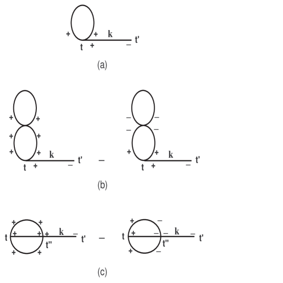
FIG. 1.: The Feynman diagrams contribute to the quantum kinetic equation for a self-interacting scalar theory up to two loops order. The tadpole contributions, (a) and (b), are canceled by a proper choice of $\Delta$.

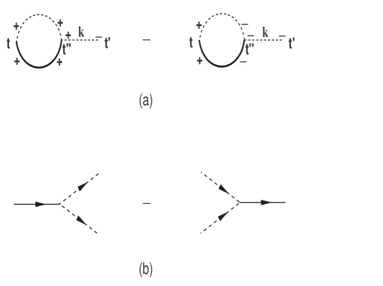
FIG. 2.: (a) The Feynman diagrams that contribute to the quantum kinetic equation for the pion distribution function. The solid line is the sigma meson propagator and the dashed line is the pion propagator. (b) The only contribution on-shell is the decay of a sigma meson into two pions minus the reverse process.

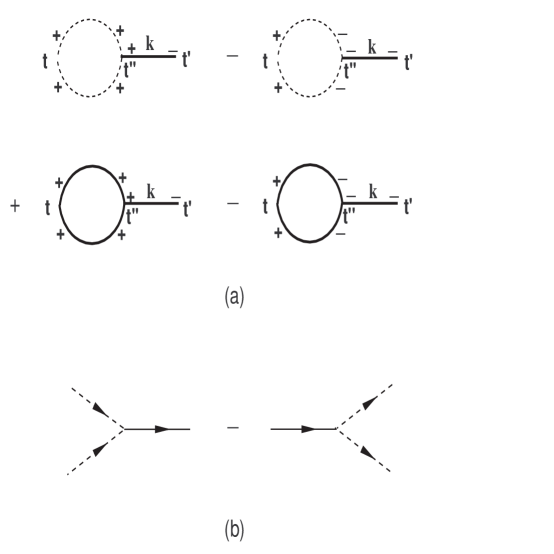
FIG. 3.: (a) The Feynman diagrams that contribute to the quantum kinetic equation for the sigma meson distribution function. The solid line is the sigma meson propagator and the dashed line is the pion propagator. (b) The only contribution on-shell is recombination of two pions into a sigma meson minus the decay of a sigma meson into two pions.

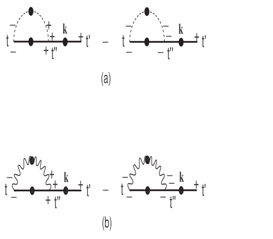
FIG. 4.: The Feynman diagrams that contribute to the quantum kinetic equation for the charged scalar distribution function to lowest order in $e^{2}$. The dashed and wavy lines are the HTL resummed longitudinal transverse photon propagators respectively, and the solid line is the HTL resummed scalar propagator. (a) Contribution from longitudinal photons. (b) Contribution from transverse photons.

REFERENCES

- [1] J.W. Harris and B. Muller, Annu. Rev. Nucl. Part. Sci. 46, 71 (1996); B. Muller in Particle Production in Highly Excited Matter, edited by H.H. Gutbrod and J. Rafelski, NATO ASI series B, vol. 303 (1993); H. Elze and U. Heinz, Phys. Rep. 183, 81 (1989); H. Meyer-Ortmanns, Rev. Mod. Phys. 68, 473 (1996); H. Satz, in Proceedings of the Large Hadron Collider Workshop, edited by G. Jarlskog and D. Rein (CERN, Geneva), Vol. 1, page 188; and in Particle Production in Highly Excited Matter, edited by H.H. Gutbrod and J. Rafelski, NATO ASI series B, Vol. 303 (1993).
- [2] B. Muller, The Physics of the Quark-Gluon Plasma, Lecture Notes in Physics, Vol. 225 (Springer-Verlag, Berlin, Heidelberg, 1985); L.P. Csernai, Introduction to Relativistic Heavy Ion Collisions (John Wiley and Sons, England, 1994); C.Y. Wong, Introduction to High-Energy Heavy Ion Collisions (World Scientific, Singapore, 1994).
- [3] K. Geiger, Phys. Rep. 258, 237 (1995); Phys. Rev. D54, 949 (1996); Phys. Rev. D56, 2665 (1996); Phys. Rev. D46, 4965 (1992); Phys. Rev. D47, 133 (1993); Quark-Gluon Plasma 2, edited by R.C. Hwa (World Scientific, Singapore, 1995).
- [4] H.-T. Elze and U. Heinz, in Quark-Gluon Plasma edited by R.C. Hwa (World Scientific, Singapore, 1990); H.-T. Elze and U. Heinz, Phys. Rep. 183, 81 (1989).
- [5] S. Mrówczyński, in Quark-Gluon Plasma [4]; S. Mrówczyński and P. Danielewicz, Nucl. Phys. B342, 345 (1990); S. Mrówczyński and U. Heinz, Ann. Phys. (N.Y.) 229, 1 (1994); S. Mrówczyński, hep-ph/9805435.
- [6] S.A. Bass et. al., Prog. Part. Nucl. Phys. 41 225 (1998).
- [7] I.D. Lawrie and D.B. McKernan, Phys. Rev. D55 2290 (1997); I.D. Lawrie, J. Phys. A21, L823 (1988); Phys. Rev. D40, 3330 (1989); Can. J. Phys. 71, 262 (1993).
- [8] D. Boyanovsky, I.D. Lawrie, and D.-S. Lee, Phys. Rev. D54, 4013 (1996).
- [9] F.T. Brandt, J. Frenkel, A. Guerra, Int. J. Mod. Phys. A13, 4281 (1998).
- [10] J. Rau and B. Muller, Phys. Rept. 272, 1 (1996).
- [11] X.-N. Wang, Phys. Rep. 280, 287 (1997).
- [12] K.J. Eskola, Prog. Theor. Phys. Suppl. 129, 1 (1997); K.J. Eskola, K. Kajantie, P.V. Ruuskanen, Eur. Phys. J. C1 627 (1998); K.J. Eskola, B. M ller, X.-N. Wang, Phys. Lett. B374, 20 (1996); K. J. Eskola, Nucl. Phys. A590, 383c (1995).
- [13] G. Aarts and J. Smit, Nucl. Phys. B555, 355 (1999); hep-ph/9906538; hep-ph/9909040.
- [14] A. Krasnitz and R. Venugopalan, hep-ph/9909203; hep-ph/9905319; hep-ph/9809433; hep-ph/9808332; hep-ph/9706329; R. Venugopalan, hep-ph/9907209.
- [15] A. Rajantie and M. Hindmarsh, hep-ph/9904270.
- [16] W. Poeschl and B. Mueller, nucl-th/9812066; hep-ph/9811441.
- [17] S. Jeon and L. Yaffe, Phys. Rev. D53, 5799 (1996); S. Jeon, Phys. Rev. D52, 3591 (1995).
- [18] D. Bodeker, hep-ph/9903478; Phys. Lett. B426, 351 (1998).
- [19] P. Arnold, D.T. Son and L.G. Yaffe, Phys. Rev. D59, 105020 (1999).
- [20] J.-P. Blaizot and E. Iancu, hep-ph/9903389; hep-ph/9906485.
- [21] M.A. Valle Basagoiti, hep-ph/9903462.
- [22] D.F. Litim and C. Manuel, hep-ph/9906210.
- [23] P. Danielewicz, Ann. Phys. (N.Y.) 152, 239 (1984).
- [24] D. Boyanovsky, H.J. de Vega, R. Holman, and M. Simionato, Phys. Rev. D60, 065003 (1999); D. Boyanovsky and H.J. de Vega, Phys. Rev. D59, 105019 (1999).
- [25] J.-P. Blaizot and E. Iancu, Phys. Rev. Lett. 76, 3080 (1996); Phys. Rev. D55, 973 (1997); ibid. 56, 7877 (1997). K. Takashiba, Int. J. Mod. Phys A 11, 2309 (1996).
- [26] R.D. Pisarski, Phys. Rev. Lett. 63, 1129 (1989); Phys. Rev. D47,5589 (1993).
- [27] E. Braaten and R.D. Pisarski, Nucl. Phys. B337, 569 (1990); ibid. B339, 310 (1990).
- [28] R.D. Pisarski, Physica A 158, 146 (1989); Phys. Rev. Lett. 63, 1129 (1989); Nucl. Phys. A525, 175 (1991).
- [29] R.D. Pisarski, Nucl. Phys. B309, 476 (1988).
- [30] N.P. Landsmann and C.G. van Weert, Phys. Rep. 145, 141 (1987).
- [31] T. Altherr and D. Seibert, Phys. Lett. B333, 149 (1994); T. Altherr, Phys. Lett. B341, 325 (1995).
- [32] T. Hatsuda, T. Kunihiro, and H. Shimizu, Phys. Rev. Lett. 82 2840 (1999); S. Chiku and T. Hatsuda, Phys. Rev. D58 076001 (1998); ibid. Phys. Rev. D57, 6 (1998).
- [33] U. Kraemmer, A. Rebhan, and H. Schulz, Ann. Phys. (N.Y.) 238, 286 (1995).
- [34] M.H. Thoma and C.T. Traxler, Phys. Lett. B378, 233 (1996).
- [35] D. Boyanovsky, H.J. de Vega, R. Holman, S.P. Kumar, and R.D. Pisarski, Phys. Rev. D58, 125009 (1998).
- [36] S. Leupold and M.H. Thoma, hep-ph/9908460.
- [37] J. Schwinger, J. Math. Phys. 2, 407 (1961).
- [38] K.T. Mahanthappa, Phys. Rev. 126, 329 (1962); P.M. Bakshi and K.T. Mahanthappa, J. Math. Phys. 41, 12 (1963).
- [39] L.V. Keldysh, JETP 20, 1018 (1965).
- [40] K.-C. Chou, Z.-B. Su, B.-L. Hao, and L. Yu, Phys. Rep. 118, 1 (1985).
- [41] D. Boyanovsky, H.J. de Vega and R. Holman, in Proceedings of the Second Paris Cosmology Colloquium, Observatoire de Paris, 1994, edited by H.J. de Vega and N. Sánchez (World Scientific, Singapore 1995), pp. 127-215; in Advances in Astrofundamental Physics, Erice Chalonge School, edited by N. Sánchez and A. Zichichi (World Scientific, Singapore 1995); D. Boyanovsky, H.J. de Vega, R. Holman, D.-S. Lee and A. Singh, Phys. Rev. D51, 4419 (1995); D. Boyanovsky, H.J. de Vega, R. Holman and J. Salgado, Phys. Rev. D54, 7570 (1996).
- [42] D. Boyanovsky, H.J. de Vega and R. Holman, in Current Topics in Astrofundamental Physics, Vth Erice Chalonge School, edited by N. Sánchez and A. Zichichi (World Scientific, Singapore 1996), pp. 183-270; D. Boyanovsky, H.J. de Vega, R. Holman and D.-S. Lee, Phys. Rev. D52, 6805 (1995); D. Boyanovsky, M. D’Attanasio, H.J. de Vega and R. Holman, Phys. Rev. D54, 1748 (1996).
- [43] M. Le Bellac, Thermal Field Theory (Cambridge University Press, Cambridge, England, 1996).
- [44] R.R. Parwani, Phys. Rev. D45, 4695 (1992).
- [45] L. Dolan and R. Jackiw, Phys. Rev. D9, 332 (1974).
- [46] P. Elmfors, K. Enqvist, and I. Vilja, Nucl. Phys. B422[FS], 521 (1994).
- [47] L.-Y. Chen, N. Goldenfeld and Y. Oono, Phys. Rev. Lett. 73, 1311 (1994); Phys. Rev.E54, 376 (1996).
- [48] T. Kunihiro, Prog. Theor. Phys. 95, 503 (1995); ibid. 97, 179 (1997); S. Ei, K. Fujii and T. Kunihiro, hep-th/9905088.
- [49] H.J. de Vega and J.F.J. Salgado, Phys. Rev. D56 6524, (1997).
- [50] I.L. Egusquiza and M.A. Valle-Basagoiti, hep-th/9611143; T. Kunihiro, Prog. Theor. Phys. Suppl. 131, 459 (1998).
- [51] V.E. Zakharov, V.S. Lv́ov, G. Falkovich, Kolmogorov Spectra of Turbulence I (Springer-Verlag, Berlin Heidelberg, 1992).
- [52] A. Bochkarev and J. Kapusta, Phys. Rev. D54, 4066 (1996).
- [53] D. Boyanovsky, H.J. de Vega, D.-S. Lee, Y.J. Ng, and S.-Y. Wang, Phys. Rev. D59, 105001 (1999); S.-Y. Wang, D. Boyanovsky, H.J. de Vega, D.-S. Lee, and Y.J. Ng, hep-ph/9902218.
- [54] R.D. Pisarski and M. Tytgat, Phys. Rev. D54, 2989 (1996).
- [55] A. Jakovac, A. Patkos, P. Petreczky, Zs. Szep, hep-ph/9905439. The authors thank A. Patkos for illuminating correspondence on these issues.
- [56] B.D. Serot and J.D. Walecka, Adv. Nucl. Phys. 16, 1 (1986).
- [57] D.H. Rischke, Phys. Rev. C58, 2331 (1998).
- [58] L.P. Csernai, P.J. Ellis, S. Jeon, and J.I. Kapusta, nucl-th/9908020.
- [59] D. Boyanovsky, H.J. de Vega, D.-S. Lee, and S.-Y. Wang (work in progress).
- [60] T. Altherr, Phys. Lett. B341, 325 (1995).
- [61] I. Dadic, Phys. Rev. D59, 125012 (1999).
- [62] P.F. Bedaque, Phys. Lett. B344, 23 (1995).
- [63] A. Niégawa, Phys. Lett. B416, 137 (1998).
- [64] A. Niégawa, hep-th/9905090.
- [65] C. Greiner and S. Leupold, Eur. Phys. J. C8, 517 (1999).
- [66] M.E. Carrington, H. Defu and M. Thoma, Eur. Phys. J. C7, 347 (1999).
- [67] D. Boyanovsky, D. Brahm, R. Holman and D.-S. Lee, Phys. Rev. D54, 1763 (1996).
- [68] L. Faddeev and A. Slavnov, Gauge Fields: An Introduction to Quantum Theory (Addison-Wesley, Redwood City, CA, 1991).
- [69] K. James and P.V. Landshoff, Phys. Lett. B251, 167 (1990).
- [70] The original method is due to Dirac: P.A.M. Dirac, Lectures in Quantum Mechanics (Yeshiva University, New York, 1964). See also: B. Hatfield, Quantum Field Theory of Point Particles and Strings (Addison Wesley, Redwood City, 1992); A. Hansson, T. Regge, and C. Teitelboim, Constrained Hamiltonian Systems (Academia Nazionale dei Lincei, Rome, 1976); M. Henneaux and C. Teitelboim, Quantization of Gauge Systems (Princeton University Press, 1992), and references therein.