The QCD description of diffractive processes

Abstract

We review the application of perturbative QCD to diffractive processes. We introduce the two gluon exchange model to describe diffractive $q\bar{q}$ and $q\bar{q}g$ production in deep inelastic scattering. We study the triple Regge limit and briefly consider multiple gluon exchange. We discuss diffractive vector meson production at HERA both at $t=0$ and large $|t|$. We demonstrate the non-factorization of diffractive processes at hadron colliders.

• University of Durham, Department of Physics, Durham DH1 3LE, UK

1 Introduction

Diffractive scattering has become a vast area of study in particle physics and generated a wide range of theoretical approaches. Here we will concentrate on those processes which have the potential to provide a deeper insight into the dynamics of strong interactions, that is into quantum chromodynamics (QCD). Our main focus will be on diffractive deep inelastic scattering. Diffraction in $p\bar{p}$-scattering or photoproduction will be discussed fairly briefly. The motivation for studying diffractive deep inelastic scattering is not only driven by the fact that we have excellent data, but also that it offers an opportunity to explore the interesting transition from “hard” to “soft” physics. Hard physics is associated with the well established parton picture and perturbative QCD, and is applicable to processes for which a large scale is present. Soft dynamics on the other hand, associated for example with total cross sections and elastic scattering of hadrons, is described by non-perturbative aspects of QCD. Diffractive deep inelastic scattering offers the opportunity to directly probe the semihard transition region and to link the, otherwise distinct, regimes of soft and hard physics. The means by which we attack the problem is perturbative QCD carefully extrapolated into the semihard regime. It is thus natural to put strong emphasis on diffractive processes, which are believed to be purely perturbative, such as diffractive vector meson production in deep inelastic scattering or in photoproduction when the momentum transfer is large.

The classical definition of diffraction in hadron-hadron or (virtual) photon-hadron scattering is the quasi elastic scattering of one hadron combined with the dissociation of the second hadron or photon. For example, at the electron-proton collider HERA, diffractive deep inelastic scattering is usually written

$$\gamma^{*}+p\mskip 5.0mu plus 5.0mu\rightarrow\mskip 5.0mu plus 5.0muX+Y$$ (1)

where $Y$ denotes the elastically scattered proton (or one of its low mass excitations) and $X$ denotes all the hadrons coming from the dissociating virtual photon. The classical method of detection is to tag the elastically scattered hadron. In the present high energy collider experiments, however, the elastically scattered protons usually disappear into the beampipe requiring special detectors far down, and adjacent to, the beampipe for their detection. Very often these detectors cannot deliver high enough statistics or good enough energy resolution so that an alternative method, the rapidity gap method, is employed. The rapidity gap method is based on the simple fact that the elastically scattered proton (or $Y$ state) travels in roughly the same direction as the original hadron leaving a large gap between the rapidity of this particle and the other outgoing hadrons forming the inclusive state $X$. Rapidity is a measure of the component of a particle’s velocity along the incoming proton direction. That is diffraction at the HERA electron-proton collider is characterized by the quasi-elastic scattering of the proton and the dissociation of the virtual photon. Such a diffractive event is in contrast to the usual deep inelastic scattering event

$$\gamma^{*}+p\mskip 5.0mu plus 5.0mu\rightarrow\mskip 5.0mu plus 5.0muX$$ (2)

in which the virtual photon breaks up the proton and the outgoing hadrons populate the full interval of rapidity. Nevertheless about 10% of all events in deep inelastic scattering are of diffractive nature and high statistics data samples have been collected at HERA [2].

Before this diffraction was observed in hadron collisions and is still being measured at the Tevatron proton-antiproton collider at the present time. The relative rate of diffraction compared to the total rate is on a similar level to that of deep inelastic scattering [3]. The problem, however, is that the total cross section is huge and only a tiny fraction of events are of special interest such as heavy particles ($W$ and $Z$ bosons or the top quark) and jets of high transverse momentum. Since the hadronic activity is much higher in hadron-hadron scattering compared to deep inelastic scattering the detection of rapidity gaps is a tedious task. With a trigger set on $W$ bosons or high-$p_{T}$ jets the fraction of events with a rapidity gap is only on the level of 1% [4]. It requires a special effort to extract diffractive processes at the Tevatron whereas at HERA they almost come for free.

There is a group of processes which do not precisely belong to diffraction in the way we have defined it. These are processes with large momentum transfer across the rapidity gap. Examples are the production of opposite di-jets with a rapidity gap in between them at the Tevatron, or diffractive vector meson production at HERA. Due to the large momentum transfer the proton (or antiproton) always breaks up. Because of the large rapidity gap, however, they are closely related to the traditional diffractive processes.

Figure 1: Diagrams for DIS, $\gamma^{*}p\rightarrow X$, and inclusive diffractive DIS, $\gamma^{*}p\rightarrow Xp$. In the latter process there is a rapidity gap between the outgoing hadrons $X$ and the slightly deflected proton. In the diagram the gap has been associated with Pomeron exchange carrying a fraction $x_{I\!\!P}$ of the proton’s momentum.

The early attempts to describe diffractive scattering were based on Regge phenomenology where the Pomeron is thought to be the leading Regge pole with a well defined and unique, process-independent Regge trajectory. The Pomeron trajectory, together with secondary trajectories, allows one to fit all kinds of hadronic data (total and elastic cross sections) [1]. These universal trajectories $\alpha_{R}(t)$ form the backbone of Regge phenomenology. According to early analyses it seemed that diffraction can be described in terms of triple Regge diagrams (see Section 3) without changing the trajectories or the couplings to hadrons. The only free parameters were the couplings of the Reggeons amongst themselves. The more recent results [3] from the Tevatron, however, indicate that this simple picture does not hold at very high energies. The extrapolation of the cross section from the Sp$\bar{\rm p}$S CERN collider energy to the Tevatron energy clearly overshoots the data. The explanation for the discrepancy is most likely given by unitarity corrections.

After introducing the structure functions that can be measured in diffractive deep inelastic scattering, we outline in Section 3 the Regge description of diffractive processes based on the Pomeron, or the “soft” Pomeron as it is now frequently called. The perturbative QCD description of diffractive processes, which is the subject of this review, is based on two gluon exchange. This will form the framework of our discussions from Section 4 onwards. Two gluon exchange is the simplest form of vacuum quantum exchange and, for historical reasons, people often speak of the “hard” Pomeron. However the connection between “soft” (non-perturbative) and “hard” (perturbative) diffraction is far from clear. The different energy behaviours are very evident, as will be seen, for example, when we discuss diffractive vector meson photo- and electro-production (see, in particular, Fig. 9).

2 Diffractive structure functions

First let us recall (inclusive) deep inelastic electron-proton scattering, $ep\rightarrow eX$, where $X$ represents all the fragments of the proton which has been broken up by the high energy electron. The basic subprocess $\gamma^{*}p\rightarrow X$ is shown in Fig. 1(a). It can be expressed in terms of two functions $F_{2}$ and $F_{L}$ which characterize the structure of the proton. These proton structure functions depend on two (invariant) variables, the “virtuality” of the photon $Q^{2}\equiv-q^{2}$ and the Bjorken $x$-variable

$$x\mskip 5.0mu plus 5.0mu\equiv\mskip 5.0mu plus 5.0mu\frac{Q^{2}}{2p.q}\mskip 5.0mu plus 5.0mu=\mskip 5.0mu plus 5.0mu\frac{Q^{2}}{Q^{2}+W^{2}},$$ (3)

where $p$ and $q$ are the four-momenta of the proton and virtual photon respectively, see Fig. 1(a). $W$ is the total $\gamma^{*}p$ centre-of-mass energy. If we were to view the proton as made up of massless, point-like quark constituents, then it is easy to show that $x$ is the fraction of the proton’s momentum carried by the quark struck by the virtual photon. In this simple quark model $F_{L}=0$ and

$$F_{2}\mskip 5.0mu plus 5.0mu=\mskip 5.0mu plus 5.0muF_{T}\mskip 5.0mu plus 5.0mu=\mskip 5.0mu plus 5.0mu\sum_{q}\>e_{q}^{2}\>xq(x)$$ (4)

is independent of $Q^{2}$. The sum is over the flavours of quarks, with electric charge $e_{q}$ (in units of $e$) and distributions $q(x)$. $F_{T,L}$ are the proton structure functions for DIS by transversely, longitudinally polarised photons.

The general form of the DIS cross section, up to target mass corrections, is

$$\frac{d^{2}\sigma(ep\rightarrow eX)}{dxdQ^{2}}\mskip 5.0mu plus 5.0mu=\mskip 5.0mu plus 5.0mu\frac{2\pi\alpha^{2}}{xQ^{4}}\>\left\{[1+(1-y)^{2}]\>F_{2}(x,Q^{2})\>-\>y^{2}F_{L}(x,Q^{2})\right\}$$ (5)

where $\alpha$ is the electromagnetic coupling. The third variable $y$ is needed to fully characterize the DIS process, $ep\rightarrow eX$, namely $y=Q^{2}/xs$ where $\sqrt{s}$ is the total centre-of-mass energy of the electron-proton collision.

Now we turn to inclusive diffractive DIS, $ep\rightarrow eXp$, for which the subprocess is $\gamma^{*}p\rightarrow Xp$, where a slightly deflected proton and the cluster $X$ of outgoing hadrons are well separated in rapidity. In terms of Regge terminology the rapidity gap is associated with Pomeron (or vacuum quantum number) exchange, shown by the zig-zag line in Fig. 1(b). The $\gamma^{*}p\rightarrow Xp$ subprocess is described by diffractive structure functions $F_{2,L}^{D}$, which now depend on four variables: $\beta\equiv x/x_{I\!\!P}$, $Q^{2}$, $x_{I\!\!P}$ and $t$. The variable $x_{I\!\!P}$ is the fraction of the proton’s momentum that is carried away by the Pomeron. The variable $\beta$ in diffractive DIS plays an analogous role to $x$ in DIS

$$\beta\mskip 5.0mu plus 5.0mu\equiv\mskip 5.0mu plus 5.0mu\frac{x}{x_{I\!\!P}}\mskip 5.0mu plus 5.0mu=\mskip 5.0mu plus 5.0mu\frac{Q^{2}}{2x_{I\!\!P}p.q}\mskip 5.0mu plus 5.0mu=\mskip 5.0mu plus 5.0mu\frac{Q^{2}}{Q^{2}+M^{2}}$$ (6)

where $M$ is the invariant mass of the diffractively produced $X$ cluster in Fig. 1(b).

In analogy to (5), the general form of the diffractive DIS cross section is

$$\frac{d^{4}\sigma^{D}(ep\rightarrow eXp)}{d\beta dQ^{2}dx_{I\!\!P}dt} = \frac{2\pi\alpha^{2}}{\beta Q^{4}}\left\{[1+(1-y)^{2}]\>F_{2}^{D(4)}(\beta,Q^{2},x_{I\!\!P},t)\right.$$ (7)

$$-y^{2}\left.F_{L}^{D(4)}(\beta,Q^{2},x_{I\!\!P},t)\right\}.$$

The superscript (4) is to indicate that the structure functions depend on four independent variables. The $F_{L}$ contribution is often neglected due to the smallness of $y^{2}$ in most of the measurements. The variable $t=(p-p^{\prime})^{2}$ is the square of the 4-momentum carried by the Pomeron. Most diffractive DIS events occur for small values of $t$. Usually $t$ is integrated over and measurements of the structure function

$$F_{2}^{D(3)}(\beta,Q^{2},x_{I\!\!P})\mskip 5.0mu plus 5.0mu=\mskip 5.0mu plus 5.0mu\int\>dt\>F_{2}^{D(4)}(\beta,Q^{2},x_{I\!\!P},t)$$ (8)

are made.

3 Regge approach to diffraction

The early attempts to describe diffractive scattering were based on Regge theory (see, for example, [5]), in which the basic idea is that sequences of hadrons of mass $m_{i}$ and spin $j_{i}$ lie on Regge trajectories $\alpha(t)$ such that $\alpha(m_{i}^{2})=j_{i}$. Prior to QCD, strong interactions were thought to be due to the exchange of complete trajectories of particles. Indeed the Regge model is able to successfully describe all kinds of “soft” high energy hadronic scattering data: differential, elastic and total cross section measurements. In this model the high energy behaviour of a hadron scattering amplitude at small angles has the form

$$A(s,t)\mskip 5.0mu plus 5.0mu\sim\mskip 5.0mu plus 5.0mu\sum_{R}\>\beta(t)\>s^{\alpha_{R}(t)}$$ (9)

where for simplicity we have omitted the signature factor. $s$ is the square of the centre-of-mass energy and $-t$ is the square of the four-momentum transfer. The observed hadrons were found to lie on trajectories $\alpha_{R}(t)$ which are approximately linear in $t$ and parallel to each other. That is hadrons of increasing spin and mass, but with the other quantum numbers the same, lie on a single trajectory $\alpha_{R}(t)$. The leading such trajectories are the $\rho,a_{2},\omega$ and $f$ trajectories which are all approximately degenerate with

$$\alpha_{R}(t)\mskip 5.0mu plus 5.0mu\simeq\mskip 5.0mu plus 5.0mu0.5\>+\>0.9t.$$ (10)

For example only the $\rho$ trajectory has the appropriate quantum numbers to be exchanged in the process $\pi^{-}p\rightarrow\pi^{0}n$. The energy or $s$ dependence of the differential cross section $d\sigma/dt$ therefore determines $\alpha_{\rho}(t)$ for $t<0$, see (9). For small $|t|$ the trajectory $\alpha_{\rho}(t)$ is found to be linear in $t$ and, when extrapolated to positive $t$, to pass through the $\rho(1^{-})$ and $\rho(3^{-})\ldots$ states, i.e. $\alpha_{\rho}(m_{\rho}^{2})=1,3,\ldots$ at the appropriate mass values.

So far so good, but the total cross sections are observed to increase slowly with energy at high energies, so we need a higher lying trajectory. This is best seen from the optical theorem which expresses a total cross section (say, for $AB\rightarrow X$) in terms of the imaginary part of the forward ($AB\rightarrow AB$) elastic scattering amplitude

$$\sigma(AB\rightarrow X)\mskip 5.0mu plus 5.0mu=\mskip 5.0mu plus 5.0mu\frac{1}{s}{\rm Im}A(s,0)\mskip 5.0mu plus 5.0mu=\mskip 5.0mu plus 5.0mu\sum_{R}\>\beta_{R}\>s^{\alpha_{R}(0)-1}.$$ (11)

To account for the asymptotic energy dependence of the total cross sections a Pomeron (or vacuum quantum number exchange) trajectory is invoked with intercept $\alpha_{I\!\!P}(0)\sim 1.08$. Indeed the total, elastic and differential hadronic cross section data are found to be well described (for small $|t|$) by taking a universal pole form for the Pomeron

$$\alpha_{I\!\!P}(t)\mskip 5.0mu plus 5.0mu\simeq\mskip 5.0mu plus 5.0mu1.08\>+\>0.25t,$$ (12)

together with the other sub-leading trajectories as in (10) [1]. The Pomeron should be regarded as an effective trajectory, since the $s^{0.08}$ power behaviour of the total cross sections will ultimately violate the Froissart bound. The link between this successful Regge description of “soft” processes and the underlying fundamental theory of QCD is not, as yet, known in detail. Most probably Pomeron exchange originates mainly from the exchange of a two-gluon bound state, while the meson trajectories $(\rho,a_{2},\omega,f)$ correspond to $q\bar{q}$ bound states. The Regge Pomeron discussed above is now often called the “soft” Pomeron.

Figure 2: The DIS and diffractive DIS cross sections expressed symbolically as structure functions via the optical theorem and its generalisation. The Regge limits are shown in the rightmost diagrams (where the photon couples via a quark configuration). A summation over allowed Regge exchanges is implied in (b).

To apply this approach to inclusive DIS and, more especially to its diffractive component, we again make use of the optical theorem, together with its generalisation by Mueller [7], which are symbolically shown by the equalities in Fig. 2. The optical theorems express the total cross sections in terms of the imaginary parts of the 2-body (or 3-body) forward elastic scattering amplitudes, or to be precise the discontinuities of the amplitudes across the cuts along the $W^{2}$ (or $M^{2}$) axes, which are indicated by the dotted lines in Fig. 2(a) (or (b)). The last diagrams show the various Regge limits for the structure functions, where the coupling to the photon is via a quark line. For DIS this gives

$$F_{2}\>\sim\sum_{i}\beta_{i}(W^{2})^{\alpha_{i}(0)-1}\quad\sim\quad\sum_{i}\beta_{i}x^{1-\alpha_{i}(0)}$$ (13)

for small $x$, see (3). In the naive parton model the valence and sea quark contributions to $F_{2}$ are associated with meson and Pomeron exchange respectively, and so using (4) we have

$$xq_{V}\>\sim\>x^{1-\alpha_{R}(0)}\quad\sim\quad x^{0.5}$$

$$xq_{S}\>\sim\>x^{1-\alpha_{I\!\!P}(0)}\quad\sim\quad x^{-0.08}$$ (14)

for small $x$.

For diffractive DIS, $\gamma^{*}p\rightarrow Xp$, we apply Mueller’s generalisation of the optical theorem [7]. For this diffractive case, that is when $s/M^{2}$ is large, the theorem is shown pictorially by the first two diagrams of Fig. 2(b). That is the cross section is given by the discontinuity across the $M^{2}$ cut of the (three-body) $\gamma^{*}p\bar{p}$ elastic amplitude, where a sum over the exchange Reggeons is implied. The Regge prediction depends on whether $M^{2}$ is large or small. For small $M^{2}$ the quark box gives the main contribution to photon-Pomeron scattering. In Ref. [8] a charge conjugation $C=1$ vector current coupling of the Pomeron to quarks was introduced with a free coupling constant. The resulting contribution to diffraction due to the quark box diagram is found to be

$$F_{2}^{D}\mskip 5.0mu plus 5.0mu\sim\mskip 5.0mu plus 5.0mu\beta(1-\beta).$$ (15)

This model shows already many of the properties which are also present in the two gluon exchange approach [9] . It is important to note the leading twist nature of diffractive deep inelastic scattering, that is $F_{2}^{D}$ is independent of $Q^{2}$. One also finds the strong alignment of the quark-antiquark pair along the photon-Pomeron axis which is a consequence of the low transverse momentum $k_{t}$ of the quarks relative to this axis. The particular property of alignment has already been pointed out by Bjorken [10]. It was argued in Ref. [8] that the quark-Pomeron coupling for inclusive DIS and diffractive DIS should be the same and by fitting inclusive data one can extract the coupling constant and make predictions for diffraction. Indeed some 10% of HERA DIS events were predicted to be diffractive.

For large $M^{2}$, on the other hand, we have the double Regge limit ($s/M^{2}\rightarrow\infty$ and $M^{2}\rightarrow\infty$) and the diffractive structure function is described by a sum of triple Regge diagrams

$$F_{2}^{D}\>\sim\>\sum_{i,j,k}\beta_{ijk}\left(\frac{s}{M^{2}}\right)^{\alpha_{j}(t)+\alpha_{k}(t)}\>(M^{2})^{\alpha_{i}(0)}.$$ (16)

The leading behaviour, which is given by the triple Pomeron contribution, is

$$F_{2}^{D}\mskip 5.0mu plus 5.0mu\sim\mskip 5.0mu plus 5.0mu(M^{2})^{\alpha_{I\!\!P}(0)-2\alpha_{I\!\!P}(t)}\mskip 5.0mu plus 5.0mu\sim\mskip 5.0mu plus 5.0mu1/M^{2}.$$ (17)

4 Two-gluon exchange model of diffraction

We now use perturbative QCD to describe the diffractive DIS process $\gamma^{*}p\rightarrow Xp$. In QCD the “Pomeron” (or vacuum quantum number exchange) is, in its simplest form, represented by two gluons [11, 12]. The minimum number of gluons to form a colourless state is of course two. It is not excluded that more than two gluons are exchanged and it is important that whenever we talk about two-gluon exchange to remember there is the possibility to extend the formalism to multigluon exchange. One might object that the whole process is soft and perturbation theory not applicable. Saturation effects for high parton densities, however, screen soft contributions, so that a fairly large fraction of the cross section is hard and therefore eligible for a perturbative treatment [13].

The two basic pQCD diagrams are shown in Fig. 3, in which the photon dissociates into either a $q\bar{q}$ pair or $q\bar{q}g$. In the first diagram the $q$ and $\bar{q}$ carry fractions $\alpha$ and $(1-\alpha)$ of the momentum of the photon, and have transverse momenta $\pm\mbox{\boldmath$k$}_{t}$. In the second diagram these variables apply to the gluon and the $(q\bar{q})$ system. At first sight it might appear that $q\bar{q}g$ would be a small correction to $q\bar{q}$ production on account of an extra $\alpha_{S}$ factor. However $q\bar{q}g$ production dominates at large $M^{2}$. It incorporates an extra $t$-channel spin 1 gluon in contrast to the (lower lying) $t$-channel spin $\frac{1}{2}$ quark exchange of $q\bar{q}$ production. In fact $q\bar{q}g$ is described by the triple Pomeron diagram and gives the leading contribution at large $M^{2}$ (or small $\beta$), whereas $q\bar{q}$ production is leading at small $M^{2}$, see Fig. 2(b).

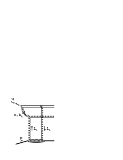
Figure 3: Diffractive $q\bar{q}$ and $q\bar{q}g$ electroproduction mediated by the exchange of two gluons with transverse momenta $\pm{\bf\ell}_{t}$. We view the photon as dissociating into either a quark dipole or an effective gluon dipole, made up of a gluon and a compact $q\bar{q}$ pair.

The intuitive picture is as follows. In the target (proton) restframe the photon dissociates into a $q\bar{q}$-pair far upstream the target. The $q\bar{q}$-pair may radiate a gluon, and the whole parton configuration scatters quasi-elastically off the proton via a two-gluon exchange. The timescale on which the fluctuation occurs is proportional to $1/(x\mskip 5.0mu plus 5.0mum_{p})$ where $m_{p}$ is the proton rest mass. At very small $x$ the fluctuation is long lived whereas the scattering is a sudden short impact of the $q\bar{q}$-pair or the $q\bar{q}g$-final state on the target. The impact changes the virtual into a real state but it does not change the position in impact parameter space which can be viewed as being frozen during the scattering.

It is informative to show why the fluctuation and interaction timescales are so different. For this it is convenient to use light-cone perturbation theory (see, for example, [14]) and to express the particle four momenta in the form

$$k_{\mu}\mskip 5.0mu plus 5.0mu=\mskip 5.0mu plus 5.0mu(k_{+},k_{-},\mbox{\boldmath$k$}_{t})$$ (18)

where $k_{\pm}=k_{0}\pm k_{3}$. In this approach all the particles are on mass-shell

$$k^{2}=k_{+}k_{-}\>-\>k_{t}^{2}\mskip 5.0mu plus 5.0mu=\mskip 5.0mu plus 5.0mum^{2},$$ (19)

and $k_{+}$ and $\mbox{\boldmath$k$}_{t}$ are conserved at each vertex. In the proton rest frame we have

$$p_{\mu}\mskip 5.0mu plus 5.0mu=\mskip 5.0mu plus 5.0mu(m_{p},m_{p},\mbox{\boldmath$0$}),\quad\quad\quad q_{\mu}\mskip 5.0mu plus 5.0mu=\mskip 5.0mu plus 5.0mu(q_{+},\>-Q^{2}/q_{+},\>\mbox{\boldmath$0$}),$$

$$k_{\mu}\mskip 5.0mu plus 5.0mu=\mskip 5.0mu plus 5.0mu(k_{+},\>m_{T}^{2}/k_{+},\>\mbox{\boldmath$k$}_{t}),\quad\quad\quad \ell_{\mu}\mskip 5.0mu plus 5.0mu=\mskip 5.0mu plus 5.0mu(\ell_{+},\>\ell_{t}^{2}/\ell_{+},\>\mbox{\boldmath$\ell$}_{t}),$$

with $m_{T}^{2}=m^{2}+k_{t}^{2}$ where $m$ is the mass of the quark. According to the uncertainty principle the $\gamma^{*}\rightarrow q\bar{q}$ fluctuation time

$$\tau_{\gamma}\>\sim\>\frac{1}{\Delta E}\mskip 5.0mu plus 5.0mu=\mskip 5.0mu plus 5.0mu\left|\frac{2}{q_{-}-k_{1-}-k_{2-}}\right|\mskip 5.0mu plus 5.0mu=\mskip 5.0mu plus 5.0mu\frac{2q_{+}}{Q^{2}+m_{T}^{2}/\alpha+m_{T}^{2}/(1-\alpha)}\>\simeq\>\frac{2q_{+}}{Q^{2}}\mskip 5.0mu plus 5.0mu=\mskip 5.0mu plus 5.0mu\frac{1}{m_{p}x}$$ (21)

at high $Q^{2}$, where $k_{1}$ and $k_{2}$ are the four momenta of the quark and antiquark. The momentum fractions, shown in Fig. 3, are $\alpha=k_{1+}/q_{+}$ and $1-\alpha=k_{2+}/q_{+}$. The factor 2 in (21) occurs because the energy $k_{0}=(k_{+}+k_{-})/2$. An estimate of the interaction time can be obtained from the typical time for the emission of a gluon of momentum $\ell$ from the quark $k_{1}$, say. Then

$$\tau_{i}\>\sim\>\left|\frac{2}{k_{1-}-k_{1-}^{\prime}-\ell_{-}}\right|\mskip 5.0mu plus 5.0mu=\mskip 5.0mu plus 5.0mu\left|\frac{2q_{+}}{m_{T}^{2}/\alpha-m_{T}^{2}/\alpha^{\prime}-\ell_{t}^{2}/(\alpha-\alpha^{\prime})}\right|\>\simeq\>\frac{2\ell_{+}}{\ell_{t}^{2}}\mskip 5.0mu plus 5.0mu=\mskip 5.0mu plus 5.0mu\frac{1}{m_{p}x_{\ell}}$$ (22)

since $\alpha-\alpha^{\prime}=\ell_{+}/q_{+}$ and $\alpha^{\prime}=k_{1+}^{\prime}/q_{+}$. We can regard $x_{\ell}$ as the Bjorken variable for the gluon-proton interaction. We are concerned with the kinematic region $x\ll x_{\ell}$ where the leading $\log(x_{\ell}/x)$ approximation is appropriate, and so we have $\tau_{\gamma}\gg\tau_{i}$.

One should note that the above picture is valid in a certain frame in combination with a certain physical gauge condition, $p\cdot A=0$ ($p$ is the proton momentum and $A$ the gluon vector potential). In this gauge the parton shower evolves from the photon end while Bremsstrahlung from the proton is suppressed. One can turn to the Breit frame where the proton is fast moving and with it the Pomeron. The Pomeron in this frame is a long lived and very complicated virtual fluctuation. It is then more appropriate to use the gauge condition $q^{\prime}\cdot A=0$ ($q^{\prime}=q+xp$ is the corresponding light-cone vector in the photon direction) under which the parton shower evolves from the Pomeron end. The results do not change but the physical interpretation is less appealing.

The virtual fluctuation of the photon into a $q\bar{q}$-pair or a $q\bar{q}g$-final state is described by photon wave functions. The QCD-wave function for a $q\bar{q}$-pair has first been discussed in Refs. [15, 16]. Similar results have already been derived within QED. In Ref. [17] the fluctuation of a photon into a pair of muons has been studied as a model for deep inelastic scattering. The discussion of gluon radiation is a more recent development starting with Ref. [18].

The wave function for a $q\bar{q}$-pair depends on the polarization of the parent photon, whether it is transversely ($T$) or longitudinally ($L$) polarized. The key assumption in the whole approach is the eikonal-type coupling of the $t$ channel gluons with momentum $\ell$ to fast moving $s$ channel quarks and gluons such that

$$\langle p-\ell|\gamma^{\mu}|p\rangle\mskip 5.0mu plus 5.0mu\simeq\mskip 5.0mu plus 5.0mu2p^{\mu}$$ (23)

where $p$ and $p-\ell$ are the momenta of the fast incoming and outgoing partons. This approximation is correct at very high energies $(\ell\ll p)$. The derivation of the transverse and longitudinal wave functions, based on an explicit spinor representation, can be found in Ref. [19] or Ref. [20]. For a transversely polarized photon of, say, helicity $\lambda_{\gamma}=+1$ the wave functions $\Psi_{\lambda\lambda^{\prime}}$ are

$$\Psi_{+-}^{T} = \frac{\sqrt{2}e_{q}\alpha\mbox{\boldmath$k$}_{t}\cdot\mbox{\boldmath$\varepsilon$}(\lambda_{\gamma}=1)}{k_{t}^{2}+\alpha(1-\alpha)Q^{2}},$$

$$\Psi_{-+}^{T} = -\>\frac{\sqrt{2}e_{q}(1-\alpha)\mbox{\boldmath$k$}_{t}\cdot\mbox{\boldmath$\varepsilon$}(\lambda_{\gamma}=1)}{k_{t}^{2}+\alpha(1-\alpha)Q^{2}}$$

where $\varepsilon$ is the polarization vector of the virtual gluon, $\lambda,\lambda^{\prime}$ are the helicities of the quark, antiquark (with $\pm$ denoting helicity $\pm\frac{1}{2}$), and $e_{q}$ is the electric charge of the quark. The general structure of (4) is clear. For a massless quark, helicity conservation at a quark-photon vertex requires $\lambda\neq\lambda^{\prime}$. The momentum fractions $\alpha,(1-\alpha)$ appear in the numerator because the photon helicity tends to follow the fast quark, antiquark. Angular momentum conservation forbids collinear $q,\bar{q}$ production. Hence the $k_{t}$ factor signifying a $P$-wave interaction. Finally, the structure of the denominator has its origin in (21) with $m_{T}^{2}=k_{t}^{2}$. The longitudinal wave functions (with $\lambda_{\gamma}=0$) are found to be

$$\Psi_{+-}^{L}\mskip 5.0mu plus 5.0mu=\mskip 5.0mu plus 5.0mu\Psi_{-+}^{L}\mskip 5.0mu plus 5.0mu=\mskip 5.0mu plus 5.0mu\frac{2e_{q}\alpha(1-\alpha)Q}{k_{t}^{2}+\alpha(1-\alpha)Q^{2}}.$$ (25)

The effective wave function for the $q\bar{q}g$-state requires some remarks. Since the photon does not couple to gluons directly it cannot decay into a gluon dipole. At large $Q^{2}$, however, the colour structure of the $q\bar{q}$ effectively combines into that of a gluon leading to a gluon dipole. This feature is based on the strong ordering of the transverse momenta in the leading log($Q^{2}$) approximation to diffractive DIS, that is, it is valid when $k_{t}\ll Q$ and $\alpha\ll 1$, and when the photons are transversely polarized. The contribution due to the quark-box can be factorized (as becomes more explicit later on) and we are left with the following expression for the effective gluon dipole wave function describing the $\gamma^{*}\rightarrow(q\bar{q})g$ transition [21, 22]:

$$\Psi_{q\bar{q}g}\mskip 5.0mu plus 5.0mu=\mskip 5.0mu plus 5.0mu\frac{1}{\sqrt{\alpha Q^{2}}}\mskip 5.0mu plus 5.0mu\frac{k_{t}^{2}\mskip 5.0mu plus 5.0mu(\mbox{\boldmath$\varepsilon$}_{1}\cdot\mbox{\boldmath$\varepsilon$}_{2})\>-\>2(\mbox{\boldmath$k$}_{t}\cdot\mbox{\boldmath$\varepsilon$}_{1})(\mbox{\boldmath$k$}_{t}\cdot\mbox{\boldmath$\varepsilon$}_{2})}{k_{t}^{2}+\alpha Q^{2}},$$ (26)

where $\mbox{\boldmath$\varepsilon$}_{1}$ and $\mbox{\boldmath$\varepsilon$}_{2}$ are the polarization vectors of the $(q\bar{q})$ and $g$ forming the gluon dipole. Since $\alpha\ll 1$ we have replaced $(1-\alpha)$ by 1 in (26). Otherwise the wave function is to be interpreted in analogy to eqs. (4, 25).

In order to ensure gauge invariance we have to consider all possible couplings of the two $t$ channel gluons to the quark- or ‘gluon’-dipole. In total there are four configurations of which only one is shown in Fig. 3. This leads to the following expression

$$D\Psi(\mbox{\boldmath$k$}_{t},\mbox{\boldmath$\ell$}_{t}) = 2\mskip 5.0mu plus 5.0mu\Psi(\alpha,\mbox{\boldmath$k$}_{t})\mskip 5.0mu plus 5.0mu-\mskip 5.0mu plus 5.0mu\Psi(\alpha,\mbox{\boldmath$k$}_{t}+\mbox{\boldmath$\ell$}_{t})\mskip 5.0mu plus 5.0mu-\mskip 5.0mu plus 5.0mu\Psi(\alpha,\mbox{\boldmath$k$}_{t}-\mbox{\boldmath$\ell$}_{t})$$ (29)

$$\simeq \left\{\,\vbox{\openup 3.0pt\halign{\strut$\displaystyle{#}\hfil$&\tqs\rm#\hfil\cr-\mbox{\boldmath$\ell$}_{t}^{i}\mbox{\boldmath$\ell$}_{t}^{j}\mskip 5.0mu plus 5.0mu\frac{\partial^{2}\Psi(\alpha,\mbox{\boldmath$k$}_{t})}{\partial\mbox{\boldmath$k$}_{t}^{i}\partial\mbox{\boldmath$k$}_{t}^{j}}&\hskip 25.0pt\rm\mbox{for $\ell_{t}\ll k_{t}$}, \cr 2\mskip 5.0mu plus 5.0mu\Psi(\alpha,\mbox{\boldmath$k$}_{t})&\hskip 25.0pt\rm\mbox{for $\ell_{t}\gg k_{t}$}. \crcr}}\right.$$

The amplitude for diffractive scattering is basically obtained by folding $D\Psi$ with the unintegrated gluon distribution $\cal{F}$:

$$A^{D} \sim \int\frac{d^{2}\mbox{\boldmath$\ell$}_{t}}{\pi\mskip 5.0mu plus 5.0mu\ell_{t}^{2}}\mskip 5.0mu plus 5.0muD\Psi(\mbox{\boldmath$k$}_{t},\mbox{\boldmath$\ell$}_{t})\mskip 5.0mu plus 5.0mu\alpha_{S}(\ell_{t}^{2}){\cal F}(x_{I\!\!P},\ell_{t}^{2})\mskip 5.0mu plus 5.0mu\mskip 5.0mu plus 5.0mu.$$ (30)

The form for $A^{D}$ is an example of the so-called ‘$k_{t}$-factorization theorem’ [23], here applied to the transverse momentum $\ell_{t}$. The distribution ${\cal F}$, unintegrated over $\ell_{t}^{2}$,contains all the details of the coupling of the two $t$ channel gluons to the proton as indicated by the bubble in Fig. 3. This gluon distribution ${\cal F}(x,\ell_{t}^{2})$ is a universal function applicable to all hard scattering processes involving the proton and, indeed, the gluon is the dominant parton distribution at small $x$. Integrating ${\cal F}(x,\ell_{t}^{2})$ over $\ell_{t}^{2}$ gives the conventional gluon distribution $xg(x)$.

We have now, in principle, all the “QCD-based” ingredients to write down the diffractive cross section. Before we do that we comment on the role of the wave function for the $\beta$-spectrum. It has been demonstrated in Ref. [24] that the basic shape of the $\beta$-spectrum arises from the wave functions. It depends only weakly on the details of the unintegrated distribution $\cal{F}$. Looking back at (29) we see a ‘hard’ ($\ell_{t}\ll k_{t}$) and a ‘soft’ ($\ell_{t}\gg k_{t}$) limit for $D\Psi$. The typical scale for $\ell_{t}$ is given by the dynamics inside the proton. The hard limit is represented by the second derivative of the wave functions and the soft limit by the wave function itself. The second derivatives are

$$\delta^{ij}\mskip 5.0mu plus 5.0mu\frac{\partial^{2}\Psi^{T}_{+-}}{\partial\mbox{\boldmath$k$}_{t}^{i}\partial\mbox{\boldmath$k$}_{t}^{j}} = \alpha(1-\alpha)Q^{2}\mskip 5.0mu plus 5.0mu\frac{\sqrt{2}\mskip 5.0mu plus 5.0mue_{q}\mskip 5.0mu plus 5.0mu(1-\alpha)\mskip 5.0mu plus 5.0mu\mbox{\boldmath$k$}_{t}\cdot\mbox{\boldmath$\varepsilon$}(\lambda_{\gamma}=1)}{[k_{t}^{2}+\alpha(1-\alpha)Q^{2}]^{3}},$$ (31)

$$\delta^{ij}\mskip 5.0mu plus 5.0mu\frac{\partial^{2}\Psi^{L}_{+-}}{\partial\mbox{\boldmath$k$}_{t}^{i}\partial\mbox{\boldmath$k$}_{t}^{j}} = 4\mskip 5.0mu plus 5.0mue_{q}\mskip 5.0mu plus 5.0mu\alpha(1-\alpha)\mskip 5.0mu plus 5.0muQ\mskip 5.0mu plus 5.0mu\frac{k_{t}^{2}-\alpha(1-\alpha)Q^{2}}{[k_{t}^{2}+\alpha(1-\alpha)Q^{2}]^{3}},$$ (32)

$$\delta^{ij}\mskip 5.0mu plus 5.0mu\frac{\partial^{2}\Psi_{q\bar{q}g}}{\partial\mbox{\boldmath$k$}_{t}^{i}\partial\mbox{\boldmath$k$}_{t}^{j}} = \frac{k_{t}^{2}(\mbox{\boldmath$\varepsilon$}_{1}\cdot\mbox{\boldmath$\varepsilon$}_{2})\>-\>2(\mbox{\boldmath$k$}_{t}\cdot\mbox{\boldmath$\varepsilon$}_{1})(\mbox{\boldmath$k$}_{t}\cdot\mbox{\boldmath$\varepsilon$}_{2})}{\sqrt{\alpha Q^{2}}}\mskip 5.0mu plus 5.0mu\frac{k_{t}^{2}+3\alpha Q^{2}}{[k_{t}^{2}+\alpha Q^{2}]^{3}}.$$ (33)

Moreover, since the mass $M$ is formed from two subsystems with $k_{+}$ components $\alpha q_{+}$ and $(1-\alpha)q_{+}$ we have

$$M^{2}\mskip 5.0mu plus 5.0mu=\mskip 5.0mu plus 5.0mu(k_{1}+k_{2})^{2}\mskip 5.0mu plus 5.0mu=\mskip 5.0mu plus 5.0mu(q_{+},\>k_{t}^{2}/(\alpha(1-\alpha)q_{+}),\>\mbox{\boldmath$0$})^{2}$$ (34)

and hence

$$k_{t}^{2}\mskip 5.0mu plus 5.0mu=\mskip 5.0mu plus 5.0muM^{2}\mskip 5.0mu plus 5.0mu\alpha(1-\alpha).$$ (35)

Therefore for both the ‘hard’ and ‘soft’ regimes, in the limit of small diffractive masses, $M\ll Q$, and keeping $\alpha$ fixed, we have for

$$\Psi_{q\bar{q}}^{T}\hskip 11.38092pt,\hskip 14.22636pt\partial^{2}\Psi^{T}_{q\bar{q}}\hskip 14.22636pt \sim \hskip 14.22636ptk_{t}\mskip 5.0mu plus 5.0mu\sim\mskip 5.0mu plus 5.0muM,$$ (36)

$$\Psi_{q\bar{q}}^{L}\hskip 11.38092pt,\hskip 14.22636pt\partial^{2}\Psi^{L}_{q\bar{q}} \sim \hskip 14.22636pt{\rm constant},$$ (37)

$$\Psi_{q\bar{q}g}\hskip 5.69046pt,\hskip 14.22636pt\partial^{2}\Psi_{q\bar{q}g} \sim \hskip 14.22636ptk^{2}_{t}\mskip 5.0mu plus 5.0mu\sim\mskip 5.0mu plus 5.0muM^{2}.$$ (38)

One also finds from the analysis of the wave function that the longitudinal part is a higher twist contribution, i.e. the longitudinal structure function is suppressed by an extra power in $Q^{2}$ at fixed $\beta$, where

$$\beta\mskip 5.0mu plus 5.0mu\equiv\mskip 5.0mu plus 5.0mu\frac{x}{x_{I\!\!P}}\mskip 5.0mu plus 5.0mu=\mskip 5.0mu plus 5.0mu\frac{Q^{2}}{Q^{2}+M^{2}}.$$ (39)

One can show this result by substituting $\alpha$ in (32) and (31) by $k_{t}^{2}/M^{2}$ according to (35) assuming that $\alpha$ is small. One then obtains for (32) an extra factor $k_{t}/Q$ as compared to (31).

The photon wave function determines the general structure of the $\beta$ spectrum. We have already noted that at large masses $M$ the contribution to the inclusive diffractive process $\gamma^{*}p\rightarrow Xp$ arising from $q\bar{q}g$ production dominates over $q\bar{q}$ even though it is higher order in $\alpha_{S}$, since it contains gluon exchange as opposed to quark exchange (see Fig. 3). In summary, (36)–(38) indicate that the $\beta$-distribution has a distinct separation into three regions of small, medium and large $\beta$ (large, medium and small $M$) where each of the three contributions, $q\bar{q}g$, transverse and longitudinal $q\bar{q}$ respectively dominates. The fact that the longitudinal part is non-negligible also indicates the importance of higher twist terms even at fairly large $Q^{2}$. One of the important conclusions in Ref. [24] was the observation that the wave function for $q\bar{q}g$ results in a rather soft gluon distribution (strongly decreasing as $\beta\rightarrow 1$), see (38). It has been shown that a parameterization based on the wave function formalism provides a good description of the data without the need of a very hard, singular gluon distribution (strongly peaked as $\beta\rightarrow 1$) as suggested by H1 [26].

We use the $\ell_{t}$ factorization formula (30) to obtain the explicit form of the diffractive structure functions. First we note that the gluon distribution ${\cal F}$ is independent of the azimuthal angle of $\mbox{\boldmath$\ell$}_{t}$, as $t\rightarrow 0$. We can therefore easily perform the integration over this angle. We then take the square of the amplitude and integrate over $t$ assuming a simple exponential form, $\exp(-B_{D}|t|)$, where the diffractive slope $B_{D}$ is known from experiment. The final result for the diffractive structure function $F_{2}^{D(3)}(\beta,Q^{2},x_{I\!\!P})$ is the sum of the three contributions [22]

$$x_{I\!\!P}F_{T,q\bar{q}}^{D}(\beta,Q^{2},x_{I\!\!P})=\frac{1}{96B_{D}}\mskip 5.0mu plus 5.0mu\sum_{q}e^{2}_{q}\mskip 5.0mu plus 5.0mu\frac{Q^{2}}{1-\beta}\mskip 5.0mu plus 5.0mu\int_{0}^{1}d\alpha\mskip 5.0mu plus 5.0mu[\alpha^{2}+(1-\alpha)^{2}]\mskip 5.0mu plus 5.0mu$$

$$\quad\quad\quad\times\left\{\int\frac{d\ell_{t}^{2}}{\ell_{t}^{2}}\alpha_{S}{\cal F}(x_{I\!\!P},\ell_{t}^{2})\left[1-2\beta\mskip 5.0mu plus 5.0mu+\mskip 5.0mu plus 5.0mu\frac{\ell_{t}^{2}-(1-2\beta)\mskip 5.0mu plus 5.0muk^{2}}{\sqrt{(\ell_{t}^{2}+k^{2})^{2}-4(1-\beta)\mskip 5.0mu plus 5.0mu\ell_{t}^{2}\mskip 5.0mu plus 5.0muk^{2}}}\right]\right\}^{2},$$ (40)

$$x_{I\!\!P}F_{L,q\bar{q}}^{D}(\beta,Q^{2},x_{I\!\!P})=\frac{1}{6B_{D}}\mskip 5.0mu plus 5.0mu\sum_{q}e^{2}_{q}\mskip 5.0mu plus 5.0mu\int_{0}^{1}d\alpha\mskip 5.0mu plus 5.0muk^{2}\mskip 5.0mu plus 5.0mu\beta^{2}\mskip 5.0mu plus 5.0mu\mskip 5.0mu plus 5.0mu$$

$$\quad\quad\quad\times\left\{\int\frac{d\ell_{t}^{2}}{\ell_{t}^{2}}\alpha_{S}{\cal F}(x_{I\!\!P},\ell_{t}^{2})\left[1\mskip 5.0mu plus 5.0mu-\mskip 5.0mu plus 5.0mu\frac{k^{2}}{\sqrt{(\ell_{t}^{2}+k^{2})^{2}-4(1-\beta)\mskip 5.0mu plus 5.0mu\ell_{t}^{2}\mskip 5.0mu plus 5.0muk^{2}}}\right]\right\}^{2},$$ (41)

$$x_{I\!\!P}F_{q\bar{q}g}^{D}(\beta,Q^{2},x_{I\!\!P})=\frac{9\mskip 5.0mu plus 5.0mu\beta}{64B_{D}}\,\sum_{q}e_{q}^{2}\mskip 5.0mu plus 5.0mu\int_{0}^{Q^{2}}dk^{2}\mskip 5.0mu plus 5.0mu\frac{\alpha_{S}}{2\pi}\mskip 5.0mu plus 5.0mu\ln\left(\frac{Q^{2}}{k^{2}}\right)$$

$$\quad\quad\quad\times\mskip 5.0mu plus 5.0mu\int_{\beta}^{1}\frac{dz}{z^{2}\,(1-z)^{2}}\mskip 5.0mu plus 5.0mu\left[\left(1-\frac{\beta}{z}\right)^{2}+\left(\frac{\beta}{z}\right)^{2}\right]\left\{\int\frac{d\ell_{t}^{2}}{\ell_{t}^{2}}\mskip 5.0mu plus 5.0mu\alpha_{S}{\cal F}(x_{I\!\!P},\ell_{t}^{2})\right.\mskip 5.0mu plus 5.0mu\mskip 5.0mu plus 5.0mu$$ (42)

$$\quad\quad\quad\times\left[z^{2}+(1-z)^{2}+\frac{\ell_{t}^{2}}{k^{2}}-\left.\frac{[(1-2z)k^{2}-\ell_{t}^{2}]^{2}+2z(1-z)k^{4}}{k^{2}\sqrt{(\ell_{t}^{2}+k^{2})^{2}-4(1-z)\mskip 5.0mu plus 5.0mu\ell_{t}^{2}\mskip 5.0mu plus 5.0muk^{2}}}\right]\right\}^{2}\mskip 5.0mu plus 5.0mu\mskip 5.0mu plus 5.0mu.$$

We have changed variables in the square brackets using ( 35), and in addition we have introduced

$$k^{2}\mskip 5.0mu plus 5.0mu=\mskip 5.0mu plus 5.0mu\frac{k_{t}^{2}}{1-\beta}\hskip 28.45274pt\mbox{for $q\bar{q}$},$$ (43)

$$k^{2}\mskip 5.0mu plus 5.0mu=\mskip 5.0mu plus 5.0mu\frac{k_{t}^{2}}{1-z}\hskip 28.45274pt\mbox{for $q\bar{q}g$}\mskip 5.0mu plus 5.0mu\mskip 5.0mu plus 5.0mu.$$

Note that the infrared cut-off is hidden in the unintegrated gluon ${\cal F}$ of (30). It is specified by the size of the proton. Eqs. (4–4) are therefore safe in the infrared limit, $k^{2}\rightarrow 0$. The variable $z$ appears for $q\bar{q}g$ instead of $\beta$ because we still have to convolute with the quark box. The convolution is apparent in terms of the Altarelli-Parisi splitting function, describing the $g\rightarrow q\bar{q}$ transition (that is the second factor in the second line of (4)). The $z$ describes the relative momentum fraction of the gluon with respect to the Pomeron.

The unintegrated gluon distribution $\cal{F}$ is the only quantity in (4-4) still to be determined in order to perform a numerical analysis. It can be obtained from standard parameterizations for parton distributions or by using a particular model as in Ref. [22].

Figure 4: The diffractive structure function $F_{2}^{D}$ and its three components plotted versus $\beta$ for a fixed $x_{I\!\!P}=0.005$. Dashed line: transverse $q\bar{q}$, dashed-dotted line: longitudinal $q\bar{q}$ and dotted line: $q\bar{q}g$.

Fig. 4 shows how the three contributions, $q\bar{q}g$, $q\bar{q}$ from transversely and longitudinally polarized photons, occupy the three different regimes at low, medium and high $\beta$. This decomposition is in large due to the property of the wave fuctions as argued previously. The precise form of the parameterization for $\cal{F}$ has only little influence on the $\beta$ spectrum. The relative normalization is given by colour factors. Since the colour factor for $q\bar{q}g$ is much bigger than for $q\bar{q}$, it is another reason why it becomes important despite the fact that it is a higher order contribution ($\alpha_{S}$ was set to 0.2). One notices the drop of the curve for $F_{2}^{D}$ at large $\beta$ when $Q^{2}$ is increased. This effect is due to the higher twist nature of the longitudinal contribution as discussed earlier. The rise at small $\beta$, on the other hand, is driven by the logarithm in $Q^{2}$ which results from the phase space integration of the quark box.

The $x_{I\!\!P}$-distribution depends very much on the parameterization that one chooses for the gluon distribution $\cal{F}$. In general, since we are considering a perturbative approach, the slope is much steeper as compared to a soft approach. As an example for a soft approach one can take the model of Ref. [25] which is based on nonperturbative gluon exchange. It leads to a much shallower $x_{I\!\!P}$-distribution [38, 27].

5 Impact parameter representation

It is informative to recast the formulae derived so far in impact parameter space. In this way we can see the physical picture described earlier in which the position of the partons in impact parameter space is frozen during the scattering. This property, and the fact that the colour-dipole approach to small $x$ physics in Ref. [28, 29, 30, 31] lives in impact parameter space, has led to its increased popularity. Moreover, the concept of the dipole cross section can be generalized from two-gluon exchange to multi-gluon exchange. The disadvantage, however, is the need to transform back to momentum space when exclusive distributions such as the $\beta$-spectrum are studied.

We transform the wave functions $\Psi(\mbox{\boldmath$k$}_{t},\alpha)$ of (4)–(26) to impact parameter space using the Fourier transformation

$$\psi(\mbox{\boldmath$r$},\alpha) = \int\frac{d^{2}\mbox{\boldmath$k$}_{t}}{(2\pi)^{2}}\mskip 5.0mu plus 5.0mue^{i\mskip 5.0mu plus 5.0mu\mbox{\boldmath$k$}_{t}\cdot\mbox{\boldmath$r$}}\mskip 5.0mu plus 5.0mu\Psi(\mbox{\boldmath$k$}_{t},\alpha)$$ (44)

where $r$ denotes the separation of the dipole in impact parameter space. Carrying out the integration we find

$$\psi_{+-}^{T}(\mbox{\boldmath$r$},\alpha) = \frac{\sqrt{2}ie_{q}}{2\pi}\mskip 5.0mu plus 5.0mu\alpha^{\frac{3}{2}}(1-\alpha)^{\frac{1}{2}}\mskip 5.0mu plus 5.0muQ\mskip 5.0mu plus 5.0muK_{1}(\sqrt{\alpha(1-\alpha)Q^{2}r^{2}})\mskip 5.0mu plus 5.0mu\hat{\mbox{\boldmath$r$}}\cdot\mbox{\boldmath$\varepsilon$}(\lambda_{\gamma}=1),$$ (45)

$$\psi_{-+}^{T}(\mbox{\boldmath$r$},\alpha) = -\>\frac{\sqrt{2}ie_{q}}{2\pi}\>\alpha^{\frac{1}{2}}(1-\alpha)^{\frac{3}{2}}\>Q\>K_{1}(\sqrt{\alpha(1-\alpha)Q^{2}r^{2}})\>\hat{\mbox{\boldmath$r$}}\cdot\mbox{\boldmath$\varepsilon$}(\lambda_{\gamma}=1),$$

$$\psi_{+-}^{L}(\mbox{\boldmath$r$},\alpha) = \psi_{-+}^{L}(\mbox{\boldmath$r$},\alpha)\mskip 5.0mu plus 5.0mu=\mskip 5.0mu plus 5.0mu\frac{e_{q}}{\pi}\mskip 5.0mu plus 5.0mu\alpha(1-\alpha)\mskip 5.0mu plus 5.0muQ\mskip 5.0mu plus 5.0muK_{0}(\sqrt{\alpha(1-\alpha)Q^{2}r^{2}}),$$ (46)

$$\psi_{q\bar{q}g}(\mbox{\boldmath$r$},\alpha) = -\frac{1}{2\pi}\left(\mbox{\boldmath$\varepsilon$}_{1}\cdot\mbox{\boldmath$\varepsilon$}_{2}\>-\>2\hat{\mbox{\boldmath$r$}}\cdot\mbox{\boldmath$\varepsilon$}_{1}\>\hat{\mbox{\boldmath$r$}}\cdot\mbox{\boldmath$\varepsilon$}_{2}\right)\mskip 5.0mu plus 5.0mu\sqrt{\alpha Q^{2}}\mskip 5.0mu plus 5.0muK_{2}(\sqrt{\alpha Q^{2}r^{2}})\mskip 5.0mu plus 5.0mu\mskip 5.0mu plus 5.0mu,$$ (47)

where the $K_{n}$ are modified Bessel functions of the second kind. We can use these wave functions to evaluate the diffractive structure functions. For example we find

$$x_{I\!\!P}F_{T,q\bar{q}}^{D}=\frac{3}{64\pi^{5}B_{D}}\mskip 5.0mu plus 5.0mu\sum_{q}e^{2}_{q}\mskip 5.0mu plus 5.0mu\frac{\beta^{2}}{(1-\beta)^{3}}\mskip 5.0mu plus 5.0mu\int\frac{d^{2}\mbox{\boldmath$k$}_{t}}{(2\pi)^{2}}\mskip 5.0mu plus 5.0mu\mskip 5.0mu plus 5.0muk_{t}^{4}\>\frac{1-2a^{2}k_{t}^{2}/Q^{2}}{\sqrt{1-4a^{2}k_{t}^{2}/Q^{2}}}\>\Theta(1-4a^{2}k_{t}^{2}/Q^{2})$$

$$\quad\quad\times\int d^{2}\mbox{\boldmath$r$}\mskip 5.0mu plus 5.0mu\int d^{2}\mbox{\boldmath$r$}^{\prime}\mskip 5.0mu plus 5.0mu\mskip 5.0mu plus 5.0mue^{i\mskip 5.0mu plus 5.0mu\mbox{\boldmath$k$}_{t}\cdot(\mbox{\boldmath$r$}-\mbox{\boldmath$r$}^{\prime})}\mskip 5.0mu plus 5.0mu\mskip 5.0mu plus 5.0mu\hat{\sigma}(r,x_{I\!\!P})\mskip 5.0mu plus 5.0mu\hat{\sigma}(r^{\prime},x_{I\!\!P})\>\hat{\mbox{\boldmath$r$}}\cdot\hat{\mbox{\boldmath$r$}}^{\prime}\>K_{1}(ak_{t}r)\>K_{1}(ak_{t}r^{\prime}),$$ (48)

where $a^{2}\equiv\beta/(1-\beta)$ and where we have introduced the dipole cross section

$$\hat{\sigma}(r,x) = \frac{4\pi}{3}\mskip 5.0mu plus 5.0mu\int\frac{d^{2}\mbox{\boldmath$\ell$}_{t}}{\ell_{t}^{2}}\mskip 5.0mu plus 5.0mu\left[\mskip 5.0mu plus 5.0mu1-e^{i\mskip 5.0mu plus 5.0mu\mbox{\boldmath$r$}\cdot\mbox{\boldmath$\ell$}_{t}}\mskip 5.0mu plus 5.0mu\right]\mskip 5.0mu plus 5.0mu\alpha_{S}\,{\cal F}(x,\ell_{t}^{2})$$ (49)

$$= \frac{4\pi^{2}}{3}\mskip 5.0mu plus 5.0mu\int\frac{d\ell^{2}_{t}}{\ell_{t}^{2}}\mskip 5.0mu plus 5.0mu\left[\mskip 5.0mu plus 5.0mu1-J_{0}(\ell_{t}r)\mskip 5.0mu plus 5.0mu\right]\mskip 5.0mu plus 5.0mu\alpha_{S}\,{\cal F}(x,\ell_{t}^{2})\mskip 5.0mu plus 5.0mu\mskip 5.0mu plus 5.0mu.$$

Inserting (49) into (5) and computing the integral over $r$ or $\mbox{\boldmath$r$}^{\prime}$ one directly gets back to the expression in (4). $\hat{\sigma}(r,x)$ is the effective inclusive cross section for the scattering of a $q\bar{q}$ system, with $q,\bar{q}$ transverse separation $r$, on the proton at energy $\sqrt{s}$, where $s=M^{2}/x$. The diffractive or elastic scattering amplitude is given in terms of $\hat{\sigma}$, via the optical theorem. Hence the $\hat{\sigma}\hat{\sigma}$ structure of the observable (5).

One important motivation for using the impact parameter representation is the factorization into the dipole wave function and dipole cross section, which is equivalent to $k_{t}$-factorization in momentum space. The impact parameter does not change in the course of the scattering, i.e. the incoming and outgoing states have the same impact parameter. This feature is clearly visible in the $\beta$- or $M$-integrated version of (5). When $\beta$ is changed back to $\alpha$ one obtains

$$F_{T,q\bar{q}}^{D(2)}(x,Q^{2})=\frac{3Q^{2}}{128\pi^{5}B_{D}}\mskip 5.0mu plus 5.0mu\sum_{q}e_{q}^{2}\mskip 5.0mu plus 5.0mu\int_{0}^{1}d\alpha\mskip 5.0mu plus 5.0mu[\alpha^{2}+(1-\alpha)^{2}]\mskip 5.0mu plus 5.0mu\mskip 5.0mu plus 5.0mu$$

$$\quad\quad\quad\quad\quad\quad\times\alpha(1-\alpha)\mskip 5.0mu plus 5.0muQ^{2}\mskip 5.0mu plus 5.0mu\int d^{2}\mbox{\boldmath$r$}\mskip 5.0mu plus 5.0muK_{1}^{2}(\sqrt{\alpha(1-\alpha)Q^{2}r^{2}})\mskip 5.0mu plus 5.0mu\hat{\sigma}^{2}(r,x)$$ (50)

which involves the square of the dipole cross section $\hat{\sigma}$. That is $r=r^{\prime}$, and the impact parameter is unchanged by the interaction with the proton. Mass eigenstates, however, are not eigenstates of the impact parameter (see (5)) [32].

6 Factorization in $\gamma^{*}p\rightarrow Xp$ and diffractive parton distributions

A general proof of collinear factorization in diffractive deep inelastic scattering has been given in Ref. [33] (see also [34]). In Ref. [33] it has also been stated that factorization is violated in diffractive hadron-hadron scattering. We will demonstrate this in section 15. In general we cannot factorize diffractive cross sections into a convolution of a ‘hard’ partonic subprocess with universal diffractive parton distributions. On the other hand the factorization proof allows us to introduce such distributions for diffractive deep inelastic scattering processes.

We can demonstrate from the expressions for the diffractive structure functions, that we can extract diffractive parton distributions which are in agreement with collinear factorization. For $q\bar{q}$ production we only have to strip off terms from $F_{T,q\bar{q}}^{D}$ which are of higher twist nature (such as $a^{2}k_{t}^{2}/Q^{2}$ in (5)). This of course means that the longitudinal contribution is obsolete in this context. In direct analogy to the parton model of ordinary DIS, (4), for diffractive DIS processes we write

$$F_{T,q\bar{q}}^{D(3)}\mskip 5.0mu plus 5.0mu=\mskip 5.0mu plus 5.0mu\sum_{q}\>e_{q}^{2}\>\beta\>q^{D}(\beta)$$ (51)

where we have introduced the diffractive quark distribution. Notice that $\beta$ plays the role of the Bjorken $x$ variable for diffractive processes. Identification (51) is made for fixed values of $x_{I\!\!P}$ and $Q^{2}$. It is often said that $q^{D}(\beta)$ is the quark distribution of the ‘hard’ Pomeron with the quark carrying a fraction $\beta=x/x_{I\!\!P}$ of its momentum. Of course to introduce such a picture we would have to specify the probability of finding the Pomeron in the proton, and to assume that the Pomeron is a real particle (that is a pole in the $t$ plane or complex angular momentum plane). The ambiguities and difficulties of interpreting $q^{D}(\beta)$ as the quark distribution of the Pomeron are discussed in Section 14. By comparing (51) with the leading twist part of (5) we may introduce the diffractive quark distribution (see also [35])

$$q^{D}(\beta) = \frac{3}{128\pi^{5}x_{I\!\!P}B_{D}}\mskip 5.0mu plus 5.0mu\frac{\beta}{(1-\beta)^{3}}\mskip 5.0mu plus 5.0mu\int\frac{d^{2}\mbox{\boldmath$k$}_{t}}{(2\pi)^{2}}\mskip 5.0mu plus 5.0mu\mskip 5.0mu plus 5.0muk_{t}^{4}\>\int d^{2}\mbox{\boldmath$r$}\mskip 5.0mu plus 5.0mu\int d^{2}\mbox{\boldmath$r$}^{\prime}\mskip 5.0mu plus 5.0mu\mskip 5.0mu plus 5.0mue^{i\mskip 5.0mu plus 5.0mu\mbox{\boldmath$k$}_{t}\cdot(\mbox{\boldmath$r$}-\mbox{\boldmath$r$}^{\prime})}$$ (52)

$$\times \hat{\sigma}(r,x_{I\!\!P})\mskip 5.0mu plus 5.0mu\hat{\sigma}(r^{\prime},x_{I\!\!P})\>\hat{\mbox{\boldmath$r$}}\cdot\hat{\mbox{\boldmath$r$}}^{\prime}\>K_{1}(ak_{t}r)\>K_{1}(ak_{t}r^{\prime}),$$

where recall $a^{2}\equiv\beta/(1-\beta)$. Similarly using the $q\bar{q}g$ structure function $F_{q\bar{q}g}^{D}$ we may introduce the diffractive gluon distribution

$$g^{D}(\beta) = \frac{81}{256\pi^{5}x_{I\!\!P}B_{D}}\mskip 5.0mu plus 5.0mu\frac{\beta}{(1-\beta)^{3}}\mskip 5.0mu plus 5.0mu\int\frac{d^{2}\mbox{\boldmath$k$}_{t}}{(2\pi)^{2}}\mskip 5.0mu plus 5.0muk_{t}^{4}\mskip 5.0mu plus 5.0mu\int d^{2}\mbox{\boldmath$r$}\mskip 5.0mu plus 5.0mu\int d^{2}\mbox{\boldmath$r$}^{\prime}\mskip 5.0mu plus 5.0mu\mskip 5.0mu plus 5.0mue^{i\mskip 5.0mu plus 5.0mu\mbox{\boldmath$k$}_{t}\cdot(\mbox{\boldmath$r$}-\mbox{\boldmath$r$}^{\prime})}$$ (53)

$$\times \hat{\sigma}(r,x_{I\!\!P})\mskip 5.0mu plus 5.0mu\hat{\sigma}(r^{\prime},x_{I\!\!P})\mskip 5.0mu plus 5.0mu(\delta^{mn}-2\hat{r}^{m}\hat{r}^{n})\>(\delta^{mn}-2\hat{r}^{\prime m}\hat{r}^{\prime n})\>K_{2}(ak_{t}r)\>K_{2}(ak_{t}r^{\prime})$$

with $m,n=1,2$. There are differences between using the full expression (5) for $x_{I\!\!P}F_{T}^{D}$ and using $q^{D}$ of (52) in (51). One difference is in the form of the $k_{t}$ integration; in particular in the absence of an upper limit on $k_{t}$ in (52). This means that energy-momentum conservation is obviously violated. The integral is nonetheless well defined. Imposing the true kinematical cut-off would ‘only’ lead to higher twist corrections which in the context of collinear factorization are subleading. The importance of the longitudinal contribution in comparison with the data, however, already indicates that higher twist corrections are not completely negligible. Another issue is the factorization scale $\mu^{2}$. A dependence of the diffractive parton distributions on the scale $\mu^{2}$ is introduced by evolution, where (52) and (53) serve as the initial distributions. The initial scale $Q_{0}^{2}$, however, cannot exactly be determined, which introduces a considerable uncertainty for the prediction.

In the conventional parton picture there is always a soft remnant which carries the opposite colour to that of the elastically scattered parton. For the dominant diffraction contribution the picture is the same. There are, however, events with no soft remnant. One example is the exclusive $q\bar{q}$ final state with large $k_{t}$. Although subleading, these events constitutes an example which breaks factorization. An important signal for these events is the azimuthal angle distribution of the $q$ and $\bar{q}$ jets [37, 38].

This discussion is not intended to disprove factorization but to point out some of the limitations. Diffraction has the unique property that the whole event is contained in the detector, i.e. the ‘soft’ remnant is included. Factorization focuses on the hard subprocess and basically disregards the soft remnant. The approach we are pursuing based on Feynman diagrams can overcome part of these caveats. It offers a complete description of the final state where the remnant is represented by a quark or gluon.

7 Triple Regge limit

The $q\bar{q}g$ contribution in the triple Regge limit, i.e. $M^{2}\gg Q^{2}$, can be calculated assuming the strong ordering of the longitudinal momentum components. We can relax the ordering condition on the transverse momenta instead. A further requirement in this approach is the strong hierarchy between the large diffractive mass $M$ and the transverse momenta $k_{t}$ of the quarks or the gluon, i.e. $M\gg k_{t}$.

The diffractive structure function in this limit reads [39]:

$$x_{I\!\!P}F_{q\bar{q}g}^{D}\mskip 5.0mu plus 5.0mu=\mskip 5.0mu plus 5.0mu\sum_{q}e_{q}^{2}\mskip 5.0mu plus 5.0mu\frac{9\mskip 5.0mu plus 5.0mu\alpha_{S}\mskip 5.0mu plus 5.0muQ^{2}}{512\mskip 5.0mu plus 5.0mu\pi^{3}\mskip 5.0mu plus 5.0muB_{D}}\mskip 5.0mu plus 5.0mu\int_{0}^{1}d\alpha\left[\alpha^{2}+(1-\alpha)^{2}\right]\int d^{2}\mbox{\boldmath$k$}_{1}d^{2}\mbox{\boldmath$k$}_{2}\mskip 5.0mu plus 5.0muM_{ij}M_{ij}^{*},$$ (54)

where $i,j=1,2$ are vector components in the transverse plane. The amplitude is given by

$$M_{ij}=\int\frac{d^{2}\mbox{\boldmath$\ell$}}{\pi\ell^{2}}\mskip 5.0mu plus 5.0mu\alpha_{S}{\cal F}(x_{I\!\!P},\ell^{2})\mskip 5.0mu plus 5.0mu\biggl{\{}\left(\frac{\mbox{\boldmath$\ell$}+\mbox{\boldmath$k$}_{1}+\mbox{\boldmath$k$}_{2}}{D(\mbox{\boldmath$\ell$}+\mbox{\boldmath$k$}_{1}+\mbox{\boldmath$k$}_{2})}+\frac{\mbox{\boldmath$k$}_{1}+\mbox{\boldmath$k$}_{2}}{D(\mbox{\boldmath$k$}_{1}+\mbox{\boldmath$k$}_{2})}\right.$$

$$\quad\quad\quad\quad\left.-\frac{\mbox{\boldmath$k$}_{1}-\mbox{\boldmath$\ell$}}{D(\mbox{\boldmath$k$}_{1}-\mbox{\boldmath$\ell$})}-\frac{\mbox{\boldmath$k$}_{1}}{D(\mbox{\boldmath$k$}_{1})}\right)_{i}\left(\frac{\mbox{\boldmath$\ell$ }+\mbox{\boldmath$k$}_{2}}{(\mbox{\boldmath$\ell$}+\mbox{\boldmath$k$}_{2})^{2}}-\frac{\mbox{\boldmath$k$}_{2}}{\mbox{\boldmath$k$}_{2}^{2}}\right)_{j}\>+\>\left(\mbox{\boldmath$\ell$}\to-\mbox{\boldmath$\ell$}\right)\biggr{\}},$$ (55)

where we have introduced the abbreviation

$$D(\mbox{\boldmath$k$})\mskip 5.0mu plus 5.0mu=\mskip 5.0mu plus 5.0mu\alpha(1-\alpha)Q^{2}+\mbox{\boldmath$k$}^{2},$$ (56)

Figure 5: Two typical diagrams contributing to diffractive $q\bar{q}g$ production. In the first diagram the momentum of the off-shell quark is $\mbox{\boldmath$k$}_{1}+\mbox{\boldmath$k$}_{2}$, and in the second is $\mbox{\boldmath$k$}_{1}+\mbox{\boldmath$k$}_{2}+\mbox{\boldmath$\ell$}$. The dotted line denotes a cut through the diagram (giving twice the imaginary part of the amplitude, which dominates over the real part).

and where $\mbox{\boldmath$k$}_{1}$ and $\mbox{\boldmath$k$}_{2}$ are the transverse momenta of the quark and the gluon respectively (see Fig. 5). The first factor $(\cdots)_{i}$ in (7) represents the different forms of the propagator of the off-shell quark in diagrams such as those in Fig. 5. The second factor $(\cdots)_{j}$ is associated with the coupling of the $s$ channel gluon (to be precise it is the BFKL vertex in the $p\cdot A=0$ gauge, which also encompasses gluon Bremsstrahlung emission); it also includes the gluon propagator. Unlike (26), here $\alpha$ is the longitudinal momentum fraction of the quark and not the gluon. The longitudinal contribution to $F_{q\bar{q}g}^{D}$ has been neglected here (see Ref. [39]). One can also study the dependences on the azimuthal angle of $\mbox{\boldmath$k$}_{1}$ and $\mbox{\boldmath$k$}_{2}$.

For practical purposes the representation in momentum space is inevitable. The previous result becomes more compact, though, if one transforms (7) into impact parameter space:

$$\int d^{2}\mbox{\boldmath$k$}_{1}d^{2}\mbox{\boldmath$k$}_{2}\mskip 5.0mu plus 5.0muM_{ij}M_{ij}^{*} = 324\mskip 5.0mu plus 5.0mu\alpha(1-\alpha)Q^{2}\int d^{2}\mbox{\boldmath$r$}_{1}d^{2}\mbox{\boldmath$r$}_{2}\mskip 5.0mu plus 5.0muK_{1}^{2}\left(\sqrt{\alpha(1-\alpha)Q^{2}\mbox{\boldmath$r$}_{1}^{2}}\right)$$ (57)

$$\times \frac{\mbox{\boldmath$r$}_{1}^{2}}{\mbox{\boldmath$r$}_{2}^{2}\mskip 5.0mu plus 5.0mu(\mbox{\boldmath$r$}_{2}-\mbox{\boldmath$r$}_{1})^{2}}\mskip 5.0mu plus 5.0mu\left[\hat{\sigma}(\mbox{\boldmath$r$}_{2})+\hat{\sigma}(\mbox{\boldmath$r$}_{2}-\mbox{\boldmath$r$}_{1})-\hat{\sigma}(\mbox{\boldmath$r$}_{1})\right]^{2}.$$

The vector $\mbox{\boldmath$r$}_{1}$ represents the separation of the quark and antiquark, $\mbox{\boldmath$r$}_{2}$ the separation of the quark and gluon and $\mbox{\boldmath$r$}_{2}-\mbox{\boldmath$r$}_{1}$ the separation of the antiquark and gluon. The combination in which the dipole cross section appears in (57),

$$\hat{\sigma}(\mbox{\boldmath$r$}_{2})+\hat{\sigma}(\mbox{\boldmath$r$}_{2}-\mbox{\boldmath$r$}_{1})-\hat{\sigma}(\mbox{\boldmath$r$}_{1}),$$ (58)

reflects the scattering of the three effective colour dipoles, $qg$, $\bar{q}g$ and $q\bar{q}$, on the target proton. Note that the scattering of the $q\bar{q}$-dipole in this configuration in not colour suppressed by powers of $N_{c}$. The reason for this is a contribution in which the initial $q\bar{q}$-pair interacts before the gluon is emitted (second diagram of Fig. 5). Similar results have been found in Ref. [30]. In the short distance limit, $r_{1}\ll r_{2}$, the $q\bar{q}$-pair recombines effectively into a gluon, forming one pole of the gluon-dipole. The scattering is given by a single cross section, $\hat{\sigma}(\mbox{\boldmath$r$}_{2})$, for the gluon-dipole.

The result for the triple Regge limit is consistent with previous results when, in addition to the ordering of the longitudinal components, the ordering of the transverse momenta is assumed. In this limit ($\beta\rightarrow 0$) one can show that (4) and (54) coincide.

We have originally argued that the inclusion of a $q\bar{q}g$ component of the photon wave function at large $M$ is enough for most purposes. In the limit of really high energies, however, with each order in $\alpha_{S}$ one gains a logarithm in $M^{2}/Q^{2}$ which can overcome the smallness of the coupling. The resummation of the $\alpha_{S}\log(M^{2}/Q^{2})$ terms corresponds to the emission of multiple $s$ channel gluons. In Ref. [40] it has been shown that the $t$ channel structure then becomes complicated. The two two-gluon exchange ladders in the diagram for the diffractive structure function interact leading to a 4-gluon “bound state” in the $t$ channel. There is no simple coupling of three gluon ladders with a local triple ‘BFKL’ ladder coupling which would enable the two exchange ladders to coalesce into a single ladder. Nonetheless, one can find special kinematical configurations such that a triple ladder configuration exists [43]. This happens at $t=0$ when the upper ladder is forced into the DGLAP regime where leading logs in $Q^{2}$ become dominant. The lower ladders on the other hand are of ‘BFKL’ type. This result is due to a certain scaling behaviour which leads to the ‘conservation’ of anomalous dimensions of the three ladders. For $t\neq 0$, however, this scale behaviour is absent and the coupling of three BFKL ladders is in principle possible except that the 4-gluon bound state supersedes the simple triple ladder scenario.

8 Multiple gluon exchange and the semiclassical approach

Figure 6: Reduction of multiple-gluon exchange into eikonal factors shown by the dashed lines. The colour structure is discussed separately.

So far as we have discussed diffractive processes using the perturbative assumption of two-gluon exchange. Is perturbative QCD really applicable, particularly as it embraces potentially ‘soft’ contributions where $\alpha_{S}$ becomes large? In the soft regime we would expect multiple gluon exchange. In QED the generalization from two- to multi-gluon exchange is fairly straightforward. One simply has to introduce eikonal factors [17] which account for the effect of resumming multiple photon exchanges, while the photon wave function does not change. One can visualize this procedure by merging any number of photons coupled to one arm of the dipole into one effective vertex (Fig. 6). In QCD, due to non-commutation, the colour structure turns out to be non-trivial. However this can be absorbed into the parameterization of the unintegrated gluon distribution. What matters is the relative colour factor of the quark dipole compared to the gluon dipole (see Fig. 3). Taking the limit of a large number $N_{c}$ of colours, this is the same as for two-gluon exchange. The argument is that the leading-$N_{c}$ colour tensors, for a gluon loop with an arbitrary number of gluons attached to it, can be decomposed into a set of tensors with coefficients depending on $N_{c}$ [44]. The leading tensor is identical to the quark loop tensor times $N_{c}$. The quark and ‘gluon’ loops simply come from squaring the $q\bar{q}$ and $q\bar{q}g$ production amplitudes of Fig. 3. We have illustrated this for four gluon exchange in the first row of Fig. 7. In this scenario one indeed finds that multiple gluon exchange couples to a gluon or a quark dipole very much like a simple two-gluon exchange, i.e. all the parametrized gluonic structure of the ‘Pomeron’ is embodied in the distribution ${\cal F}$.

Figure 7: Relating the colour structure of the cross section for $(q\bar{q})g$ production to that for $q\bar{q}$ production in the large $N_{c}$ limit for the example of four-gluon exchange. In the Glauber approach the factor is $2^{P}N_{c}$ where $P$ is the number of ladders exchanged, whereas in the general case the factor is always $N_{c}$ in the leading $N_{c}$ limit.

We may confront the general approach with a frequently used simplified model in which it is assumed that the gluon ladders are non-interacting. This model is a specific subset of the general $t$ channel gluon structure and it is often assumed, though as yet unproven, that this represents the dominant configuration. It is associated with shadowing and unitarity corrections and so we call it the Glauber model. In this approach where the exchange of multiple colourless gluon pairs is resummed the situation looks different to the, more general, interacting ladder scenario. The projection on pairs of colour singlet states mixes the leading $N_{c}$ tensor with non-leading tensors. With regard to the overall counting of powers of $\alpha_{S}N_{c}$ the Glauber approach is subleading. However, the only effect of summing the leading $\alpha_{S}N_{c}$ terms (associated with the leading-$N_{c}$ colour tensors mentioned earlier) might be the reggeization of the initial gluon pair and would, therefore, not contribute to unitarization or shadowing. In this case the Glauber type multiple scattering would gain importance. As the second row of Fig. 7 shows, once the four gluons are projected pairwise on a colour singlet state the relative colour factor of a gluon loop compared to a quark loop is $4N_{c}$ instead of $N_{c}$. The factor $4$ is the large $N_{c}$ limit of the ratio $C_{A}^{2}/C_{F}^{2}$, i.e. for each pair of gluons we find a relative factor $C_{A}/C_{F}$ for the scattering of a gluon dipole as compared to a quark dipole. In this scenario the parameterization for the unintegrated gluon distribution $\cal{F}$ would be different for $q\bar{q}$ and $q\bar{q}g$ production. Both contributions would no longer be related as in (4) and (4).

The semiclassical approach in Refs. [35, 45] is conceived as a non-perturbative approach (for a recent review see Ref. [46]) and utilizes Wilson loops. It is very much reminiscent of the eikonal approach in QED. According to our preceding arguments the photon wave functions turn out to be the same as in the two-gluon exchange. The differences emerge in modeling the dipole cross section. The semiclassical model shows similarities to the Glauber approach and has therefore not quite the structure of (4) and (4). The difference occurs in the treatment of the colour as we have discussed above. In contrast to the Glauber approach the energy dependence is introduced as part of the overall normalization, which is taken to have the form $\Omega(L-\ln x)^{2}$, where $\Omega$ and $L$ are parameters to be determined by the data. It is argued that this form of energy dependence is due to the number of field modes which increases when the energy is increased. It is consistent with unitarity constraints.

9 Colour dipole approach

The colour dipole formalism has been developed in [28, 29, 30] as an alternative to the Feynman diagram approach to small $x$ physics. It is formulated in impact parameter space and has been shown to reproduce Feynman diagram results for inclusive processes in the Regge limit, as embodied in the BFKL equation (which will be introduced in Section 13). With regard to gluon radiation in diffraction it can be applied in the triple Regge limit, i.e. for large masses $M^{2}\gg Q^{2}$ only. At lowest order and first non-leading order in the strong coupling, i.e. $q\bar{q}$ and $q\bar{q}g$ final states, the colour dipole approach is consistent with the results derived in Section 7. In particular it can be proven to coincide with the triple Regge result of (57) [30, 47]. One expects that multiple gluon radiation in the colour dipole approach leads to the same results as the Feynman diagram approach [40]. A complete phenomenological treatment of diffraction within the framework of the colour dipole approach has been presented in Ref. [48]. The colour dipole approach of Ref. [48] uses the non-forward BFKL-Pomeron and, in this respect, goes beyond other approaches. It directly delivers the $t$ integrated cross section.

10 Diffractive production of open charm in DIS

The measurement of charm in diffractive scattering provides an additional test for any approach based on the photon wave function formalism. As before in the case of light flavours we consider the exclusive $c\bar{c}$-pair which arises from the dissociation of longitudinally and transversely polarized photons, as well as the production of the $c\bar{c}g$-state. Since the mass of the charm quark sets a limit on the size of the $c\bar{c}$-dipole, it becomes colour transparent and one expects a strong suppression for this configuration. The effective gluon dipole, associated with $c\bar{c}g$ production, on the other hand, is not restricted in size.

For a quantitative analysis we have to extend our expressions for $q\bar{q}$ production to include the charm mass $m_{c}$. We find that the diffractive structure functions for $\gamma^{*}p\rightarrow c\bar{c}p$ are [50, 51, 52]

$$x_{I\!\!P}F_{T,c\bar{c}}^{D}(\beta,Q^{2},x_{I\!\!P})=\frac{e_{c}^{2}}{48B_{D}}\mskip 5.0mu plus 5.0mu\frac{\beta}{(1-\beta)^{2}}\int\frac{dk_{t}^{2}}{k_{t}^{2}}\mskip 5.0mu plus 5.0mu\frac{k_{t}^{2}+m_{c}^{2}}{\sqrt{1-4\beta k^{2}/Q^{2}}}$$

$$\quad\quad\quad\quad\quad\quad\times\Theta\left(k^{2}-\frac{Q^{2}}{4\beta}\right)\>\left\{\left[1-\frac{2\beta k^{2}}{Q^{2}}\right]\mskip 5.0mu plus 5.0mu|I_{T}|^{2}+\frac{4k_{t}^{2}m_{c}^{2}}{k^{4}}\mskip 5.0mu plus 5.0mu|I_{L}|^{2}\right\},$$ (59)

$$x_{I\!\!P}F_{L,c\bar{c}}^{D}(\beta,Q^{2},x_{I\!\!P})=\frac{e_{c}^{2}}{3B_{D}Q^{2}}\mskip 5.0mu plus 5.0mu\int\frac{dk_{t}^{2}}{1-\beta}\mskip 5.0mu plus 5.0mu\frac{k^{2}\mskip 5.0mu plus 5.0mu\beta^{3}}{\sqrt{1-4\beta k^{2}/Q^{2}}}\>\Theta\left(k^{2}-\frac{Q^{2}}{4\beta}\right)\mskip 5.0mu plus 5.0mu\mskip 5.0mu plus 5.0mu|I_{L}|^{2},$$ (60)

with

$$I_{T}=\int\frac{d\ell_{t}^{2}}{\ell_{t}^{2}}\alpha_{S}{\cal F}(x_{I\!\!P},\ell_{t}^{2})\left[1-2\beta-2\frac{m_{c}^{2}}{k^{2}}+\frac{\ell_{t}^{2}-(1-2\beta)\mskip 5.0mu plus 5.0muk^{2}+2\mskip 5.0mu plus 5.0mum_{c}^{2}}{\sqrt{(\ell_{t}^{2}+k^{2})^{2}-4\ell_{t}^{2}\mskip 5.0mu plus 5.0muk_{t}^{2}}}\right],$$ (61)

$$I_{L}=\int\frac{d\ell_{t}^{2}}{\ell_{t}^{2}}\alpha_{S}{\cal F}(x_{I\!\!P},\ell_{t}^{2})\left[1\mskip 5.0mu plus 5.0mu-\mskip 5.0mu plus 5.0mu\frac{k^{2}}{\sqrt{(\ell_{t}^{2}+k^{2})^{2}-4\ell_{t}^{2}\mskip 5.0mu plus 5.0muk_{t}^{2}}}\right]\mskip 5.0mu plus 5.0mu\mskip 5.0mu plus 5.0mu.$$ (62)

The definition of $\beta$ is the same as before, i.e. $\beta=Q^{2}/(M^{2}+Q^{2})$, but the diffractive mass $M$ has now a lower limit given by $2m_{c}$. Hence the $\beta$ spectrum has an upper limit well below 1 at the lower values of $Q^{2}$. Also the two-body kinematical relation (35) acquires a mass term and changes into

$$k^{2} = \frac{k_{t}^{2}+m_{c}^{2}}{1-\beta}=\alpha(1-\alpha)\mskip 5.0mu plus 5.0mu\frac{Q^{2}}{\beta}\mskip 5.0mu plus 5.0mu\mskip 5.0mu plus 5.0mu.$$ (63)

Note the second term in the curly brackets of (59) which results from a spin flip on the quark line. The spin flip is only present in the massive case.

We may go a step further and investigate the limit of small $\ell_{t}^{2}$ in the expressions (61) and (62). The relevant scale for the expansion is $k^{2}$, i.e. we expand in powers of $\ell_{t}^{2}/k^{2}$:

$$I_{T} \approx \int^{k^{2}}\frac{d\ell_{t}^{2}}{\ell_{t}^{2}}\alpha_{S}{\cal F}(x_{I\!\!P},\ell_{t}^{2})\mskip 5.0mu plus 5.0mu\left[1+\left(1-2\frac{k_{t}^{2}}{k^{2}}\right)\left(1-2\beta-2\frac{m_{c}^{2}}{k^{2}}\right)\right]\mskip 5.0mu plus 5.0mu\frac{\ell_{t}^{2}}{k^{2}}$$ (64)

$$\approx \frac{\alpha_{S}x_{I\!\!P}g(x_{I\!\!P},k^{2})}{k^{2}}\mskip 5.0mu plus 5.0mu\left[1+\left(1-2\frac{k_{t}^{2}}{k^{2}}\right)\left(1-2\beta-2\frac{m_{c}^{2}}{k^{2}}\right)\right],$$

$$I_{L} \approx \int\frac{d\ell_{t}^{2}}{\ell_{t}^{2}}\alpha_{S}{\cal F}(x_{I\!\!P},\ell_{t}^{2})\mskip 5.0mu plus 5.0mu\left(1-2\frac{k_{t}^{2}}{k^{2}}\right)\mskip 5.0mu plus 5.0mu\frac{\ell_{t}^{2}}{k^{2}}$$ (65)

$$\approx \frac{\alpha_{S}x_{I\!\!P}g(x_{I\!\!P},k^{2})}{k^{2}}\mskip 5.0mu plus 5.0mu\left(1-2\frac{k_{t}^{2}}{k^{2}}\right)\mskip 5.0mu plus 5.0mu\mskip 5.0mu plus 5.0mu.$$

Here $g$ is the conventional gluon distribution of the proton, obtained by integrating the unintegrated distribution $\cal F$. The interesting point about the scale $k^{2}$ is its lower cut-off $m_{c}^{2}/(1-\beta)$ as $k_{t}$ approaches zero. This means that the diffractive production of exclusive $c\bar{c}$-pairs always stays in the hard or perturbative regime regardless of the value for $k_{t}$. At large $k_{t}^{2}$, i.e. $k_{t}^{2}\gg m_{c}^{2}$, the distribution in $k_{t}^{2}$ falls roughly as $1/k_{t}^{4}$ for the transverse part. We can therefore approximate the $k_{t}^{2}$-integration for the transverse part by replacing the argument $k^{2}$ in the structure function by $m_{c}^{2}/(1-\beta)$ and perform the integral for the remaining terms (see also Ref. [53]):

$$x_{I\!\!P}F_{T,c\bar{c}}^{D}(\beta,Q^{2},x_{I\!\!P}) \approx \frac{e_{c}^{2}}{72B_{D}m_{c}^{2}}\mskip 5.0mu plus 5.0mu\beta\mskip 5.0mu plus 5.0mu(1-\beta)^{2}\mskip 5.0mu plus 5.0mu(3+4\beta+8\beta^{2})$$ (66)

$$\times \left[\alpha_{S}x_{I\!\!P}g\left(x_{I\!\!P},\frac{m_{c}^{2}}{1-\beta}\right)\right]^{2}\mskip 5.0mu plus 5.0mu\mskip 5.0mu plus 5.0mu.$$

The cross section shows a rapid growth proportional to $(x_{I\!\!P}g)^{2}$ as long as the saturation regime is not reached. The prefactor $1/m_{c}^{2}$, on the other hand, leads to a suppression as compared to light flavours (colour transparency). The longitudinal part has a $k_{t}^{2}$-spectrum which is proportional to $1/k_{t}^{2}$ so that a logarithm builds up after integrating over $k_{t}^{2}$:

$$x_{I\!\!P}F_{L,c\bar{c}}^{D}(\beta,Q^{2},x_{I\!\!P}) \approx \frac{e_{c}^{2}}{3B_{D}Q^{2}}\mskip 5.0mu plus 5.0mu\beta^{3}\mskip 5.0mu plus 5.0mu(1-2\beta)^{2}\mskip 5.0mu plus 5.0mu\ln\left(\frac{(1-\beta)\mskip 5.0mu plus 5.0muQ^{2}}{4\beta\mskip 5.0mu plus 5.0mum_{c}^{2}}\right)$$ (67)

$$\times \left[\alpha_{S}x_{I\!\!P}g\left(x_{I\!\!P},\frac{Q^{2}}{4\beta}\right)\right]^{2}\mskip 5.0mu plus 5.0mu\mskip 5.0mu plus 5.0mu.$$

It has already been noted that the longitudinal part is a genuine hard contribution which can be calculated using (32). The price to pay is the factor $1/Q^{2}$ which makes it a higher twist contribution. The dependence of the unintegrated gluon distribution ${\cal F}$ on $k_{t}^{2}$ cannot be completely neglected. In this sense the previous equation represents only a crude estimate.

For the $c\bar{c}g$ component we will proceed in a slightly different way, making use of the diffractive factorization property. In (53) we have specified the diffractive gluon distribution which needs to be folded with the corresponding charm-coefficient function [49, 50]:

$$F_{c\bar{c}g}^{D}(\beta,Q^{2},x_{I\!\!P}) = 2\mskip 5.0mu plus 5.0mu\beta\mskip 5.0mu plus 5.0mue_{c}^{2}\mskip 5.0mu plus 5.0mu\frac{\alpha_{S}}{4\pi}\mskip 5.0mu plus 5.0mu\int_{a\beta}^{1}\frac{dz}{z}\mskip 5.0mu plus 5.0muC_{2}\left(\frac{\beta}{z},\frac{m_{c}^{2}}{Q^{2}}\right)\mskip 5.0mu plus 5.0mug^{D}(z)$$ (68)

where $a=1+4m_{c}^{2}/Q^{2}$ and

$$C_{2}(y,r) = \left[y^{2}+(1-y)^{2}+4y(1-3y)r-8y^{2}r^{2}\right]\mskip 5.0mu plus 5.0mu\ln\frac{1+v}{1-v}$$ (69)

$$+v\left[-1+8y(1-y)-4y(1-y)r\right]\mskip 5.0mu plus 5.0mu\mskip 5.0mu plus 5.0mu.$$

$v$, the centre-of-mass velocity of the charm quark or antiquark, is given by

$$v^{2}\mskip 5.0mu plus 5.0mu=\mskip 5.0mu plus 5.0mu1-\frac{4ry}{1-y}\mskip 5.0mu plus 5.0mu\mskip 5.0mu plus 5.0mu.$$ (70)

In Ref. [50] the diffractive gluon distribution was calculated assuming a cut-off $k_{0}^{2}$ on $k_{t}^{2}$ (see also Ref. [54]). This result can be rederived from the momentum representation of $g^{D}$ by expanding in powers of $\ell_{t}^{2}/k^{2}$:

$$g^{D}(\beta)=\frac{9}{64x_{I\!\!P}B_{D}}\mskip 5.0mu plus 5.0mu\frac{1}{\beta\,(1-\beta)}\mskip 5.0mu plus 5.0mu\int_{k_{0}^{2}}^{\infty}dk_{t}^{2}\mskip 5.0mu plus 5.0mu\left\{\int\frac{d\ell_{t}^{2}}{\ell_{t}^{2}}\mskip 5.0mu plus 5.0mu\alpha_{S}{\cal F}(x_{I\!\!P},\ell_{t}^{2})\mskip 5.0mu plus 5.0mu\mskip 5.0mu plus 5.0mu\right.$$

$$\quad\quad\quad\quad\quad\times\left.\left[\beta^{2}+(1-\beta)^{2}+\frac{\ell_{t}^{2}}{k^{2}}-\frac{[(1-2\beta)k^{2}-\ell_{t}^{2}]^{2}+2\beta(1-\beta)k^{4}}{k^{2}\sqrt{(\ell_{t}^{2}+k^{2})^{2}-4(1-\beta)\mskip 5.0mu plus 5.0mu\ell_{t}^{2}\mskip 5.0mu plus 5.0muk^{2}}}\right]\right\}^{2}$$

$$\quad\quad\quad\approx\frac{9}{16B_{D}}\mskip 5.0mu plus 5.0mu\frac{1}{\beta}\mskip 5.0mu plus 5.0mu(1-\beta)^{3}\mskip 5.0mu plus 5.0mu(1+2\beta)^{2}\mskip 5.0mu plus 5.0mu\int_{k_{0}^{2}}^{\infty}\frac{dk_{t}^{2}}{k_{t}^{4}}\mskip 5.0mu plus 5.0mu\left[\alpha_{S}x_{I\!\!P}g(x_{I\!\!P},k^{2})\right]^{2}$$ (71)

bearing in mind that $k^{2}=k_{t}^{2}/(1-\beta)$. Another way of deriving the second equality would be the use of the second derivative (33) of the $\Psi_{q\bar{q}g}$ wave function. Unfortunately only the hard regime is being correctly taken into account. More appropriate is the use of the full expression in the first line of (10).

Another comment is appropriate, which concerns the possible $K$ factors suggested in Ref. [50]. $K$ factors are used to represent the higher order corrections to the process. A certain virtual correction has been singled out which in an extended analogy to inclusive Drell-Yan pair production might lead to a significant enhancement of the prediction for diffractive scattering in general, not only for diffractive charm production. In order to understand the importance of higher order corrections a complete NLO calculation is required.

The particular signature for diffractive charm production is a fairly large contribution around 25% at small $\beta$ where the $c\bar{c}g$ component dominates. The fraction of charm in this regime is the same as expected in inclusive charm production. At larger $\beta$ and large $Q^{2}$, i.e. $\beta>0.2$ and $Q^{2}>10$ GeV², however, charm is suppressed due to colour transparency. It contributes only a few percent, with a possible $K$ factor enhancement. This feature helps to discriminate against other approaches (for example in Ref. [26]) which suggest a hard and dominant gluon distribution at large $\beta$ and consequently a much larger charm fraction.

11 Diffractive vector meson production

The diffractive electroproduction of vector mesons, $\gamma^{*}p\rightarrow Vp$ offers the opportunity to study many aspects of perturbative QCD, as well as revealing information on the gluonic structure of the proton. The hard scale can be either the virtuality $Q^{2}$ of the photon [55], the mass of the quarks for heavy vector mesons, the momentum transfer $t$ or some combination. Data are available for $\rho,\omega,\phi,J/\psi,\psi^{\prime},\Upsilon$ vector meson production. Moreover the observed decays such as $\rho\rightarrow\pi^{+}\pi^{-}$ and $J/\psi\rightarrow\mu^{+}\mu^{-}$ allow a helicity decomposition of the $\gamma^{*}p\rightarrow Vp$ amplitudes. The basic mechanism is the same as that for open $q\bar{q}$ production, except that we must now include a wave function $\psi^{V}(q\bar{q})$ for the eventual formation of the vector meson, see Fig. 8. Since, at high energies, the $\gamma^{*}\rightarrow q\bar{q}$ fluctuation time and the $q\bar{q}\rightarrow V$ formation time are both much longer than the $q\bar{q}$ interaction time with the proton, the amplitude has the factorized structure

$$A(\gamma^{*}p\rightarrow Vp)\mskip 5.0mu plus 5.0mu=\mskip 5.0mu plus 5.0mu\psi_{q\bar{q}}^{\gamma}\>\otimes\>A_{q\bar{q}+p}\>\otimes\>\psi_{q\bar{q}}^{V}.$$ (72)

We must also note that $\gamma^{*}p\rightarrow Vp$ is described by “skewed” parton distributions of the proton, that is $x,\mbox{\boldmath$\ell$}_{t}\neq x^{\prime},\mbox{\boldmath$\ell$}_{t}^{\prime}$ in Fig. 8. Reviews of “skewed” (also called off-forward, non-forward or off-diagonal) distributions can be found in [57, 58, 59, 60]. For $t=0$ the skewedness comes from $x\neq x^{\prime}$, and increases as the mass of the vector meson $M_{V}$ or the photon virtuality increase. However, for small $x$, relevant to $\gamma^{*}p\rightarrow Vp$ at high energies, the skewed distributions are completely determined by the conventional diagonal distributions [61]. Since the cross sections depends on the square of the gluon distribution, these processes are expected to be a particularly sensitive constraint on the gluon. The subtlety is the determination of the vector meson wave function. Various approaches give quite different results. The corresponding uncertainty mainly affects the absolute normalization, and less the energy dependence of the cross section. But even the energy dependence is not perfectly well established, for the scale which enters the structure function is not linked to the hard scale in a simple way.

Figure 8: One of the four basic diagrams for diffractive vector meson electroproduction, $\gamma^{*}p\rightarrow Vp$. (There are three other couplings of the gluons to the $q\bar{q}$ pair.) In general $x\neq x^{\prime}$, $\ell_{t}\neq\ell_{t}^{\prime}$ and the cross section depends on the square of the “skewed” gluon distribution.

On the other hand for large $t$ the skewedness in the gluon ladder comes from $\mbox{\boldmath$\ell$}_{t}\neq\mbox{\boldmath$\ell$}_{t}^{\prime}$ and the evolution follows BFKL. Large $t$ diffraction is an ideal place to study the high energy limit of pQCD [62]. Unfortunately large $t$ vector meson production is again hampered with the problem of how well the meson wave function is understood [63]. It has therefore been proposed to look for photons instead of vector mesons in the final state [20, 64], i.e. quasi elastic $\gamma p$-scattering. At $t=0$, but large $Q^{2}$, this would be Deeply Virtual Compton Scattering (DVCS) [65].

Vector meson production has developed into a very active field which deserves a separate review. Here we will concentrate on the perturbative QCD description of these processes, but note that there are also approaches which are based on the vector meson dominance (VMD) and related models [66, 67]. First we will study $J/\psi$ and $\rho$ production at $t=0$ and then, in the following section, $t\neq 0$ production.

12 Diffractive $J/\psi$ production at $t=0$

We start our discussion with the electroproduction of $J/\psi$ [68, 69]. The modeling of the $J/\psi$ wave function is in general a non-trivial procedure [70, 71, 72] but, for the purposes of illustration, we use the nonrelativistic, static wave function assumption made in Refs. [68, 69].

The production mechanism for vector mesons is closely related to open diffraction. The photon dissociates into a $q\bar{q}$-pair which then scatters off the target. With a certain probability the final state recombines into a vector meson. This probability is determined by the projection on the meson wave function. The photon dissociation is as before described by the photon wave functions (4-25). We can make a simple qualitative estimate about the longitudinal versus the transverse cross section assuming that $Q^{2}$ is much bigger than $M_{\psi}^{2}$ ($M_{\psi}$ is the mass of the $J/\psi$) and the corresponding $\beta$ is close to 1. Whereas the transverse component is decreasing when $\beta$ is approaching 1 the longitudinal component remains constant. This already indicates the dominance of the longitudinal versus the transverse cross section.

The wave function of a vector meson is constructed in analogy to the photon wave function. In the simplified nonrelativistic, static case one assumes that the quark and antiquark are weakly bound in comparison to their mass and that, therefore, their relative movement is small. This means that the relative transverse momentum is approximately zero, i.e. $k_{t}\approx 0$ and that the quark and antiquark equally share the longitudinal momentum fraction, i.e. $\alpha=1/2$. It also means that the mass of the $J/\psi$ is approximately the sum of the mass of charm and anticharm quark, i.e. $M_{\psi}=2m_{c}$. In this simplified approach one can write

$$\Psi^{V}(\mbox{\boldmath$k$}_{t},\alpha)\mskip 5.0mu plus 5.0mu\sim\mskip 5.0mu plus 5.0mu\delta(\alpha-1/2)\mskip 5.0mu plus 5.0mu\delta^{2}(\mbox{\boldmath$k$}_{t})\mskip 5.0mu plus 5.0mu\mskip 5.0mu plus 5.0mu.$$ (73)

We take the expressions for open charm production, (59) and (60), and apply the $\delta$-functions of (73). To this end one has to integrate over $\beta$ using the relation (63) which connects $\alpha$ with $\beta$. The first thing to notice when $k_{t}$ is set to zero is that the integral $I_{T}$ of (61) vanishes. The final state configuration has to match the spin of the incoming photon. For a transverse polarized photon this means that the final state has to have the total angular momentum $J_{z}=\pm 1$. This can be the ‘orbital’ angular momentum of the emerging charm-anticharm pair, $L_{z}=\pm 1$, when the quark spins are opposite, i.e. $S_{z}=0$. The other possibility is spin-flip along the quark line, $S_{z}=\pm 1$, while the orbital angular momentum $L_{z}=0$. For the orbital angular momentum to be non-zero the transverse momentum $k_{t}$ has to be non-zero. Since we require $k_{t}=0$ we enforce $L_{z}=0$ and $I_{T}=0$, leading to the vanishing of the first term in the curly bracket of (59). The second term, which is associated with the spin-flip, remains and leads, after a little algebra, to:

$$x_{I\!\!P}F_{T,\psi}^{D}(Q^{2},x_{I\!\!P}) \sim \frac{Q^{4}M_{\psi}^{2}}{(Q^{2}+M_{\psi}^{2})^{3}}\mskip 5.0mu plus 5.0mu\left\{\int d\ell_{t}^{2}\mskip 5.0mu plus 5.0mu\frac{\alpha_{S}{\cal F}(x_{I\!\!P},\ell_{t}^{2})}{\ell_{t}^{2}+\bar{Q}^{2}}\right\}^{2}$$ (74)

$$\approx \frac{16\mskip 5.0mu plus 5.0muQ^{4}M_{\psi}^{2}}{(Q^{2}+M_{\psi}^{2})^{5}}\mskip 5.0mu plus 5.0mu\left[\alpha_{S}x_{I\!\!P}g(x_{I\!\!P},\bar{Q}^{2})\right]^{2}$$

where $x_{I\!\!P}=(Q^{2}+M_{\psi}^{2})/(Q^{2}+W^{2})$, see (3) and (6), and

$$\bar{Q}^{2}\mskip 5.0mu plus 5.0mu=\mskip 5.0mu plus 5.0mu\alpha(1-\alpha)Q^{2}+m_{c}^{2}\>\simeq\>(Q^{2}+M_{\psi}^{2})/4.$$ (75)

The leading contribution to the $\ell_{t}^{2}$ integration comes from the region $\ell_{t}^{2}<\bar{Q}^{2}$.

For longitudinal polarized photons both the orbital angular momentum and the spin are zero, i.e. $L_{z}=0$ and $S_{z}=0$ (no spin-flip). There is no suppression when $k_{t}$ is set to zero

$$x_{I\!\!P}F_{L,\psi}^{D}(Q^{2},x_{I\!\!P}) \sim \frac{Q^{6}}{(Q^{2}+M_{\psi}^{2})^{3}}\mskip 5.0mu plus 5.0mu\left\{\int d\ell_{t}^{2}\mskip 5.0mu plus 5.0mu\frac{\alpha_{S}{\cal F}(x_{I\!\!P},\ell_{t}^{2})}{\ell_{t}^{2}+\bar{Q}^{2}}\right\}^{2}$$ (76)

$$\approx \frac{16\mskip 5.0mu plus 5.0muQ^{6}}{(Q^{2}+M_{\psi}^{2})^{5}}\mskip 5.0mu plus 5.0mu\left[\alpha_{S}x_{I\!\!P}g\left(x_{I\!\!P},\bar{Q}^{2}\right)\right]^{2}.$$

We see that, in this simple approach, the transverse and the longitudinal production of $J/\psi$ mesons are identical up to a factor $Q^{2}/M_{\psi}^{2}$ by which the longitudinal is enhanced over the transverse component. Also the dependence on the square of the gluon distribution is evident.

With regard to the absolute normalization one has to go further into the details of the construction of the vector meson wave function. For reasons of consistency the same wave function determines the leptonic decay width for the $J/\psi$ [68, 70]. This allows the normalization to be determined by the decay width $\Gamma_{e^{+}e^{-}}^{\psi}$. The complete expression for the cross section (longitudinal and transverse) then reads [69, 72]:

$$\left.\frac{d\sigma^{\psi}}{dt}\right|_{t=0} = \frac{16\mskip 5.0mu plus 5.0mu\Gamma^{\psi}_{e^{+}e^{-}}\mskip 5.0mu plus 5.0muM_{\psi}^{3}\mskip 5.0mu plus 5.0mu\pi^{3}}{3\mskip 5.0mu plus 5.0mu\alpha_{em}\mskip 5.0mu plus 5.0mu(Q^{2}+M_{\psi}^{2})^{4}}\mskip 5.0mu plus 5.0mu\left[\alpha_{S}x_{I\!\!P}g\left(x_{I\!\!P},\bar{Q}^{2}\right)\right]^{2}\>\left(1+\frac{Q^{2}}{M_{\psi}^{2}}\right).$$ (77)

The relativistic corrections to the $J/\psi$ wave function (73) have been considered in Refs. [71, 72, 73]. The change that these make to the cross section is under dispute. Refs. [72, 73] show that the net effect of the corrections is small. On the other hand the authors of Ref. [71] argue that they cause a large suppression. These corrections, together with the estimates of the higher order contributions, lead to an uncertainty in the absolute normalization, but have much less impact on the predictions for the dependence of the cross section on the $\gamma^{*}p$ energy $W$.

Figure 9: The energy dependence of the cross sections for diffractive $\rho$ electroproduction (at three values of $Q^{2}$) and $J/\psi$ photoproduction. Also shown is the total $\gamma p$ cross section compared to the $W^{0.16}$ energy dependence of (11). The $W^{0.22}$ and $W^{0.8}$ lines indicate the ‘soft’ Regge Pomeron and ‘hard’ QCD Pomeron predictions of (79) and (78) respectively. (A. Levy, private communication.)

In the photoproduction limit we simply set $Q^{2}=0$. Only the transverse component survives in this case. The large charm mass provides a hard enough scale for perturbation theory to be applicable. The experimental advantage of photoproduction is the high statistics compared to electroproduction. The analysis of Ref. [72] demonstrates the value of $J/\psi$ photoproduction in determining the gluon distribution of the proton. Although corrections which go beyond leading log in $Q^{2}$ have an influence on the cross section, these mainly affect the absolute normalization. The shape of the $W$ distribution seems invariant under these corrections. The prediction is

$$\sigma^{\psi} \sim \left[x_{I\!\!P}\>g(x_{I\!\!P},\bar{Q}^{2})\right]^{2}$$ (78)

$$\sim [x_{I\!\!P}^{-\lambda}]^{2}\mskip 5.0mu plus 5.0mu\sim\mskip 5.0mu plus 5.0muW^{4\lambda}\mskip 5.0mu plus 5.0mu\sim\mskip 5.0mu plus 5.0muW^{0.8},$$

using the rise of the gluon distribution with decreasing $x$ determined by analysis of all available deep inelastic scattering data. This should be compared with the ‘soft’ or Pomeron Regge exchange prediction

$$\sigma^{V}\mskip 5.0mu plus 5.0mu\mskip 5.0mu plus 5.0mu\sim\mskip 5.0mu plus 5.0mu\mskip 5.0mu plus 5.0mu\langle(W^{2})^{2(\alpha_{I\!\!P}(t)-1)}\rangle\mskip 5.0mu plus 5.0mu\mskip 5.0mu plus 5.0mu\sim\mskip 5.0mu plus 5.0mu\mskip 5.0mu plus 5.0muW^{0.22}$$ (79)

where the Pomeron trajectory $\alpha_{I\!\!P}$ is given by (12) and $\langle\cdots\rangle$ indicate that the $\gamma^{*}p\rightarrow Vp$ cross section is averaged over $t$. We see, from Fig. 9, that the measured energy dependence of $J/\psi$ production is in good agreement with (78), which provides support for the perturbative QCD approach.

13 Diffractive $\rho$ electroproduction at $t=0$

The diffractive production of $\rho$ mesons, $\gamma^{*}p\rightarrow\rho p$, is special because this is the process for which the data are most extensive at present. However, unlike $J/\psi$ production, we do not have the mass of the charm quark to provide a hard scale. The light $u$ and $d$ flavours do not provide the hard scale and so only electroproduction can be considered for a perturbative QCD treatment, where large $Q^{2}$ provides the scale. In fact the $\gamma^{*}p\rightarrow\rho p$ data in Fig. 9 show the transition from the ‘soft’ Regge prediction of (79) at $Q^{2}=0$ to the ‘hard’ QCD prediction of (78) at $Q^{2}\approx 20$ GeV². The other evidence that perturbation theory is applicable at large $Q^{2}$ comes from the measurements of the slope $B_{\rho}$ which defines the diffractive peak, $d\sigma/dt\sim\exp(-B_{\rho}|t|)$. The value decreases rapidly from $B_{\rho}\sim 10$ GeV² at $Q^{2}=0$ to $B_{\rho}\sim$ 5–6 GeV² for $Q^{2}\sim 10$ GeV². The latter value is expected from the size of the proton which suggests that the size of the $\gamma^{*}\rightarrow\rho$ vertex is close to zero.

From (77) we see that the leading order prediction for electroproduction in longitudinally polarized states is

$$\sigma_{L}\mskip 5.0mu plus 5.0mu\sim\mskip 5.0mu plus 5.0mu\frac{[xg(x,Q^{2}/4)]^{2}}{Q^{6}}\mskip 5.0mu plus 5.0mu\sim\mskip 5.0mu plus 5.0mu\frac{(Q^{2})^{2\gamma}}{Q^{6}}\mskip 5.0mu plus 5.0mu\sim\mskip 5.0mu plus 5.0mu\frac{1}{Q^{4.8}}$$ (80)

for $Q^{2}\gg M_{\rho}^{2}$, where $x=Q^{2}/W^{2}$ and $\gamma$ is the effective anomalous dimension of the gluon density

$$xg(x,Q^{2})\mskip 5.0mu plus 5.0mu\sim\mskip 5.0mu plus 5.0mu(Q^{2})^{\gamma}.$$ (81)

We have taken a representative value $\gamma=0.3$ determined from the global parton analyses, corresponding to the $x$ range ($10^{-3}\lower 3.01385pt\hbox{$\mskip 5.0mu plus 5.0mu\stackrel{{\scriptstyle\textstyle<}}{{\sim}}\mskip 5.0mu plus 5.0mu$}x\lower 3.01385pt\hbox{$\mskip 5.0mu plus 5.0mu\stackrel{{\scriptstyle\textstyle<}}{{\sim}}\mskip 5.0mu plus 5.0mu$}10^{-2}$) of the HERA data. The QCD prediction (80) for $\sigma_{L}$ is consistent with the $Q^{2}$ behaviour seen in the data. This is not the case for $\sigma_{T}$. The non-relativistic prediction for $\sigma_{T}$, obtained from (74) and (76),

$$\sigma_{T}\mskip 5.0mu plus 5.0mu=\mskip 5.0mu plus 5.0mu\frac{M_{\rho}^{2}}{Q^{2}}\mskip 5.0mu plus 5.0mu\sigma_{L},$$ (82)

appears to be too small and to fall too rapidly with increasing $Q^{2}$, as is evident by comparing the dashed line in Fig. 10 with the data. The problem lies with the wave function which describes the recombination of a $q\bar{q}$ pair into the $\rho$ meson [70]. Unlike $J/\psi$ production, it is crucial to include relativistic, non-leading twist corrections even to obtain a rough estimate of $\sigma_{L}/\sigma_{T}$ [74]. However these turn out to be insufficient to resolve the problem. Moreover there are indications [74] that a non-perturbative approach will make $\sigma_{T}$ fall off even faster with $Q^{2}$ and make matters worse.

Figure 10: The $Q^{2}$ dependence of the QCD predictions [75] for the ratio $\sigma_{L}/\sigma_{T}$ of the electroproduction of $\rho$ mesons $(\gamma^{*}p\rightarrow\rho p)$ in longitudinal and transverse polarisation states compared with HERA data. The dashed line indicates the expectations of (82).

In order to circumvent the difficulties of modelling the $\rho$ meson wave function an alternative approach has been proposed [74]. It is based on the production of $u\bar{u}$ and $d\bar{d}$ pairs in a broad mass interval containing the $\rho$ resonance. In this mass interval, phase space forces the $q\bar{q}$ pairs to hadronize dominantly into $2\pi$ states. Moreover provided the $q\bar{q}$-proton interaction does not distort the spin, we expect that the transition $\gamma^{*}\rightarrow q\bar{q}\rightarrow 2\pi$ will dominantly produce $2\pi$ systems of $J^{P}=1^{-}$. Indeed this is found when the $J^{P}=1^{-}$ state is projected out. This parton-hadron duality approach allows detailed predictions to be made for $\rho$ electroproduction.

The predictions may be obtained by using the results of (59)–(62) to calculate the production of $u\bar{u}$ and $d\bar{d}$ pairs of mass $M$ via two gluon exchange. We put $m_{c}=0$ and change the integration variable in (59) and (60) from $k_{t}$ to $\cos\theta$, where $\theta$ is the polar angle of the outgoing $q$ in the $q\bar{q}$ rest frame with respect to the direction of the incoming proton. Thus the transverse momentum of the outgoing quark is

$$k_{t}\mskip 5.0mu plus 5.0mu=\mskip 5.0mu plus 5.0mu\textstyle{\frac{1}{2}}M\>\sin\theta.$$ (83)

Then (59) and (60) can be shown to give the $q\bar{q}$ production cross sections [74]

$$\frac{d\sigma_{L}}{dM^{2}} = \frac{4\pi^{2}e_{q}^{2}\alpha}{3B_{\rho}}\>\frac{Q^{2}}{(Q^{2}+M^{2})^{2}}\>\frac{1}{8}\int_{-1}^{1}d\cos\theta\>\left|d_{10}^{1}(\theta)\right|^{2}\>|I_{L}|^{2},$$ (84)

$$\frac{d\sigma_{T}}{dM^{2}} = \frac{4\pi^{2}e_{q}^{2}\alpha}{3B_{\rho}}\>\frac{M^{2}}{(Q^{2}+M^{2})^{2}}\>\frac{1}{4}\int_{-1}^{1}d\cos\theta\left(\left|d_{11}^{1}(\theta)\right|^{2}+\left|d_{1-1}^{1}(\theta)\right|^{2}\right)\>|I_{T}|^{2},$$ (85)

where $d_{\lambda\mu}^{J}(\theta)$ are the usual rotation matrices. The $d\ell_{t}^{2}$ integrals $I_{T,L}$ over the transverse momenta $\pm\mbox{\boldmath$\ell$}_{t}$ of the exchanged gluons are given by (61) and (62). They are essentially the cross sections for the interaction of the $(q\bar{q})_{L,T}$ pair with the proton. If the $q\bar{q}+p$ cross section were constant (that is $I_{L}=I_{T}=$ constant) then we can perform the integrations in (84) and (85) and find $\sigma_{L}/\sigma_{T}=Q^{2}/4M^{2}$. An idea of the effects of the distortion of the $q\bar{q}$ state by the two-gluon exchange can be obtained by evaluating $I_{T}$ and $I_{L}$ of (61) and (62) in the leading $\log$ approximation, in which it is assumed that the main contribution comes from the interval $\ell_{t}^{2}<k_{t}^{2}$. Then

$$I_{L}\mskip 5.0mu plus 5.0mu=\mskip 5.0mu plus 5.0muI_{T}\mskip 5.0mu plus 5.0mu\sim\mskip 5.0mu plus 5.0mu(k_{t}^{2})^{\gamma}/k_{t}^{2}\mskip 5.0mu plus 5.0mu\sim\mskip 5.0mu plus 5.0mu(\sin^{2}\theta)^{\gamma-1},$$ (86)

where $\gamma$ is the anomalous dimension of the gluon, see (81). If we substitute this behaviour in (84) and (85), project out the spin 1 component and assume that $\gamma$ is constant over the region of integration then we obtain

$$\frac{\sigma_{L}}{\sigma_{T}}\mskip 5.0mu plus 5.0mu=\mskip 5.0mu plus 5.0mu\frac{Q^{2}}{M^{2}}\>\left(\frac{\gamma}{\gamma+1}\right)^{2}.$$ (87)

Now higher $Q^{2}$ means larger $x$ and both changes imply smaller $\gamma$. As a consequence, the decrease of $\gamma$ with increasing $Q^{2}$ has the effect of masking the $Q^{2}$ growth of $\sigma_{L}/\sigma_{T}$. The $J^{P}=1^{-}$ projection integrals over $\cos\theta$ turn out to be linearly dependent on the $I_{i}$ (i.e. not on $|I_{i}|^{2}$ as in (84) and (85)) and are therefore less infrared sensitive than (84) and (85). $\sigma_{T}$, as well as $\sigma_{L}$, is convergent as $\theta\rightarrow 0$ provided only that $\gamma>0$.

The complete calculation does not, of course, make the above simplifications. The latest predictions [75], which are shown by the continuous curve in Fig. 10, uses a skewed unintegrated gluon distribution, which is determined from a conventional gluon found in a global parton analysis. Soft gluon emissions and the contribution of the real part of the amplitude are also included. $\sigma_{L}$ is found to be insensitive to the infrared, whereas $\sigma_{T}$ is more sensitive but the uncertainty is less than the variation due to using gluons of different global analyses. The absolute normalization, on the other hand, is again subject to uncertainties. One is the higher order corrections which give rise to a substantial $K$ factor, the second is the size of the $\Delta M$ interval taken about the $\rho$ resonance. Fortunately these ambiguities do not affect the ratio $\sigma_{L}/\sigma_{T}$. Moreover the shapes of the $Q^{2}$ and $W$ distributions can be predicted reliably. The enhancement effect of using the skewed distribution increases with $Q^{2}$. The QCD prediction for the $Q^{2}$ shape agrees well with the HERA data [75].

So far the discussions have assumed $s$ channel helicity conservation (SCHC) which means that the produced $\rho$ meson retains the helicity of the incoming virtual photon. However a similar QCD model to that discussed above, predicts a small violation of SCHC given by the helicity-flip amplitude describing the $\gamma_{T}\rightarrow\rho_{L}$ transition, which satisfies [78]

$$\frac{{\rm helicity\mbox{-}flip~{}amplitude}}{{\rm helicity\mbox{-}conserving~{}amplitude}}\mskip 5.0mu plus 5.0mu=\mskip 5.0mu plus 5.0mu\frac{\sqrt{|t|/2}}{Q\mskip 5.0mu plus 5.0mu\gamma}.$$ (88)

The correlations of the observed angular distributions of $\gamma^{*}\rightarrow\rho$ production and the $\rho\rightarrow\pi^{+}\pi^{-}$ decay allow 15 density matrix elements to be measured so that the consequences of (88) can be tested and, indeed, the fully helicity density matrix can be explored [79]. The QCD predictions [78, 80] are in excellent agreement with HERA data.

14 Diffractive $J/\psi$ production at large $|t|$ and quasi-elastic $\gamma p$ scattering

Diffractive $J/\psi$ production at large $|t|$ and even more so quasi-elastic $\gamma p$ scattering are special cases of two particle elastic scattering as depicted in Fig. 11 where the final states $A^{\prime}$ and $B^{\prime}$ might differ from the initial state particles $A$ and $B$. The momentum transfer $t$ is supposed to be large enough so that perturbation theory is applicable but still much smaller than the total energy $W$. As for inclusive and exclusive diffractive production at $t=0$ the driving mechanism is two gluon exchange at high energies where $W^{2}\gg|t|$.

Figure 11: Schematic representation of (89). $\Phi_{AA^{\prime}}$ is the impact factor for the $A\rightarrow A^{\prime}$ transition via two gluon exchange, while $G$ is the Green function for the two interacting (Reggeized) gluons.

Unlike the previous subsection where we had a two-scale problem with a hard scale at the top ($Q^{2}$) and a soft scale at the bottom we now have a single scale problem ($t$). In this domain contributions of the form $\alpha_{S}\log(W^{2}/|t|)$ are dominant rather than $\alpha_{S}\log(Q^{2}/Q_{0}^{2})$, and they must be resummed to all orders. This is accomplished by the non-forward BFKL equation [81]. Let us sketch the application to elastic or diffractive scattering. The general structure of the amplitude for a process $A+B\to A^{\prime}+B^{\prime}$ is

$$A(A+B\to A^{\prime}+B^{\prime})\mskip 5.0mu plus 5.0mu=\mskip 5.0mu plus 5.0mu\Phi_{AA^{\prime}}\otimes G\otimes\Phi_{BB^{\prime}},$$ (89)

as sketched in Fig. 11. The impact factors $\Phi_{AA^{\prime}}$ and $\Phi_{BB^{\prime}}$ describe the transition $A\to A^{\prime}$ and $B\to B^{\prime}$, whereas $G$ is a universal Green function for two interacting gluons. The Green function, which we have previously called gluon ladder, satisfies the BFKL equation which has been derived and solved in the leading log approximation, where the leading $(\alpha_{S}\ln(W^{2}/|t|))^{n}$ terms are resummed. In the next-to-leading $\log$ approximation $\alpha_{S}(\alpha_{S}\ln(W^{2}/|t|)^{n}$ terms would also have to be resummed. So far NLO corrections have only been performed for $t=0$ [82, 83, 84].

In the case of diffractive vector meson production $A$ represents a photon (we will assume it to be real) and $A^{\prime}$ a vector meson. The problem of modelling the vector meson wave function is still one of the main obstacles. Since we are interested in the dynamcs of the ’hard’ exchange rather than the final state, it has been suggested to replace the vector meson by a photon [20, 85]. Then $A^{\prime}$ is a photon again. The upper part of the diagram in Fig. 11 which describes the coupling of the two gluons to the photon has the same form as in (72) except that we have to incorporate non-zero momentum transfer. The amplitude for elastic $q\bar{q}$-proton scattering, $A_{q\bar{q}+p}$ in (72), contains the Green function $G$ and the lower impact factor $\Phi_{BB^{\prime}}$. In most cases the impact factor is defined in momentum space but for reasons which become clearer later on we work in impact parameter space.

The amplitudes describing $\gamma q\rightarrow\psi q$ and $\gamma q\rightarrow\gamma q$ at large $|t|$ are of the form of (89) [20]

$$A(\gamma+q\rightarrow(\psi,\gamma)+q)\>\sim\>\int d\nu\frac{\nu^{2}}{(\nu^{2}+1/4)^{2}}\>\left(\frac{\hat{s}}{|t|+M_{V}^{2}}\right)^{\omega(\nu)}\>\Phi_{\gamma(\psi,\gamma)}^{\nu}\>\Phi_{qq}^{\nu*}$$ (90)

where $M_{V}=0,M_{\psi}$ and $\sqrt{\hat{s}}$ denotes the total energy at the parton level, since the exchange gluons couple to partons rather than to the proton as a whole. $\omega$ is the ‘famous’ BFKL exponent [41]

$$\omega(\nu)\mskip 5.0mu plus 5.0mu=\mskip 5.0mu plus 5.0mu\frac{3\alpha_{S}}{\pi}\>\left[2\Psi(1)\>-\>\Psi\left(\textstyle{\frac{1}{2}}+i\nu\right)\>-\>\Psi\left(\textstyle{\frac{1}{2}}-i\nu\right)\right]$$ (91)

where $\Psi$ is the logarithmic derivative of the Euler gamma function, $\Psi(z)\equiv\Gamma^{\prime}(z)/\Gamma(z)$. It is the key result from the resummation of the $(\alpha_{S}\log(\hat{s}/|t|))^{n}$ terms by the BFKL equation. It controls the power behaviour with regard to $\hat{s}$, that is the energy dependence of the process. This is why we speak of the QCD or ‘hard’ Pomeron. The general form for the ‘impact’ factor $\Phi_{AA^{\prime}}$ for the upper blob of Fig. 11 is

$$\bar{\Phi}_{\gamma(\psi,\gamma)}^{\nu}\mskip 5.0mu plus 5.0mu\sim\mskip 5.0mu plus 5.0mu\int d^{2}\mbox{\boldmath$r$}_{1}d^{2}\mbox{\boldmath$r$}_{2}\>\psi^{\gamma}(\mbox{\boldmath$r$})\>E_{\nu}(\mbox{\boldmath$r$}_{1},\mbox{\boldmath$r$}_{2})\>\psi^{\psi,\gamma*}(\mbox{\boldmath$r$})\>e^{i\alpha\mbox{\boldmath$q$}\cdot\mbox{\boldmath$r$}_{1}}\>e^{i(1-\alpha)\mbox{\boldmath$q$}\cdot\mbox{\boldmath$r$}_{2}}$$ (92)

with $\mbox{\boldmath$r$}=\mbox{\boldmath$r$}_{1}-\mbox{\boldmath$r$}_{2}$ and $\mbox{\boldmath$q$}^{2}=|t|$ and where $\psi(\mbox{\boldmath$r$})$ is given by (44). Since now $|t|\neq 0$ we have to introduce two impact parameter variables $\mbox{\boldmath$r$}_{1},\mbox{\boldmath$r$}_{2}$, one for each of the quark and the antiquark produced in the $\gamma\rightarrow q\bar{q}$ transition with longitudinal momentum fractions $\alpha$ and $1-\alpha$ respectively. An integration over $\alpha$ is implied. $\bar{\Phi}$ is not quite the impact factor $\Phi_{AA^{\prime}}$ of (89). First, part of the Green function is included by the eigenfunction

$$E^{\nu}(\mbox{\boldmath$r$}_{1},\mbox{\boldmath$r$}_{2})\mskip 5.0mu plus 5.0mu=\mskip 5.0mu plus 5.0mu\left(\frac{r^{2}}{r_{1}^{2}r_{2}^{2}}\right)^{\frac{1}{2}+i\nu}$$ (93)

of the non-forward BFKL equation and, second, it involves the convolution ($\otimes$) over the impact parameter variables $\mbox{\boldmath$r$}_{1},\mbox{\boldmath$r$}_{2}$. The effect of the net transverse momentum $q$ flowing in the $t$ channel is embedded in the phase factors in (92). The wave functions $\psi^{\gamma}(\mbox{\boldmath$r$})$ and $\psi^{\psi}(\mbox{\boldmath$r$})$ of the photon and $J/\psi$ are given, respectively, by (45) and the ‘massive’ version of (46). Note that after taking the Fourier transform of $\Psi^{\psi}(\mbox{\boldmath$k$}_{t})$ of (73) with respect to $\mbox{\boldmath$k$}_{t}$, we are left with $\delta(\alpha-1/2)$.

Large $|t|$ has the advantage that factorization works on the proton side. The Pomeron couples to individual partons rather than the whole proton. This statement is not as obvious as it seems for an exchange in the form of BFKL-ladder diagrams. It has been proven, though, in Refs. [62, 86, 87]. The impact factor with respect to a quark-line reads:

$$\bar{\Phi}_{qq}^{\nu} \sim 2\mskip 5.0mu plus 5.0mu\int d^{2}\mbox{\boldmath$r$}_{1}\mskip 5.0mu plus 5.0mu\left(\frac{1}{\mbox{\boldmath$r$}_{1}^{2}}\right)^{1/2+i\nu}\mskip 5.0mu plus 5.0mue^{i\mbox{\boldmath$q$}\cdot\mbox{\boldmath$r$}_{1}}.$$ (94)

The factor 2 in front reflects the fact that either of the two gluons in the ladder diagram couple to the quark. For a gluon line the difference is only the colour factor.

Using the amplitudes (90) we may calculate $d\sigma/dt$ for both $\gamma q\rightarrow\psi q$ and $\gamma q\rightarrow\gamma q$ at large $|t|$. The major work goes in evaluating the integrals in the impact factors (92) and (94). The numerical analysis of both cross sections shows a strong enhancement due to the BFKL resummation of leading $(\alpha_{S}\log(\hat{s}/|t|))^{n}$ terms. The analysis also shows that both cross sections are of the same order of magnitude and very rapidly rising with increasing energy. The expected statistics at HERA should allow an experimental study of these processes. An important issue are NLO corrections to the BFKL-kernel [82, 83]. For $t=0$ they were found to be very large and negative. For $t\neq 0$, however, these corrections are not yet known. Nevertheless the general expectation is that they will reduce the theoretical prediction for the cross section. The quasi elastic photon-quark scattering can also be studied with virtual photons in the initial state. This would reintroduce the scale $Q^{2}$ [88]. Once the impact factors are calculated they can be recombined in various ways. One example would be elastic $\gamma\gamma$-scattering at high energies. The limit $t\to 0$ can be studied in the case of $\gamma^{*}\gamma^{*}\to\gamma\gamma$. Deeply Virtual Compton Scattering (DVCS) [65], i.e. the process $\gamma^{*}p\to\gamma p$, is the analog process in deep inelastic scattering. The limit $t\to 0$ as such is perturbatively defined, the $t$ dependence is sensitive to non-perturbative effects.

15 Non-factorization in diffraction at hadron colliders

Historically diffractive scattering was measured in hadron collisions first. In the case of single inclusive diffraction one of the hadrons is tagged in the detector whereas the other dissociates. This process itself is, of course, purely soft, but with increasing energies the opportunity has emerged of measuring jets in the final state or similar hard processes (such as heavy flavour or $W$-boson diffractive production).

The first idea of how to interpret hard diffractive processes was to view the Pomeron as a quasi-real hadron with a parton structure [89] that allows the description of hard scattering in analogy to usual hadron-hadron scattering. One only needs to define parton distributions for the Pomeron, to be determined by experiment, and a Pomeron flux-factor. The latter represents the probability for a hadron to radiate off a Pomeron. This probability, of course, should be independent of the hard subprocess and consistent with soft inclusive scattering. One can assume the following factorization of the soft diffractive cross section into a flux factor $f_{I\!\!P}$ and the hadron-Pomeron cross section $\sigma^{{I\!\!P}}$:

$$\frac{d\sigma^{D}}{dtdx_{I\!\!P}} = f_{I\!\!P}(x_{I\!\!P},t)\mskip 5.0mu plus 5.0mu\sigma^{I\!\!P}(M^{2}),$$ (95)

$$f_{I\!\!P}(x_{I\!\!P},t) = \frac{\beta_{I\!\!Ph}^{2}(t)}{16\pi}\mskip 5.0mu plus 5.0mu\left(\frac{s}{M^{2}}\right)^{2\alpha_{I\!\!P}-1}\mskip 5.0mu plus 5.0mu\mskip 5.0mu plus 5.0mu.$$ (96)

The variable $x_{I\!\!P}$ has the same meaning as in previous sections (i.e. $x_{I\!\!P}\approx M^{2}/s$ at small $Q^{2}$) and $\beta_{I\!\!Ph}$ describes the coupling of the Pomeron to a hadron, see Fig. 12. The normalization of the flux-factor $f_{I\!\!P}$ is unfortunately ambiguous,

Figure 12: Schematic diagram of diffractive hadronic scattering via a partonic constituent of the Pomeron which assumes that the structure of the upper hadron can be factored off. $\sigma_{H}$ denotes the cross section of the ‘hard’ partonic subprocess. Unfortunately this partonic picture is not valid, since interactions with the remnants of the hadron cannot be neglected.

since the Pomeron is not a real particle. This ambiguity poses serious problems in defining the correct normalization for the prediction of any hard cross section. According to section 6 we can define diffractive parton distributions for deep inelastic scattering. After dividing out the flux-factor one should arrive at a definition for the parton distribution of the Pomeron:

$$q^{I\!\!P}(\beta) = \frac{q^{D}(\beta,x_{I\!\!P},t)}{f_{I\!\!P}(x_{I\!\!P},t)}$$ (97)

$$g^{I\!\!P}(\beta) = \frac{g^{D}(\beta,x_{I\!\!P},t)}{f_{I\!\!P}(x_{I\!\!P},t)}.$$ (98)

For real hadrons the momentum sum of all partons adds up to the total momentum of the hadron. This momentum sum rule provides an important normalization constraint on the determination of the parton distributions. Here there is no such constraint; (97) and (98) only fix the relative quark versus gluon content in the Pomeron. Another problem arose when the predictons for diffractive processes were extrapolated from the CERN SPS-collider energy $(\sqrt{s}=630$ GeV) to the Fermilab Tevatron proton-antiproton collider energy $(\sqrt{s}=1800$ GeV). The predicted cross sections overshot the measured values significantly. The origin of this disagreement has never been completely resolved. Unitarity corrections provide a possible explanation [90]. For data from the HERA electron-proton collider, a consistent treatment of diffractive deep inelastic scattering and diffractive photoproduction of jets in terms of the parton distributions of the Pomeron seems possible [91] without renormalizing the flux-factor. However predictions for hard diffractive processes at the Tevatron, based on Pomeron distributions extracted from HERA data, fail badly unless one assumes a renormalization of the Pomeron flux-factor [92].

The problem is that although factorization has been proven for diffractive deep inelastic scattering, it is not valid in diffractive hadron scattering [33]. To discuss the issue of non-factorization in diffractive hadron scattering let us suppose that a quasi-real photon is a model for a hadron, and make use of our previous formalism. When we talk about factorization we have to specify three different cases: first, Regge-type factorization (95), second, collinear factorization of the Pomeron and third collinear factorization of the photon (hadron). We have already mentioned problems related to Regge-type factorization due to the ambiguity in the definition of the Pomeron flux-factor. In the genuine QCD-approach the Pomeron is solely viewed as a $t$ channel vacuum exchange, and is not associated with real particles. The question whether or not a Pomeron trajectory exists, which passes through physical (glue-ball) states for positive values of $t$, remains open.

A closer look at the diagrams presented in Fig. 5 shows the origin of the violation of collinear factorization of the structure of the quasi-real photon, which we use as a model for the structure of the hadron. For example let us look at the triple Regge domain where we can assume a large transverse momentum in the final state while keeping the virtuality of the photon small and hadron-like.

Figure 13: The first diagram is an example of the subset of diffractive $q\bar{q}g$ production diagrams in which the $t$ channel gluons couple to a single quark. A quasi-real photon is used to mimic an incoming hadron. It appears possible to factor off the ‘photon’ structure and to use the second diagram to describe the diffractive hadroproduction of two jets by means of the hard subprocess $q+p\rightarrow(qg)+p$. The reason why this, in fact, is not possible is explained in the text.

The left diagram of Fig. 13 is one out of the complete set of diagrams which contribute to expression (54) for diffractive $q\bar{q}g$ production. The particular feature is that only one quark line is involved in the scattering process, while the second has no interaction with a gluon. This second quark plays the role of the hadron-remnant. If we add up all related diagrams which leave the remnant quark unscattered, the gluon exchange amplitude simplifies from (7) to

$$\bar{M}_{ij} = \left(\frac{\mbox{\boldmath$k$}_{1}+\mbox{\boldmath$k$}_{2}}{D(\mbox{\boldmath$k$}_{1}+\mbox{\boldmath$k$}_{2})}\right)_{i}\mskip 5.0mu plus 5.0mu\int\frac{d^{2}\mbox{\boldmath$\ell$}}{\pi\ell^{2}}\>\alpha_{S}{\cal F}(x_{I\!\!P},\ell^{2})\>\left(\frac{\mbox{\boldmath$k$}_{2}+\mbox{\boldmath$\ell$}}{(\mbox{\boldmath$k$}_{2}+\mbox{\boldmath$\ell$})^{2}}+\frac{\mbox{\boldmath$k$}_{2}-\mbox{\boldmath$\ell$}}{(\mbox{\boldmath$k$}_{2}-\mbox{\boldmath$\ell$})^{2}}-2\mskip 5.0mu plus 5.0mu\frac{\mbox{\boldmath$k$}_{2}}{\mbox{\boldmath$k$}_{2}^{2}}\right)_{j},$$ (99)

where $i,j=1,2$ are the vector components in the transverse plane. The first term, which we denote $a_{i}\equiv\left(\cdots\right)_{i}$, involves the quark propagator, and the second term $b_{j}\equiv\left(\cdots\right)_{j}$ which is associated with the $s$ channel gluon, is that shown in (7) together with the $\mbox{\boldmath$\ell$}\rightarrow-\mbox{\boldmath$\ell$}$ term. The dominant configuration is $\mbox{\boldmath$k$}_{1}\approx-\mbox{\boldmath$k$}_{2}$, describing a quark and gluon jet in the final state, such that $\mbox{\boldmath$k$}_{2}^{2}\approx\mbox{\boldmath$k$}_{1}^{2}\gg(k_{1}+k_{2})^{2}\sim Q^{2}$. The factorization in this case follows since

$$\bar{M}_{ij}\>\bar{M}_{ij}^{*}\mskip 5.0mu plus 5.0mu\sim\mskip 5.0mu plus 5.0mu(a_{1}^{2}+a_{2}^{2})(b_{1}^{2}+b_{2}^{2}).$$ (100)

The first factor, originating from the $a_{i}\equiv\left(\cdots\right)_{i}$ in (99), leads to a logarithm in $\mbox{\boldmath$k$}_{2}^{2}/Q^{2}$ in the cross section. This factor would be divergent for $Q^{2}=0$. It represents a collinear singularity which under usual circumstances is absorbed into the structure of the photon.

It appears that exactly the same formalism is appropriate to describe diffractive hadron scattering with jets in the final state. It seems that we simply need to calculate the process $q+p\to qg+p$ given by the second diagram of Fig. 13. In the triple Regge limit, which in this case means $M^{2}\gg\mbox{\boldmath$k$}_{2}^{2}$, one finds the same structure for the $s$ channel gluon contribution as in the amplitude (99). This is of course expected due to the factorization of the photon structure mentioned earlier. By integrating over the azimuthal angle of $\ell$, after some algebra, we find:

$$\int_{0}^{2\pi}\frac{d\varphi_{l}}{2\pi}\mskip 5.0mu plus 5.0mu\left(\frac{\mbox{\boldmath$k$}_{2}+\mbox{\boldmath$\ell$}}{(\mbox{\boldmath$k$}_{2}+\mbox{\boldmath$\ell$})^{2}}+\frac{\mbox{\boldmath$k$}_{2}-\mbox{\boldmath$\ell$}}{(\mbox{\boldmath$k$}_{2}-\mbox{\boldmath$\ell$})^{2}}-2\mskip 5.0mu plus 5.0mu\frac{\mbox{\boldmath$k$}_{2}}{\mbox{\boldmath$k$}_{2}^{2}}\right)\mskip 5.0mu plus 5.0mu=\mskip 5.0mu plus 5.0mu-2\mskip 5.0mu plus 5.0mu\Theta(\ell^{2}-k_{2}^{2})\mskip 5.0mu plus 5.0mu\frac{\mbox{\boldmath$k$}_{2}}{\mbox{\boldmath$k$}_{2}^{2}}\mskip 5.0mu plus 5.0mu\mskip 5.0mu plus 5.0mu.$$ (101)

That is the low $\ell$ contribution cancels out such that the integration over $\ell^{2}$ has a lower hard cutoff given by $k_{2}^{2}$. The process $q+p\to qg+p$ thus seems to be calculable completely pertubatively. An identical conclusion has recently been made in Ref. [93] where the same process has been calculated without restricting it to the triple Regge limit.

Figure 14: A contribution involving the scattering of the remnant which not only ruins the possibility of using parton distributions of the Pomeron to describe hadronic diffractive scattering, but, even more, prevents us factoring off the structure of the quasi-real photon that is mimicking an incoming hadron.

The problem is that there is a non-negligible rescattering of the partons with spectator partons due to ‘soft’ gluon exchange. Free quarks or free gluons do not exist. Quarks or gluons can only be part of the initial state for those processes where the factorization theorem is applicable. The true initial state is colourless (hadrons, photons, etc.) and single partons are always accompanied by a remnant which eventually takes part in the interaction. This is precisely what happens in the case of diffraction and is the reason why factorization fails for diffractive hadron scattering [94]. One of the $t$ channel gluons interacts with the remnant, as depicted in Fig. 14, and upsets the subtle cancellation that leads to the result (101). Taking into account all possible interactions which involve the remnant brings us back to the complete expressions (54) and (7) of Section 7.

Insight into the problem may be obtained from a simple estimate of the cross section. To obtain the diffractive hadronic cross section we have to integrate $\ell^{2}$ from $Q_{0}^{2}$ up to $\mbox{\boldmath$k$}_{1}^{2}\approx\mbox{\boldmath$k$}_{2}^{2}$, where $Q_{0}$ denotes the typical hadronic scale. The dominant contribution comes from the lower end of the integration so we may put $\ell^{2}\ll k_{2}^{2}$ in (7) and obtain

$$M_{ij}\mskip 5.0mu plus 5.0mu\sim\mskip 5.0mu plus 5.0mu\int_{Q_{0}^{2}}\frac{d^{2}\mbox{\boldmath$\ell$}}{\ell^{2}}\>\alpha_{S}\>{\cal F}(x_{I\!\!P},\ell^{2})\>\frac{1}{k_{2}^{2}}\left(\delta_{ij}\>-\>\frac{(\mbox{\boldmath$k$}_{2})_{i}(\mbox{\boldmath$k$}_{2})_{j}}{k_{2}^{2}}\right).$$ (102)

If we further assume ${\cal F}\sim 1/\ell^{2}$ then we find the diffractive cross section

$$\frac{d\sigma^{D}}{dtdM^{2}dk_{2}^{2}} \sim \frac{1}{M^{2}\mskip 5.0mu plus 5.0muQ_{0}^{2}\mskip 5.0mu plus 5.0muk_{2}^{4}}\mskip 5.0mu plus 5.0mu\mskip 5.0mu plus 5.0mu.$$ (103)

On the other hand if we were to use (101) to obtain the cross section from the perturbative subprocess $q+p\to qg+p$ then we would obtain

$$\frac{d\sigma(q+p\to qg+p)}{dtdM^{2}dk_{2}^{2}} \sim \frac{1}{M^{2}\mskip 5.0mu plus 5.0muk_{2}^{6}},$$ (104)

which is power-suppressed by $Q_{0}^{2}/k_{2}^{2}$ relative to the true answer of (103). This suppression is due to the cancellations in the angular integration of (101) and the consequent restriction of the integration over $\ell^{2}$. After connecting a gluon to the remnant, on the other hand, the integration over $\ell^{2}$ ranges down to the soft scale $Q_{0}^{2}$ boosting the cross section by the factor $k_{2}^{2}/Q_{0}^{2}$. We conclude that we must use the full non-factorizing formula (54). This example clearly demonstrates that the well known factorization of the cross section into universal parton distributions and a ‘hard’ partonic subprocess is violated for colourless two-gluon exchange. The same conclusion holds for multiple gluon exchange. These findings are of course unfortunate with regard to practical applications, as they do not provide any quantitative description of hard diffraction in hadron collisions since we need to know the hadronic analogue of the virtual photon wave function. It offers, however, a qualitative explanation why the physics of diffraction in deep inelastic scattering is fundamentally different from diffraction in hadron scattering. The best way to proceed towards a quantitative description of diffractive hadronic processes is to model the wave function of the incoming hadrons.

Issues related to non-factorization are the rapidity gap survival probability [96, 97] in double diffractive dissocation, i.e. both hadrons dissociate, and unitarity corrections. Multiple gluon exchanges lead to absorptive corrections which limit the growth of the cross section with increasing energy. Once there are a lot of $t$ channel gluon exchanges the probability of radiation into the gap is, of course, high as well. These soft raditions also reduce the fraction of high-$p_{t}$ jets with a rapidity gap in between them [86].

16 Conclusions

If we assume that QCD is indeed the theory of strong interaction then the Pomeron itself is to be constructed from QCD. The simplest model to produce a colourless exchange is two gluon exchange and we have spun our discussion of diffractive processes around this model. It provides a good starting point for further sophistications such as gluon ladders and multiple gluon exchange. Many features in diffractive deep inelastic scattering such as the $\beta$-spectrum and the $Q^{2}$-dependence directly follow from the forms of the wave functions of the photon. In lowest order in perturbation theory the photon dissociates into a quark-antiquark pair ($q\bar{q}$). The corresponding wave function is mainly built from the photon coupling to the quarks and the energy denominator of the virtual $q\bar{q}$ state. At higher order the wave function formalism can be extended to also include a gluon (that is the $q\bar{q}g$ state). Gluon radiation becomes important and even the dominant contribution for large diffractive masses $M$. Longitudinally polarized photons play a special role as they dominate the large $\beta$-regime despite the fact that these contributions are of higher twist nature. The remaining regime of medium $\beta$ is filled with the contribution from transversely produced $q\bar{q}$-pairs as illustrated in Fig. 4. We have also discussed the triple Regge limit where the mass $M$ of the diffractively produced system is much bigger than $Q$. This regime is interesting as it allows us to interpret the $q\bar{q}g$ final state as a system of two quark dipoles (the gluon is decomposed in colour space into a quark-antiquark pair) scattering on the proton. In addition it is of use in the analysis of diffractive 3-jet data.

We have also discussed the issue of nonperturbative effects in open diffractive deep inelastic scattering. Multiple gluon exchanges have to be considered as corrections. It has been argued that these corrections only slightly affect the $\beta$-distribution as the photon wave functions do not change. Up to colour factors multiple gluon exchange can be recast into the unintegrated gluon distribution.

The photon wave function formalism can be straightforwardly carried across to vector meson production. Light vector mesons show a fairly flat ratio of the longitudinal versus transverse cross section at large $Q^{2}$ which is a consequence of $\gamma$ decreasing with $Q^{2}$, see (87). The large $Q^{2}$ scale, together with the projection on an exclusive final state, allows perturbative evolution to take place inside the Pomeron, i.e. the Pomeron can be associated with perturbative gluon ladders (the so-called hard or QCD Pomeron). As a consequence the energy dependence is much steeper than expected from a soft Pomeron. A similar conclusion can be drawn for $J/\psi$ photoproduction and open charm production. In this case the hard scale is given by the charm mass. Precise data are becoming available at HERA for these processes. So far the measurements show evidence of the QCD expectations. Another closely related process is the photoproduction of photons or vector mesons at large momentum transfer $|t|$. In this scenario the large scale is provided by $t$, but unlike deep inelastic scattering $t$ stretches along the whole gluon ladder. Therefore a different evolution scheme following the BFKL equation is at work.

We have demonstrated that diffractive deep inelastic scattering is consistent with collinear factorization and we have introduced diffractive parton distributions accordingly. On the other hand we have argued against general parton distributions of the Pomeron because factorization fails in diffractive hadron-hadron collisions. In particular we have shown the importance of the remnant of the dissociating hadron in estimating the diffractive cross section.

In summary, the variety of diffractive processes in DIS, and the number of different kinematic distributions that are accessible to experiment, offer a sensitive probe of QCD. The optical theorem means that the diffractive amplitude is proportional to the inclusive cross section. The dependence on the square of a quantity magnifies the sensitivity of the diffractive probe. Examples are $\gamma^{*}p\rightarrow Vp$ which depends on the square of the (skewed) gluon distribution of the proton, and $\gamma p\rightarrow J/\psi p$ at large $|t|$ which magnifies the BFKL-type enhancement effect. Although much theoretical work remains to be done (such as the computation of higher order corrections), it is already clear that the accumulation of precise data for DIS diffractive processes will greatly deepen our understanding of QCD.

17 Acknowledgements

We thank Markus Diehl, Misha Ryskin and Thomas Teubner for reading through the manuscript and for numerous helpful comments. One of us (MW) thanks the UK Particle Physics and Astronomy Research Council for support.

References

References

- [1] A. Donnachie, P.V. Landshoff, Nucl. Phys. B231 (1984) 189.
-
[2]
ZEUS Collab., Phys. Lett. B315 (1993) 481; B332 (1994) 228; Z. Phys. C68
(1995) 569; Eur. Phys. J. C1 (1998) 81; C6 (1999) 43;
H1 Collab., Nucl. Phys. B429 (1994) 477; Phys. Lett. B348 (1995) 681; Nucl. Phys. B472 (1996) 3; Z. Phys. C69 (1995) 27; C75 (1997) 607; C76 (1997) 613. - [3] CDF Collab., F. Abe et al., Phys. Rev. D50 (1994) 5550.
-
[4]
CDF Collab., F. Abe et al., Phys. Rev. Lett. 78 (1997) 2698; 79 (1997) 2636;
80 (1998) 1156;
D0 Collab., S. Abachi et al., Phys. Rev. Lett. 72 (1994) 2332; 76 (1996) 734. -
[5]
P.D.B. Collins, Regge theory and high energy physics, Cambridge
University Press, 1977;
A. B. Kaidalov, Phys. Rep. 50 (1979) 157. - [6] I.Y. Pomeranchuk, Sov. Phys. JETP 7 (1958) 499.
- [7] A.H. Mueller, Phys. Rev. D2 (1970) 1963.
- [8] A. Donnachie, P.V. Landshoff, Phys. Lett. 191B (1987) 309, Erratum-ibid. 198B (1987) 590.
- [9] M. Diehl, Eur. Phys. J. C6 (1999) 503.
- [10] J.D. Bjorken, Lecture Notes in Physics 56, Springer Verlag 1975, p.93.
-
[11]
F.E. Low, Phys. Rev. D12 (1975) 163;
S. Nussinov, Phys. Rev. Lett. 34 (1976) 1286. -
[12]
J. Gunion, D.E. Soper, Phys. Rev. D15 (1977) 2617;
E.M. Levin, M.G. Ryskin, Sov. J. Nucl. Phys. 34 (1981) 619. - [13] A.H. Mueller, Eur. Phys. J. A1 (1998) 19.
- [14] S.J. Brodsky, G. Lepage, Phys. Rev. D22 (1980) 2157.
- [15] N. Nikolaev, B.G. Zakharov, Z. Phys. C49 (1990) 607.
- [16] N. Nikolaev, B.G. Zakharov, Z. Phys. C53 (1992).
- [17] J.D. Bjorken, J. Kogut, D. Soper, Phys. Rev.D3 (1971) 1382.
- [18] M.G. Ryskin, Sov. J. Nucl. Phys. 52 (1990) 529.
- [19] A.H. Mueller, Nucl. Phys. B335 (1990) 115.
- [20] D.Yu. Ivanov, M. Wüsthoff, Eur. Phys. J. C8 (1999) 107.
- [21] M. Wüsthoff, Phys. Rev. D56 (1997) 4311.
- [22] K. Golec-Biernat, M. Wüsthoff, preprint DTP-99-20, March 1999.
-
[23]
S. Catani, M. Ciafaloni, F. Hautmann, Phys. Lett. B242 (1990) 97;
Nucl. Phys. B366 (1991) 135; S. Catani, F. Hautmann, Nucl. Phys. B427 (1994) 475;
J.C. Collins, R.K. Ellis, Nucl. Phys. B360 (1991) 3. - [24] J. Bartels, J. Ellis, H. Kowalski, M. Wüsthoff, Eur. Phys. J. C7 (1999) 443.
- [25] P.V. Landshoff, O. Nachtmann, Z. Phys. C35 (1987) 405.
- [26] H1 Collab., C. Adloff et al., Z. Phys. C76 (1997) 613.
- [27] M. Diehl, Z. Phys. C66 (1995) 181.
- [28] A.H. Mueller, B. Patel, Nucl. Phys. B425 (1994) 471.
- [29] N. Nikolaev, B. G. Zakharov, JETP 78 (1994) 598.
- [30] N. Nikolaev, B.G. Zakharov, Z. Phys. C64 (1994) 631.
- [31] A. Bialas, R. Peschanski, Phys. Lett. B378 (1996) 302.
- [32] A. Bialas, H. Navalet, R. Peschanski, Eur. Phys. J. C8 (1999) 643.
- [33] J.C. Collins, Phys. Rev. D57 (1998) 3051.
- [34] A. Berera, D.E. Soper, Phys. Rev. D53 (1996) 6162.
- [35] W. Buchmüller, A. Hebecker, Nucl. Phys. B476 (1996) 203.
- [36] F. Hautmann, Z. Kunszt, D.E. Soper, Phys. Rev. Lett. 81 (1998) 3333; hep-ph/9906284.
- [37] J. Bartels, C. Ewerz, H. Lotter, M. Wüsthoff, Phys. Lett. B386 (1996) 389.
- [38] M. Diehl, Z. Phys. C76 (1997) 499; Eur. Phys. J. C4 (1998) 497.
- [39] J. Bartels, H. Jung, M. Wüsthoff, hep-ph/9903265, preprint DTP/99/10.
- [40] J. Bartels, M. Wüsthoff, Z. Phys. C66 (1995) 157.
-
[41]
E.A. Kuraev, L.N. Lipatov, V.S. Fadin, Phys. Lett. B60 (1975) 50;
Sov. Phys. JETP 44 (1976) 443; Sov. Phys. JETP 45 (1977) 199;
Ya.Ya. Balitsky, L.N. Lipatov, Sov. J. Nucl. Phys. 28 (1978) 822. -
[42]
Yu. Dokshitzer, Sov. Phys. 46 (1977) 641;
V.N.Gribov, L.N. Lipatov, Sov. J. Nucl. Phys. 15 (1972) 438, 675;
G. Altarelli, G. Parisi, Nucl. Phys. B126 (1977) 298. - [43] J. Bartels, H. Lotter, M. Wüsthoff, Z. Phys. C68 (1995) 121.
- [44] C. Ewerz, PhD-thesis, preprint DESY-THESIS-1998-025.
- [45] W. Buchmüller, T. Gehrmann, A. Hebecker, Nucl. Phys. B537 (1999) 477.
- [46] A. Hebecker, preprint HD-THEP-99-12, May 1999.
- [47] A.H. Mueller, private communication.
- [48] S. Munier, R. Peschanski, Ch. Royon, Nucl. Phys. B534 (1998) 297.
- [49] E. Witten, Nucl. Phys. B104 (1976) 445.
- [50] E.M. Levin, A.D. Martin, M.G. Ryskin, T. Teubner, Z. Phys. C74 (1997) 671.
- [51] H. Lotter, Phys. Lett. B406 (1997) 171.
- [52] M. Diehl, Eur. Phys. J. C1 (1998) 293.
- [53] M. Genovese, N.N. Nikolaev, B.G. Zakharov, Phys. Lett. B378 (1996) 347.
- [54] E. Levin, M. Wüsthoff, Phys. Rev. D50 (1994) 4306.
- [55] J.C. Collins, L. Frankfurt, M. Strikman, Phys. Rev. D56 (1997) 2982.
- [56] P.A.M. Guichon and M. Vanderhaeghen, Prog. in Part. and Nucl. Phys. 41 (1998) 125.
- [57] X. Ji, J.Phys. G24 (1998) 1181.
- [58] A.V. Radyushkin, Phys. Rev. D56 (1997) 5524.
- [59] A.D. Martin, M.G. Ryskin, Phys. Rev. D57 (1998) 6692.
- [60] K.J. Golec-Biernat, A.D. Martin, Phys. Rev. D59 (1999) 014029.
- [61] A.G. Shuvaev, K.J. Golec-Biernat, A.D. Martin, M.G. Ryskin, Phys. Rev. D60 (1999) 014015.
- [62] J.R. Forshaw, M.G. Ryskin, Z. Phys. C68 (1995) 137.
- [63] J. Bartels, J.R. Forshaw, H. Lotter, M. Wüsthoff, Phys. Lett. B375 (1996) 301.
- [64] I.F. Ginzburg, D.Yu. Ivanov, Phys. Rev. D54 (1996) 5523.
- [65] L. Frankfurt, A. Freund, M. Strikman, Phys. Rev. D58 (1998) 114001; erratum, ibid D59 (1999) 119901.
- [66] A. Donnachie, P.V. Landshoff, Phys. Lett. B185 (1987) 403; Nucl. Phys. B311 (1989) 509; Phys. Lett. B348 (1995) 213.
-
[67]
J.R. Cudell, Nucl. Phys. B336 (1990) 1; J.R. Cudell, I. Royen, Phys. Lett. B397
(1997) 317;
G. Kerley, G. Shaw, Phys. Rev. D56 (1997) 7291;
D. Schildknecht, G.A. Schuler, B. Surrow, Phys. Lett. B449 (1999) 328. - [68] E.L. Berger, D. Jones, Phys. Rev. D27 (1981) 1521.
- [69] M.G. Ryskin, Z. Phys. C57 (1993) 89.
- [70] S.J. Brodsky, L. Frankfurt, J.F. Gunion, A.H. Mueller, and M. Strikman, Phys. Rev. D50 (1994) 3134.
- [71] L. Frankfurt, W. Koepf, M. Strikman, Phys Rev. D54 (1996) 319; ibid. D57 (1998) 513.
- [72] M.G. Ryskin, R.G. Roberts, A.D. Martin, E.M. Levin, Z. Phys. C76 (1997) 231.
- [73] P. Hoodbhoy, Phys. Rev. D56 (1997) 388.
- [74] A.D. Martin, M.G. Ryskin, T. Teubner, Phys. Rev. D55 (1997) 4329.
- [75] A.D. Martin, M.G. Ryskin, T. Teubner, Durham preprint DTP/99/98.
- [76] A.D. Martin, M.G. Ryskin, T. Teubner, Phys. Lett. B454 (1999) 339.
- [77] L. Frankfurt, M. McDermott, M. Strikman, JHEP (1999) 9902:002.
- [78] D.Yu. Ivanov, R. Kirschner, Phys. Rev. D58 (1998) 114026.
- [79] K. Schilling, G. Wolf, Nucl. Phys. B61 (1973) 381.
- [80] E.V. Kuraev, N.N. Nikolaev, B.G. Zakharov, JETP Lett. 68 (1998) 696.
- [81] L.N. Lipatov, Sov. Phys. JETP 63 (1986) 904.
- [82] V.S. Fadin, L.N. Lipatov, Phys. Lett. B429 (1998) 127.
- [83] M. Ciafaloni, G. Camici, Phys. Lett. B430 (1998) 349.
- [84] V.S. Fadin, R. Fiore, Phys. Lett. B440 (1998) 359.
- [85] I.F. Ginzburg, D.Yu. Ivanov, Phys. Rev. D54 (1996) 5523.
- [86] A.H. Mueller, W.K. Tang, Phys. Lett. B284 (1992) 123.
- [87] J. Bartels, J.R. Forshaw, H. Lotter, L.N. Lipatov, M.G. Ryskin, M. Wüsthoff, Phys. Lett. B348 (1995) 589.
- [88] N.G. Evanson, J.R. Forshaw, hep-ph/9902481
- [89] G. Ingelman, P.E. Schlein, Phys. Lett. 152B (1985) 256.
- [90] E. Gotsman, E.M. Levin, U. Maor, Phys. Rev. D49 (1994) 4321.
- [91] L. Alvero, J.C. Collins, J. Terron, J.J. Whitmore, Phys. Rev. D59 (1999) 074022.
- [92] K. Goulianos, hep-ph/9502356.
- [93] F. Yuan, K. Chao, hep-ph/9904239.
- [94] D.E. Soper, Proc. of DIS97, hep-ph/9707384.
- [95] G. Alves, E.M. Levin, A. Santoro, Phys. Rev. D55 (1997) 2683.
- [96] J.D. Bjorken, Int. J. Mod. Phys. A7 (1992) 4189; Phys. Rev. D47 (1993) 101.
- [97] E. Gotsman, E. Levin, U. Maor, Phys. Lett. B438 (1998) 229.